Bayesian analysis of claim run-off triangles

(1)

B

a

y

e

s

i

a

n

A

n

a

l

y

s

i

s

o

f

C

l

a

i

m

R

u

n

-

o

f

T

r

i

a

n

g

l

e

s

KAR WAI LIM

A thesis submitted in partial fulfilment of the requirements for the degree of

Bachelor of Actuarial Studies with Honours in Actuarial Studies

(2)

This thesis contains no material which has been accepted for the award of any

other degree or diploma in any University, and, to the best of my knowledge and

belief, contains no material published or written by another person, except where

(3)

I would like to express my deepest gratitude to my supervisor, Dr. Borek Puza, who has given me much support and inspiration. My thesis would not be as refined without his suggestions for improvement.

I would like to thank my parents, for providing the financial and moral support for my studies in the ANU. Without this support, I would not be able to study at this prestigious university. I would also like to thank the College of Business and Economics, for relieving my parents‟ financial burden by way of a scholarship.

(4)

This dissertation studies Markov chain Monte Carlo (MCMC) methods, and applies them to actuarial data, with a focus on claim run-off triangles. After reviewing a classical model for run-off triangles proposed by Hertig (1985) and improved by de Jong (2004), who incorporated a correlation structure, a Bayesian analogue is developed to model an actuarial dataset, with a view to estimating the total outstanding claim liabilities (also known as the required reserve). MCMC methods are used to solve the Bayesian model, estimate its parameters, make predictions, and assess the model itself. The resulting estimate of reserve is compared to estimates obtained using other methods, such as the chain-ladder method, a Bayesian over-dispersed Poisson model, and the classical development correlation model of de Jong.

(5)

CHAPTER 1 Introduction ... 1

CHAPTER 2 Bayesian Inference and MCMC Methods ... 4

2.1 Bayesian modelling ... 4

2.2 Markov chain Monte Carlo methods ... 5

2.3 MCMC inference ... 9

2.4 WinBUGS ... 11

2.5 Application of MCMC methods to time series... 11

2.5.1 Underlying model and data ... 11

2.5.2 Priors and the joint posterior distribution ... 12

2.5.3 A Metropolis-Hastings algorithm ... 14

2.5.4 Inference on marginal posterior densities ... 16

2.5.5 Predictive inference ... 19

2.5.6 Hypothesis testing ... 23

2.5.7 Assessment of the MCMC estimates ... 24

2.5.8 WinBUGS implementation of the MCMC methods ... 28

CHAPTER 3 Claim Run-off Triangles and Data ... 31

3.1 Claim run-off triangles ... 31

3.2 The AFG data ... 31

CHAPTER 4 Bayesian Modelling of the AFG Data ... 34

4.1 Reserving methods ... 34

4.2 Bayesian models ... 35

CHAPTER 5 Analysis and Results ... 39

5.1 Hertig‟s model ... 39

(6)

6.1 Hypothesis testing ... 56

6.1.1 Hertig‟s model ... 61

6.1.2 Modified Hertig‟s model ... 62

6.1.3 Development correlation model ... 63

6.2 Reserve assessment ... 64

CHAPTER 7 Comparison to Previous Studies ... 71

CHAPTER 8 Summary and Discussion ... 73

8.1 Limitations of the Bayesian development correlation model ... 73

8.2 Suggestions for future research ... 74

8.3 Conclusion ... 74

Bibliography ... 76

Appendix ... 79

Appendix A: Derivations and proofs ... 79

Appendix B: R code ... 83

Appendix C: WinBUGS Code ... 92

(7)

Figure 2.1: Simulated time series values of ... 12

Figure 2.2: Trace of ... 15

Figure 2.5: Frequency histogram of simulated ... 18

Figure 2.8: Estimated posterior mean of future values ... 20

Figure 2.9: Rao-Blackwell posterior mean of future values ... 22

Figure 2.10: Frequency histogram of ... 23

Figure 2.11: Approximated exact marginal posterior density of ... 26

Figure 5.1: Trace of simulated ... 42

Figure 5.4: Trace for simulated values of reserve (modified Hertig‟s model) ... 49

Figure 5.8: Trace of simulated reserve ... 55

Figure 6.1: Frequency histogram of simulated reserve ... 68

Figure 8.3: Traces of simulated , and (Hertig‟s model) ... 101

(8)

Table 2.1: Estimated posterior quantities (R output) ... 17

Table 2.2: Predictive inference on future values (R output) ... 20

Table 2.3: Rao-Blackwell estimates of posterior mean of future values ... 21

Table 2.4: Estimated posterior quantities (WinBUGS output) ... 29

Table 2.5: Predictive inference of future values (WinBUGS output) ... 29

Table 3.1: AFG data - cumulative incurred claim amounts ... 32

Table 3.2: AFG data - exact incurred claim amounts ... 33

Table 4.1: AFG data - development factors ... 36

Table 5.1: Posterior estimates of , and (Hertig‟s model) ... 40

Table 5.2: Predictive inference on the future (Hertig‟s model) ... 44

Table 5.3: Predictive inference on reserve (Hertig‟s model) ... 45

Table 5.4: Posterior estimates of , , , and (modified Hertig‟s model) ... 47

Table 5.5: Predictive inference on future and (modified Hertig‟s model) ... 48

Table 5.6: Posterior estimates (development correlation model) ... 52

Table 5.7: Predictive inference on and (development correlation model) ... 54

Table 6.1: AFG data – ... 59

Table 6.2: Posterior predictive p-values (Hertig‟s model) ... 61

Table 6.3: Posterior predictive p-values (modified Hertig‟s model) ... 62

Table 6.4: Posterior predictive p-values (development correlation model) ... 63

Table 6.5: Simulated data - cumulative incurred claim amounts ... 67

Table 7.1: Forecasted liabilities for the AFG data ... 71

(9)

I

n

t

r

o

d

u

c

t

i

o

n

Markov chain Monte Carlo (MCMC) methods play an important role in Bayesian statistics, especially when inference cannot be made directly due to the complexity of the Bayesian model, for example, when there is no closed form solution to the posterior distribution of a target parameter. MCMC methods allow one to sample random values from the posterior distribution; these values are subsequently used to estimate quantities of interest, such as the posterior means of model parameters. MCMC methods are often easy and quick to implement, and provide an alternative approach to the analysis of Bayesian models even when an analytic solution is possible.

(10)

Several Bayesian models for claim run-off triangles were considered by Verrall (1990), de Alba (2002, 2006), England & Verrall (2002), Lamps (2002a, 2002b, 2002c), Scollnik (2004), de Alba & Nieto-Barajas (2008), England, Verrall, & Wuthrich (2010) and other researchers. Verrall (1990) analysed the traditional CL method using the theory of Bayesian linear models, by transforming the multiplicative CL model into linear model by taking logarithms. Verrall utilises a Kalman filter (state space) approach in the Bayesian analysis. de Alba (2002, 2006) presented Bayesian approach for several models using direct Monte Carlo (MC) method. England and Verrall (2002) proposed a Bayesian analysis using an over-dispersed Poisson CL model, they compared and contrasted this approach with other reserving methods. Details on the Bayesian over-dispersed Poisson model are available in England et al. (2010). Lamps (2002a, 2002b, 2002c) discussed various MCMC models to deal with claim run-off triangles, and Scollnik (2004) performed MCMC methods on the CL model using statistical package WinBUGS (to be discussed further in Chapter 2). As mentioned in Scollnik (2004), the Bayesian approach is useful because Bayesian models allow prior information to be included in the analysis, if available. Bayesian models allow parameter uncertainty and model uncertainty to be incorporated in the analysis and predictive inference. They also yield complete posterior distributions for quantities of interest rather than just point estimates and confidence intervals.

(11)

structure. These models of Hertig and de Jong will be discussed further in Chapter 4. This thesis contributes to the existing literature by developing a Bayesian model for de Jong‟s classical model and comparing the two. MCMC methods will be used to perform the Bayesian analysis.

(12)

B

a

y

e

s

i

a

n

I

n

f

e

r

e

n

c

e

a

n

d

M

C

M

C

M

e

t

h

o

d

s

2.1 Bayesian modelling

A classical model treats its unknown parameters as constants that need to be estimated, whereas a Bayesian model regards the same parameters as random variables, each of them having a prior distribution. It is assumed that the readers of the thesis understand the basics of Bayesian methods and hence discussion will focus on Bayesian inference and results. Readers may find the introductory text “Bayesian Data Analysis” by Gelman, Carlin, Stern, and Rubin (2003) useful. Important formulae, results and examples will now be presented as a brief overview of Bayesian methods.

Consider the following Bayesian model:

where denotes the probability density function (pdf).

In this Bayesian model, the joint posterior density of and can be written as

where and

.

(13)

depend on and (the arguments in ). The marginal posterior densities can be derived by integrating out the relevant nuisance parameter, in this case:

These integrals are usually difficult to express in closed form when the model is complicated or there are many parameters (note that and are possibly vectors). Hence inference on and may be impractical, if not impossible; one may then consider approximating the solutions of the equations involved using special techniques such as numerical integration. However, these can be tedious and time consuming.

2.2 Markov chain Monte Carlo methods

MCMC methods are useful because they can provide simple but typically very good approximations to integrals and other equations that are very difficult or impossible to obtain directly. With these methods, knowing only the joint posterior density, (up to a proportionality constant) is sufficient for inference to be made on the marginal posterior densities, and . Briefly, this is achieved by alternately simulating random observations from the conditional marginal posterior densities,

and (each of which is proportional to the joint posterior density,

), so as to ultimately produce random samples (as detailed below) from

the (unconditional) marginal posterior densities, and . Estimates of and can then be obtained from these latter samples. Moreover, these samples can also be used to estimate any, possibly very complicated, functions of and

(14)

MCMC methods were first proposed by Metropolis et al. (1953), and subsequently generalised by Hastings (1970), leading to the Metropolis-Hastings (MH) algorithm. The MH algorithm can be summarised as follows:

i. Specify an initial value for , call it , which will be the starting point for the algorithm‟s simulation process.

ii. Define driver distributions for the parameters and from which the next simulated values will be sampled. Let the pdfs of the driver distributions for and

be and , respectively.

iii. Sample a candidate value of from call it and accept it with probability

Then the value of is updated to be if is accepted. Otherwise, retains the previous value, i.e. .

To decide whether is accepted, generate . Then accept if

. (Note that is automatically accepted if .)

iv. Sample a candidate value of from call it , and accept it with probability

(15)

v. Repeat steps iii and iv again and again until a desired total large sample of size is created, i.e. . This concludes the MH algorithm.

vi. Decide on a suitable burn-in length (see below). Next, relabel as

and as . Then take as an

approximately iid sample from .

A drawback of the MH algorithm is that the simulated values are not truly independent (hence the word „approximate‟ in step vi above); their correlation comes from the Markov chain method where the next simulated value is obtained from its predecessor. Also, a bad choice of initial values distorts the sampling distribution. This means that a truly random sample of the posterior density is not available. Fortunately, the simulated values converge to their marginal posterior density as the number of iterations, gets larger. Hence, these problems with MCMC methods can be addressed by setting to be very large, say , and discarding the initial portion of the simulated data, for example, a burn-in of , for a final sample of size .

The theory of convergence and how to choose and will not be discussed in the thesis; refer to Raftery & Lewis (1995) for details regarding these issues. To ensure a

(16)

The driver distributions are usually chosen so that the candidate values will be easy to sample from; examples include the uniform and normal distributions. A suitable choice of driver distribution allows the candidate values to be accepted more frequently with higher probability of acceptance, which is desirable as the algorithm produces a better mixing of simulated values with lower wastage (rejections of and ).

Note that when a driver distribution is chosen to be a symmetric distribution, in the sense that and the acceptance probabilities simplify to

and

The MH algorithm reduces to the Gibbs sampler when the driver distributions are chosen to be the conditional posterior distributions, i.e. when is set to be

and is set equal to . In this case, the acceptance

probability for reduces to

and likewise reduces to .

(17)

2.3 MCMC inference

From a large sample with appropriate burn-in, the simulated values of and can be used to make inferences on and , as well as on any function of and . For example, one may wish to estimate by its posterior mean, , but this involves solving a difficult or impossible integral to determine the posterior mean. Therefore, in turn, is estimated by the Monte Carlo sample mean, .

This estimate is unbiased because

since

With the aid of a statistical package such as S-Plus or R, the entire marginal posterior distributions can also be estimated from the simulated values. The estimated marginal posterior distributions can then be displayed on a graph as a representation of the true marginal posterior distributions. The approximation improves with the number of simulations. This provides a simple alternative to deriving the exact distributions analytically, typically by integration. Inference on functions of and such as mentioned above, can be performed in a similar manner; this is achieved simply by calculating values and applying the method of Monte Carlo, as before. (i.e. to estimate by ).

(18)

Then the predictive density is

Usually it is difficult to derive the predictive density analytically. However, observations of the predictive quantity can often be sampled easily from the predictive distribution using the method of composition. This is done by sampling from

where and are taken from the MCMC sample described above. The

triplet is then a sample value from ; also, is a random observation from . Thus, inference on , or any function of , and , can be performed much more conveniently without deriving the predictive density directly. There are two general approaches to obtaining a Bayesian estimate of a general quantity of interest using a MCMC sample. First there is the „normal method‟ (as mentioned above) whereby the posterior mean of the quantity, is estimated by the respective MCMC sample mean, ; e.g. if then is estimated

by . Alternatively, one may apply the

(19)

minimises the quadratic error loss function, the median minimises the absolute error loss function and the mode minimises the zero-one error loss function. An actuary may need to consider, in his or her application, the costs associated with making errors of various magnitudes. In practice, the quadratic error loss function is usually chosen.

2.4 WinBUGS

WinBUGS (Bayesian inference Using Gibbs Sampling for Windows) is a software package which is useful for analysing Bayesian models via MCMC methods (Lunn, Thomas, Best, & Spiegelhalter, 2000). This software utilises the Gibbs sampler to produce the simulated values. Using WinBUGS to estimate the quantities of interest is much quicker and simpler than writing the algorithm codes manually (e.g. in S-plus or R). This is because Gibbs sampling is done internally by WinBUGS without the need to derive the posterior distribution of the parameters. Refer to Sheu & O‟Curry (1998) and Merkle & Zandt (2005) for an introduction to WinBUGS.

2.5 Application of MCMC methods to time series

In the following example, MCMC methods are used to analyse a randomly generated time series data with statistical package R. This is done by coding the MH algorithm in R. MCMC simulations are also performed using WinBUGS at the end of the section for comparison purpose.

2.5.1 Underlying model and data

(20)

A time series was generated according to this model with

and . was simulated directly from the normal density with

mean and variance ; see Appendix A-1 for details on the derivation of the mean and the variance. The other values were generated according to . The R code for generating these

values is presented in Appendix B-1.

[image:20.595.122.535.364.523.2]

Note that for the model to be a stationary AR(1) model, the condition has to be satisfied. The values of the time series are shown in Figure 2.1.

Figure 2.1: Simulated time series values of

2.5.2 Priors and the joint posterior distribution

This example assumes a priori ignorance and independence regarding and with prior densities defined as:

(21)

Note that the prior distributions of and are improper, for which their densities do not integrate to . These priors (including ) are uninformative (or non-informative) in the sense that they do not provide any real information of their underlying values. Care should be taken when using improper priors, as they might produce improper posterior distributions, which are nonsensical for making inferences, see Hobert & Casella (1996) for a detailed analysis on the dangers of using improper priors. According to Hobert & Casella, “the fact that it is possible to implement the Gibbs sampler without checking that the posterior is proper is dangerous”.

Denoting , the posterior density of (also the joint density of and ) is:

where denotes the pdf of the normal distribution, with mean and variance , evaluated at , namely

(22)

Deriving the marginal posterior densities from the joint posterior density is impractical given the complex nature of the joint posterior density. Nevertheless, the marginal posterior density can be estimated via MCMC methods, as detailed in the following subsections.

2.5.3 A Metropolis-Hastings algorithm

A MH algorithm was designed and implemented (see the R code in Appendix B-2) so as to generate a sample of values of with symmetric uniform drivers. The mean of the driver distributions were chosen to be the last simulated values of , with starting points , and . Specifically, the driver distributions are:

where , and are called the tuning parameters.

(23)

[image:23.595.134.534.152.377.2] [image:23.595.122.538.168.744.2]

Figure 2.2: Trace of

(24)

[image:24.595.120.532.102.350.2]

2.5.4 Inference on marginal posterior densities

After burn-in, the simulated values of and can be thought of being sampled directly from the marginal posterior densities. This allows inference on the marginal posterior densities to be made from these simulated values. Table 2.1 shows the estimates of the posterior mean of (alpha), (beta), (sigma^2),

(eta) and (tau^2), together with

(25)

value of , and are included in the table for comparison. The R code used to produce the posterior inference is in Appendix B-3.

Note that and are functions of , and . The posterior inference of and are made from and , this is as discussed in Section 2.3.

Table 2.1: Estimated posterior quantities (R output)

95% CI1 95% CI2 95% CPDR true mean lower upper lower upper 2.5% 97.5% alpha 0.2 0.07094 0.0637 0.07818 0.04619 0.09569 -0.1593 0.3020 beta 0.6 0.56014 0.5547 0.56554 0.54870 0.57157 0.3934 0.7397 sigma^2 1.0 1.06224 1.0530 1.07146 1.04029 1.08419 0.8020 1.3926 eta 0.5 0.15717 0.1400 0.17434 0.09968 0.21466 -0.4694 0.6996 tau^2 2.5 2.52140 2.4798 2.56302 2.43336 2.60943 1.6181 4.2473

Note that, with the exception of , both the ordinary and the batch means confidence intervals fail to contain the true values; this is because the true posterior mean of these parameters is not the same as the true value. The posterior mean is clearly dependent on the values of generated. In this case the generated values cause the posterior mean to deviate from their unconditional mean. By increasing , the number of values, the posterior means will be closer to the true values.

(26)

[image:26.595.134.528.162.374.2]

Figure 2.5: Frequency histogram of simulated

[image:26.595.129.534.466.730.2]

(27)

[image:27.595.138.528.150.381.2]

Figure 2.7: Frequency histogram of simulated

2.5.5 Predictive inference

From the simulated values of , future values can be forecasted from each set of . In this example, the predicted values of are generated, according to the following distribution:

(28)

[image:28.595.120.535.463.747.2]

here corresponds to the 95% prediction interval. See the R codes in Appendix B-4 on how these estimates are obtained.

Table 2.2: Predictive inference on future values (R output) 95% CI1 95% CI2 95% CPDR

mean lower upper lower upper 2.5% 97.5% s2 s2b x(n+1) -0.4314 -0.4978 -0.3650 -0.48673 -0.3761 -2.46 1.77 1.15 0.796 x(n+2) -0.1810 -0.2556 -0.1064 -0.26380 -0.0983 -2.51 2.20 1.45 1.783 x(n+3) -0.0188 -0.0942 0.0566 -0.08894 0.0514 -2.53 2.29 1.48 1.281 x(n+4) 0.0121 -0.0668 0.0910 -0.08257 0.1067 -2.66 2.47 1.62 2.331 x(n+5) 0.0675 -0.0110 0.1460 -0.02037 0.1553 -2.46 2.62 1.60 2.009 x(n+6) 0.0958 0.0154 0.1763 -0.01799 0.2097 -2.60 2.57 1.68 3.373 x(n+7) 0.1009 0.0229 0.1790 -0.00558 0.2075 -2.40 2.46 1.59 2.954 x(n+8) 0.1457 0.0649 0.2265 0.02825 0.2632 -2.45 2.68 1.70 3.592 x(n+9) 0.1030 0.0252 0.1807 -0.01233 0.2182 -2.39 2.47 1.57 3.460 x(n+10) 0.1512 0.0765 0.2258 0.01836 0.2839 -2.06 2.52 1.45 4.590

The mean of the forecasted future values converges to the estimated posterior mean

of , , as illustrated in Figure 2.8. Note that the 95% CPDR‟s are too wide

to be included, and hence they are omitted.

(29)

An alternative method for predicting the future values is through the Rao-Blackwell approach, as mentioned in Section 2.3. Using this method, the unnecessary variability which arose from generating values randomly through its distribution is eliminated. The Rao-Blackwell estimates of the mean of the forecasted values can be calculated from the following formulae (refer to Appendix A-2 for proof):

where

and

The Rao-Blackwell estimates together with associated 95% CI‟s are shown in Table 2.3. Note that the 95% CPDR is irrelevant here since the Rao-Blackwell approach aims to estimate the mean of the future values directly, i.e. the 95% CPDR is not the 95% prediction interval when Rao-Blackwell method is used.

Table 2.3: Rao-Blackwell estimates of posterior mean of future values 95% CI1 95% CI2

(30)

Again, the estimated mean converges to the estimated posterior mean of

, but in a steadier manner, as opposed to the predictive inference produced

[image:30.595.121.530.278.528.2]

through the „normal approach‟ (see point in Figure 2.8). Rao-Blackwell estimation is more precise due to the narrower CI‟s produced, as can be seen in Figure 2.9.

Figure 2.9: Rao-Blackwell posterior mean of future values

(31)

[image:31.595.138.527.142.386.2]

Figure 2.10: Frequency histogram of

2.5.6 Hypothesis testing

From Figure 2.1, one may suggest that values appear to be random rather than follow a time series model, implying . With the Bayesian approach, hypothesis testing can be performed by inspecting the posterior predictive p-value (ppp-value), which is analogous to the classical p-value. This subsection carries out hypothesis testing to test the null hypothesis that , against the alternative hypothesis .

Under the null hypothesis, the time series model can be written as or

. The ppp-value for the null hypothesis is

(32)

The ppp-value can then be estimated by

where is the standard indicator function.

Two different test statistics are here considered; the first one is the number of runs above or below ; the other is the number of runs above or below , the mean of

.The ppp-value is estimated to be using the first test statistic,

and using the second; hence the null hypothesis is rejected at 5% significant

level. The number of runs for the original dataset is never higher than the replicated dataset generated under the null hypothesis, suggesting the autocorrelation between the values is highly significant.

Note that to facilitate the estimation of the ppp-values, a simpler MH algorithm is written and run (which assumes ). The R code for the hypothesis testing and also the simpler MH algorithm is presented in Appendix B-5.

2.5.7 Assessment of the MCMC estimates

(33)

Then, the kernel of the marginal posterior densities can be obtained by integrating out the nuisance parameters. For instance, the kernel of the posterior density of is

However, since this integral is intractable, numerical integration is needed to approximate the posterior density at each value of . The value of is estimated numerically using R for between and with an increment of (i.e. for

). Note that this method is computational intensive; about 46

minutes were spent just to approximate the exact marginal posterior density of (numerical integration is performed with processor “Intel® Core™ 2 Duo CPU T5450 @1.66GHz 1.67GHz”). R code for the implementation of the numerical integration is presented in Appendix B-6.

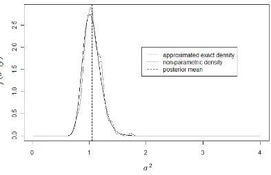
Figure 2.11, 2.12 and 2.13 show the approximated exact posterior densities, compared to the non-parametric densities estimated from the simulated values. In these diagrams, the vertical dotted lines represent the posterior means, which were found to be

, and , while the MCMC estimates are

, and . Hence it is apparent that the MCMC

(34)

[image:34.595.125.526.150.398.2]

Figure 2.11: Approximated exact marginal posterior density of

[image:34.595.120.533.470.757.2]

(35)

[image:35.595.135.528.149.403.2]

Figure 2.13: Approximated exact marginal posterior density of

Next, to assess the coverage of the 95% CPDR of , the MH algorithm was performed again and again to obtain thousand 95% CPDR‟s of , and the number of the 95% CPDR which contains the true value of was determined. Such assessment is computationally intensive (the process took 1 hour and 48 minutes, using the same processor as mentioned above). The R code of the assessment is shown in Appendix B-7. The proportion of the CPDR‟s containing the true value is found to be , with 95% CI of . It appears that the 95% CPDR of is reasonable. Similar can be performed for and , the respective proportions for and were found to be

and , with 95% CI of and .

(36)

a thousand of these PI‟s were obtained to estimate the

proportion containing the true value of . Note that the true value of is known in advance through the same generating process as in Subsection 2.5.1, but never used in the MH algorithm. It is found that the proportion of the 95% PI‟s containing is , with 95% CI . This interval does not contain , suggesting that the prediction interval is not appropriate. However, it is important to understand that the proportion is just an estimate based on a thousand runs of the MH algorithm, and that the PI itself is an estimate from the MCMC methods; due to the random nature of the simulation process, such estimates are rarely exactly the same as the true values.

2.5.8 WinBUGS implementation of the MCMC methods

This subsection repeats the above analysis with WinBUGS, for which Gibbs sampler will be used. Note that the minimum burn-in allowed in WinBUGS is , hence, to obtain an effective sample size of , simulations were performed. The priors are also modified slightly as WinBUGS does not allow the priors to be improper; they are now

(37)

shown under the labels „2.5%‟ and „97.5%‟. The „MC error‟ in Table 2.4 corresponds to the batch means approach:

MC error batch means standard deviation

Table 2.4: Estimated posterior quantities (WinBUGS output)

node mean sd MC error 2.5% median 97.5%

alpha 0.07605 0.1035 0.003158 -0.1255 0.07713 0.2849 beta 0.5626 0.08371 0.003017 0.3966 0.5616 0.7299 eta 0.1724 0.2491 0.007584 -0.3379 0.1784 0.646 sigma2 1.055 0.1581 0.005542 0.8016 1.037 1.408 tau2 2.517 0.7089 0.0239 1.595 2.382 4.286

Note that with the exception of parameter , the estimated posterior means are very close to the estimates obtained via MH algorithm. With reference to the true posterior mean of from Subsection 2.5.7, WinBUGS performs better in estimating the posterior mean of , owing to the fact that Gibbs sampler is more efficient.

Performing predictive inference with WinBUGS is much simpler than writing the code in R, in which one only need to specify the formulae and/or the distributions of the desired quantities. The following shows the next ten forecasted values of , together with their 95% PI‟s shown under the labels „2.5%‟ and „97.5%‟.

Table 2.5: Predictive inference of future values (WinBUGS output)

(38)

Hypothesis testing can be slightly harder to implement in WinBUGS, as the posterior predictive p-value is determined using the „step‟ function; refer to the WinBUGS user manual by Spiegelhalter et al. (2003) for more details. Carrying out the same hypothesis test as Subsection 2.5.6, where the null hypothesis is , the ppp-value is again found to be zero. The WinBUGS code for the alternative time series model for hypothesis testing is shown in Appendix C-2.

(39)

C

l

a

i

m

R

u

n

-

o

f

T

r

i

a

n

g

l

e

s

a

n

d

D

a

t

a

3.1 Claim run-off triangles

A claim run-off triangle is a presentation used by actuaries, showing the claim liabilities which are long-tailed in nature, meaning that the claims usually take months or years to be fully realised. In a claim run-off triangle, the rows correspond to the years in which accidents or claim events occurred (accident years), while the columns show the years elapsed in which the claims are paid out (development years). An example of a claim run-off triangle is presented in Table 3.1 in the next section.

Note that a claim run-off triangle contains empty cells, which are associated to claim liabilities that are not yet realised. The area in which the cells are empty is generally referred as the lower triangle. The total (sum) of the values in the lower triangle equals the required reserve.

3.2 The AFG data

(40)

Since it is unclear on the exact timing of these claims, the calendar year for which the first claim (corresponding to entry , which has a value of ) occurred is defined to be year . Consequently, the calendar year associated with each entry

is , for example, the calendar year associates with entry is year .

Also note that the value of the in the run-off triangle is in unit of , for instance, the cumulative incurred claim amounts for entry is .

Table 3.1: AFG data - cumulative incurred claim amounts

Accident year i

Development Year j

0 1 2 3 4 5 6 7 8 9

1 5,012 8,269 10,907 11,805 13,539 16,181 18,009 18,608 18,662 18,834 2 106 4,285 5,396 10,666 13,782 15,599 15,496 16,169 16,704 3 3,410 8,992 13,873 16,141 18,735 22,214 22,863 23,466

4 5,655 11,555 15,766 21,266 23,425 26,083 27,067

5 1,092 9,565 15,836 22,169 25,955 26,180

6 1,513 6,445 11,702 12,935 15,852

7 557 4,020 10,946 12,314

8 1,351 6,947 13,112

9 3,133 5,395

10 2,063

The exact claim amounts can be obtained from the difference between successive cumulative claim amounts . These are presented in Table 3.2. To illustrate, the exact

(41)

entry is negative; such a negative claim amount could be the result of salvage recoveries, rejection of claims or cancellation due to initial overestimation of the claim liabilities.

Table 3.2: AFG data - exact incurred claim amounts

0 1 2 3 4 5 6 7 8 9

1 5,012 3,257 2,638 898 1,734 2,642 1,828 599 54 172

2 106 4,179 1,111 5,270 3,116 1,817 -103 673 535

3 3,410 5,582 4,881 2,268 2,594 3,479 649 603

4 5,655 5,900 4,211 5,500 2,159 2,658 984

5 1,092 8,473 6,271 6,333 3,786 225

6 1,513 4,932 5,257 1,233 2,917

7 557 3,463 6,926 1,368

8 1,351 5,596 6,165

9 3,133 2,262

(42)

B

a

y

e

s

i

a

n

M

o

d

e

l

i

n

g

o

f

t

h

e

A

F

G

D

a

t

a

4.1 Reserving methods

As discussed in Chapter 1, deterministic approaches to reserving include the traditional chain-ladder (CL) method and the Bornhuetter-Ferguson method. However, these approaches only provide point estimates of the required reserve. Stochastic reserving methods were considered by Scollnik (2004), England & Verrall (2002) and several others.

The required reserve is equal to the value of outstanding claims liabilities, in which the liabilities may or may not discounted to present value. In the thesis, the outstanding claims liabilities are not discounted to present value, this is to facilitate comparison between different reserving methods. Note that the actual reserve held in practice might not be the same as the required reserve; it is conservative to ensure that the actual reserve is at least as great as the required reserve. For convenience the term „reserve‟ will be used to mean the required reserve instead of actual reserve in this thesis.

More precisely, in a claim run-off triangle showing exact claim amounts (such as the one in Table 3.2), the reserve is equal to the sum of the claim liabilities associated with the lower triangle, which need to be estimated. Equivalently, for a cumulative claim run-off triangle (such as in Table 3.1), the reserve has the following formula:

(43)

It is important to note that the accident year starts from while the development year starts from .

This thesis develops Bayesian models based on classical reserving models first proposed by Hertig (1985) and later extended by de Jong (2004). These Bayesian models, together with their classical counterparts, are discussed in the following section.

4.2 Bayesian models

Consider a run-off triangle with entries which represents the cumulative claim liabilities for accident years and development years . Define the development factors

for as the continuous growth rates in cumulative claim liabilities of accident

years in development year , and formulate this quantity as the log-link ratio. Also define as the natural logarithm of the initial claim liabilities of accident year . Thus:

The variable denotes number of years for which data are available; note that the claim run-off triangle considered in the thesis (AFG data) has equal numbers of rows and columns.

(44)

factors, for which are not the growth rates of the cumulative claims. Also note that the development factors tend to decrease across development years.

Table 4.1: AFG data - development factors

0 1 2 3 4 5 6 7 8 9

1 8.520 0.501 0.277 0.079 0.137 0.178 0.107 0.033 0.003 0.009 2 4.663 3.699 0.231 0.681 0.256 0.124 -0.007 0.043 0.033

3 8.134 0.970 0.434 0.151 0.149 0.170 0.029 0.026

4 8.640 0.715 0.311 0.299 0.097 0.107 0.037

5 6.996 2.170 0.504 0.336 0.158 0.009

6 7.322 1.449 0.596 0.100 0.203

7 6.323 1.976 1.002 0.118

8 7.209 1.637 0.635

9 8.050 0.543

10 7.632

Hertig (1985) made an assumption that the development factors are uncorrelated and can be written in the following form:

(1)

Hence, each has a normal distribution with mean and variance ; that is,

(45)

method of moments, as, for example, in de Jong (2004). In contrast, the Bayesian approach treats the parameters and as random variables, with a joint prior distribution. Often these parameters are taken as a priori independent, uninformative and improper, as follows:

As mentioned before, care must be taken when using improper priors since this might lead to posterior distributions being improper, giving nonsensical inference. Note that actuaries typically have some prior knowledge regarding the parameters, which may be available through past experience, or simply based on their actuarial judgement; the prior distributions can then be modified accordingly.

Hertig‟s model assumes that the growth rates across accident years have the same distribution on each development year . However, de Jong found that the development factors are correlated and suggested adding correlation terms to Hertig‟s model. The following are three different modifications to Hertig‟s model (1) suggested by de Jong.

i. (2)

(46)

ii. Under this accident correlation model, correlation of the development factors

across accident years is modelled by the parameters and .

iii.

This calendar correlation model introduces the parameters and to model the correlation of across calendar years.

(47)

A

n

a

l

y

s

i

s

a

n

d

R

e

s

u

l

t

s

5.1 Hertig‟s model

Hertig‟s model, introduced in Section 4.2, will be used in this chapter to model the AFG data. Ideally, the prior distributions of this model‟s parameters are uninformative and improper, as follows:

However, as the modelling will be done in WinBUGS, which does not allow priors to be improper, the following vague prior distributions are chosen in an attempt to give the best representation of the uninformative and improper priors:

Note that choosing a prior distribution which is more diffuse for and , such as

, leads to an error message in WinBUGS. This is because the

(48)

The WinBUGS code for this model is presented in Appendix C-3. With the starting points chosen to be , and , simulated values of each parameter were created (in 6 seconds, with the same processor described above) via the Gibbs sampler. By burning-in the first simulated values, estimates of the posterior means were obtained from the remaining simulations; the WinBUGS output is displayed in Table 5.1. Classical estimates by de Jong are included for comparison. Note that in Table 5.1, each h[j] corresponds to parameter , while each mu[j]

corresponds to parameter and sigma2 corresponds to parameter .

Table 5.1: Posterior estimates of , and (Hertig‟s model)

node mean sd MC error 2.5% median 97.5% de Jong’s

h[2] 0.9654 0.3503 0.008836 0.4693 0.9088 1.793 0.8571 h[3] 0.2448 0.09868 0.002577 0.1122 0.2254 0.4892 0.2143 h[4] 0.2142 0.09374 0.002222 0.09399 0.195 0.4497 0.1786 h[5] 0.05783 0.02786 6.26E-4 0.02417 0.05152 0.1309 0.0446 h[6] 0.07323 0.04005 9.275E-4 0.02874 0.06386 0.1738 0.0536 h[7] 0.05735 0.04021 8.36E-4 0.01953 0.04666 0.1623 0.0357 h[8] 0.01322 0.01739 5.151E-4 0.003171 0.008864 0.04989 0.0089 h[9] 0.09772 0.3435 0.01146 0.006977 0.02854 0.6174 0.0089 h[10] 0.8656 3.246 0.1542 3.468E-10 0.001739 9.444 0.00

mu[1] 7.346 0.4009 0.003863 6.549 7.345 8.147 7.35 mu[2] 1.518 0.3938 0.004067 0.7263 1.518 2.311 1.52 mu[3] 0.4981 0.1079 0.001066 0.2839 0.4984 0.7141 0.50 mu[4] 0.2515 0.1006 0.00104 0.04582 0.2527 0.4482 0.25 mu[5] 0.1666 0.0297 3.031E-4 0.1069 0.1667 0.226 0.17 mu[6] 0.1182 0.04235 4.402E-4 0.03564 0.1178 0.2026 0.12 mu[7] 0.0409 0.04056 4.143E-4 -0.03797 0.04104 0.118 0.04 mu[8] 0.03362 0.01372 1.166E-4 0.01118 0.03389 0.05449 0.03 mu[9] 0.01951 0.2885 0.001898 -0.1811 0.01824 0.24 0.02 mu[10] -0.01621 3.873 0.03726 -3.992 0.009174 4.147 0.01 sigma2 1.612 0.8962 0.03325 0.626 1.387 3.965 1.2544

(49)

become smaller with time after the accident year. The estimates of follow the same pattern, with the exception of , and .

Thirdly, note that the estimates of and are very large, with extremely large standard deviations and wide 95% CPDR‟s compared to the other (see the bolded figures in Table 5.1). The reason behind this is that there are only a few data points available to estimate these parameters, as can be seen on the right hand side of the claim run-off triangle. Since uninformative priors are used, lack of data points leads to the posterior distributions being highly disperse. Note that this problem is also present in the estimates of and .

Finally, the estimates of are found to be very close to the classical estimates obtained by de Jong. On the other hand, the variability of the development factors, captured by the parameters and , are found to be higher than the classical estimates. However, the classical approach tends to underestimate uncertainty regarding the parameters. This is most apparent for , de Jong took as since there is only one data point corresponding to (in which case the variability cannot be estimated).

(50)

[image:50.595.137.544.197.770.2]

(extremely large values) in Figure 5.3 is the primary reason for the high standard deviation of the estimate (see Table 5.1). The traces of the simulated are similar and give the same inference for . The traces of simulated , and are shown in Appendix D-2 for completeness.

Figure 5.1: Trace of simulated

Figure 5.2: Trace of simulated

Figure 5.3: Trace of simulated mu[2]

iteration

1 5000 10000

-2.0 0.0 2.0 4.0

mu[6]

iteration

1 5000 10000

-0.5 0.0 0.5 1.0

mu[10]

(51)

Predictive inference on the future development factors can be obtained by generating random observations of the future development factors directly. In WinBUGS, this is easily done by specifying the distribution of the future development factors, which is no different from the distribution of the current development factors, as defined in Section 4.2. In addition, the future cumulative claim liabilities and the reserve are readily obtained since they can be expressed as explicit functions of the future development factors. The predictive inference is presented in Table 5.2 in the same format as Table 5.1; again, note that each delta[i,j] corresponds to the development factor .

Most of the predicted development factors are reasonable predictions of the future, except for development years and , where the high variability in predictions is caused by the imprecise posterior estimates of the underlying parameters. For instance, the prediction of (delta[10,10] in Table 5.2) is accompanied by an extremely large standard deviation and a very wide 95% prediction interval . These large standard deviations and prediction intervals are bolded in Table 5.2; they correspond to the estimates where . These predictions do not provide any real information regarding the future claim amounts, because a single data point is insufficient to project future claim payments. For example, the 95% prediction interval for suggests that the cumulative claim liabilities for next year will be between

(52)

[image:52.595.154.502.115.603.2]

Table 5.2: Predictive inference on the future (Hertig‟s model)

delta[2,10] -0.06639 5.792 0.05582 -6.386 0.009174 4.653

delta[3,9] 0.02169 0.4779 0.005613 -0.3242 0.01859 0.4005 delta[3,10] -0.0766 5.8 0.05948 -5.966 0.009174 5.193

delta[4,8] 0.03373 0.02775 2.721E-4 -0.01056 0.03376 0.07774 delta[4,9] 0.0194 0.5035 0.003882 -0.3461 0.01726 0.3832 delta[4,10] -0.04602 5.278 0.05102 -5.723 0.009174 5.258

delta[5,7] 0.04168 0.08435 7.927E-4 -0.1306 0.04108 0.2113 delta[5,8] 0.03362 0.02701 2.492E-4 -0.01203 0.03359 0.07488 delta[5,9] 0.02299 0.4981 0.004636 -0.3235 0.01821 0.4023 delta[5,10] 0.01581 5.405 0.03206 -5.733 0.009174 5.721

delta[6,6] 0.1181 0.1037 0.00111 -0.08619 0.1187 0.3224 delta[6,7] 0.0414 0.0922 9.204E-4 -0.1322 0.04117 0.225 delta[6,8] 0.03348 0.02793 2.81E-4 -0.01262 0.03348 0.07792 delta[6,9] 0.0274 0.6109 0.004985 -0.3262 0.01809 0.4015 delta[6,10] -0.02916 6.729 0.05375 -5.362 0.009174 5.28

delta[7,5] 0.1662 0.07821 7.713E-4 0.006882 0.1655 0.3289 delta[7,6] 0.1186 0.1057 0.001188 -0.09621 0.1186 0.3297 delta[7,7] 0.04133 0.0885 8.649E-4 -0.1293 0.04182 0.2084 delta[7,8] 0.03307 0.03147 3.291E-4 -0.01337 0.03376 0.07435 delta[7,9] 0.02044 0.5108 0.005545 -0.3044 0.01844 0.3958 delta[7,10] -0.01812 5.94 0.05174 -6.015 0.009174 6.19

delta[8,4] 0.2552 0.2903 0.003011 -0.3112 0.2522 0.8456 delta[8,5] 0.1674 0.07901 7.884E-4 0.01359 0.1667 0.3249 delta[8,6] 0.1174 0.105 9.475E-4 -0.08331 0.1173 0.3176 delta[8,7] 0.04268 0.09128 9.016E-4 -0.1322 0.04109 0.224 delta[8,8] 0.03385 0.02704 2.47E-4 -0.009508 0.03392 0.07699 delta[8,9] 0.01833 0.5527 0.004303 -0.3269 0.01807 0.4282 delta[8,10] -0.01818 5.352 0.04204 -6.319 0.009174 5.553

delta[9,3] 0.5033 0.3174 0.002829 -0.1371 0.5049 1.135 delta[9,4] 0.2473 0.2803 0.003139 -0.3194 0.2479 0.7994 delta[9,5] 0.166 0.08086 8.958E-4 -0.002365 0.1663 0.3278 delta[9,6] 0.1175 0.1075 0.001102 -0.09249 0.1169 0.3274 delta[9,7] 0.0402 0.09023 9.666E-4 -0.1353 0.03959 0.2169 delta[9,8] 0.03385 0.03023 2.84E-4 -0.01223 0.03376 0.0774 delta[9,9] 0.01652 0.4597 0.005298 -0.3345 0.01874 0.3518 delta[9,10] -0.002851 5.936 0.07171 -5.806 0.009174 5.566

delta[10,2] 1.506 1.225 0.01138 -0.977 1.508 3.946 delta[10,3] 0.4966 0.3173 0.003139 -0.1283 0.4977 1.132 delta[10,4] 0.2549 0.289 0.002871 -0.3159 0.256 0.8419 delta[10,5] 0.1672 0.07973 8.097E-4 0.009221 0.1675 0.3259 delta[10,6] 0.1174 0.1036 0.001107 -0.09371 0.1187 0.3224 delta[10,7] 0.0425 0.08824 8.206E-4 -0.1273 0.04155 0.2132 delta[10,8] 0.0334 0.02738 3.026E-4 -0.01053 0.03362 0.07786 delta[10,9] 0.01795 0.4781 0.00527 -0.3285 0.0181 0.3751 delta[10,10] 0.02923 5.535 0.07309 -5.71 0.009174 5.75

(53)

ways to achieve the predictive inference on the cumulative claim liabilities and the reserve. One method is to reduce the number of effective simulations . The other is to explicitly set an upper bound for the predicted development factors. The predictive inference obtained via the first method with is shown in Appendix D-3 for completeness. A snapshot of the predictive inference is shown in Table 5.3. This inference is not entirely useful, since the predicted reserve is unreasonably large.

Table 5.3: Predictive inference on reserve (Hertig‟s model)

reserve 1.086E+33 4.406E+34 1.067E+33 -75100.0 86260.0 5.208E+11

5.2 A modified Hertig‟s model

As can be seen in the previous section, using a single data point for estimation leads to extremely large standard deviations and hence imprecise estimates. This calls for a modification to Hertig‟s model that rectifies this problem. Since the parameters and decrease with development years , one possible approach is to model the structure of and directly. Assuming and decrease exponentially for , the following parameterisation was used as a „fix‟ to Hertig‟s model:

(54)

The vague prior distributions associated with this modification are as follows:

where forces the simulated values of to be positive (this notation is consistent with WinBUGS syntax).

These priors are not really uninformative; for instance, the parameters , and are deliberately restricted to be positive since it is assumed that the mean of the development factors are positive (a development factor can still be negative under this model). This assumption is supported by the MCMC estimates in Table 5.1.

This modification reduces the number of parameters that need to be estimated from to and assumes that and decrease exponentially with a constant rate. (This assumption could be relaxed by allowing and to decrease with varying rates, but this would increase the required number of parameters.)

As in Section 5.1, Gibbs sampling was used to simulate values of each parameter. The starting points were chosen to be , , ,

(55)

output in Table 5.4. Note that h[j] represents mu[j] represents and sigma2 represents .

Table 5.4: Posterior estimates of , , , and (modified Hertig‟s model)

M 0.5715 0.03239 5.412E-4 0.5051 0.5723 0.6342 N 0.5989 0.03991 8.131E-4 0.5254 0.5972 0.6818 h[2] 0.9303 0.3557 0.009583 0.4297 0.8665 1.83 h[3] 0.2341 0.07353 0.00266 0.1165 0.2249 0.4024 h[4] 0.1388 0.03954 0.001446 0.07263 0.1347 0.2253 h[5] 0.08266 0.02243 7.974E-4 0.0441 0.08074 0.1313 h[6] 0.04945 0.01365 4.485E-4 0.0261 0.0484 0.07896 h[7] 0.02972 0.008864 2.588E-4 0.01517 0.02881 0.05011 h[8] 0.01794 0.006021 1.539E-4 0.008543 0.01715 0.03239 h[9] 0.01088 0.004188 9.444E-5 0.004783 0.01017 0.02096 h[10] 0.006628 0.002942 5.969E-5 0.002635 0.00606 0.01388 mu[1] 7.356 0.4189 0.004546 6.536 7.356 8.191 mu[2] 1.521 0.3949 0.003977 0.7353 1.518 2.319 mu[3] 0.4954 0.07502 0.001277 0.355 0.4927 0.6517 mu[4] 0.2814 0.03336 4.899E-4 0.2161 0.2813 0.3493 mu[5] 0.1604 0.01719 1.755E-4 0.1259 0.1605 0.1946 mu[6] 0.09167 0.01119 9.605E-5 0.06856 0.09184 0.1135 mu[7] 0.05256 0.008153 8.652E-5 0.03586 0.05257 0.06861 mu[8] 0.03023 0.005968 7.427E-5 0.01827 0.03014 0.04223 mu[9] 0.01744 0.004263 5.811E-5 0.009349 0.01729 0.02636 mu[10] 0.01009 0.002971 4.277E-5 0.00475 0.009922 0.01647 sigma2 1.802 1.082 0.04033 0.664 1.511 4.661

Although the output shows 22 parameter estimates, there are only 8 free parameters since and for are essentially functions of the other parameters, namely and . Note that the problem with extremely large standard deviations was eliminated with the reduction in the number of free parameters; hence overall the estimates are more precise, with smaller standard deviations and narrower 95% CPDR‟s. The traces of the simulated values suggest quick convergence and good mixing. Since these traces are similar to the trace in Figure 5.1, they are not displayed here. These traces are available in Appendix D-4 for completeness.

(56)

liabilities and the reserve . Unlike in the preceding section, obtaining the predictive inference with WinBUGS did not produce any error messages under modified Hertig‟s model. The predictive inference is shown in Table 5.5, where c.pred[i,j] represents

[image:56.595.142.511.236.747.2]

.

Table 5.5: Predictive inference on future and (modified Hertig‟s model)

(57)

At first glance, the predictions seem reasonable and the standard deviations associated with each predicted value do not appear to be very large; however, this is only true for

where . For the cumulative claim liabilities at the bottom row of the claim

run-off triangle (i.e. ), the standard deviations are larger than the associated forecasted liabilities, giving imprecise estimates (see the bolded figures in Table 5.5). Consequently, the estimated reserve is also imprecise.

[image:57.595.135.543.536.665.2]

Note that the forecasted means in the predictive inference are larger than the medians, suggesting that the predictive distributions are positively skewed. However, the means corresponding to the last row of the cumulative claim liabilities and reserve appear to be too large compared to their median, suggesting highly dispersed and extremely skewed distributions. This can be seen in Figure 5.4, which depicts the trace of the simulated values of reserve; the extremely large simulated values, which correspond to large spikes in the trace, cause the mean to be much larger than the median. In this case, perhaps the median is a more appropriate choice for predictive purposes.

Figure 5.4: Trace for simulated values of reserve (modified Hertig‟s model) reserve

iteration

1 5000 10000

(58)

The large standard deviations corresponding to the bottom row of the cumulative claim liabilities is most likely to be caused by the imprecise forecast of (c.pred[10,2] in Table 5.5) initially, and this causes the following cumulative claim liabilities to be highly variable, ultimately the estimated reserve as well. It is possible that the model is lacking something in explaining the development factors when , such as the correlation between the development factors. In fact, ignoring the correlation between

and can lead to sizable forecast errors (de Jong, 2004). Correlation between the

development factors will be implemented in the following section.

5.3 Development correlation model

In this section, the development correlation model (see Equation 2 in Section 4.2) is further discussed. Note that this model assumes first order correlation between each consecutive pair of the development factors, in the sense that each is correlated with

for ; this is captured by the correlation parameters .

The same modification from Section 5.2 will be applied to this model (i.e. applying structural constraints to and for ), to avoid large standard deviations that accompany the MCMC estimates (for and when ). The introduction of the correlation terms will increase the number of free parameters by , which is undesirable given the number of data points. For purposes of parsimony, only the correlation between and will be considered, meaning that only one extra parameter will

(59)

The resulting development correlation model may be summarised as follows:

The prior distributions in this model are exactly the same as those in Section 5.2, with the addition of the prior distribution for , as follows:

Note that there are only 9 free parameters in this model. The WinBUGS code of this model is in Appendix C-5. Again, Gibbs sampling was used to simulate values of each parameter, the starting points were chosen to be

and and values were burnt-in.

The posterior estimates are shown below in Table 5.6. Note that the estimate

of is also presented in Table 5.6. As above, h[j]

represents mu[j] represents and sigma2 represents . Also, theta and rho represent and , respectively.

(60)

[image:60.595.152.499.114.380.2]

Table 5.6: Posterior estimates (development correlation model)

M 0.5711 0.03266 5.617E-4 0.5053 0.5718 0.6351 N 0.5986 0.04001 9.132E-4 0.5266 0.5965 0.6829 h[2] 0.2221 0.08752 0.004816 0.09138 0.21 0.4286 h[3] 0.2238 0.075 0.003573 0.1025 0.2147 0.3959 h[4] 0.1325 0.04036 0.002011 0.06373 0.1292 0.2226 h[5] 0.07883 0.02281 0.001146 0.03887 0.07742 0.128 h[6] 0.04711 0.01375 6.633E-4 0.02317 0.04623 0.07715 h[7] 0.02828 0.008831 3.906E-4 0.01361 0.02742 0.04804 h[8] 0.01706 0.005944 2.344E-4 0.007901 0.01626 0.03096 h[9] 0.01034 0.00411 1.435E-4 0.00446 0.009662 0.02039 h[10] 0.006295 0.002878 8.963E-5 0.002477 0.005728 0.01349 mu[1] 7.38 0.4209 0.01947 6.547 7.382 8.21 mu[2] 1.467 0.3476 0.01601 0.7851 1.463 2.147 mu[3] 0.4967 0.07618 0.001229 0.3518 0.4949 0.6543 mu[4] 0.2819 0.03399 4.692E-4 0.2153 0.2815 0.35 mu[5] 0.1606 0.01754 1.775E-4 0.1259 0.1607 0.1951 mu[6] 0.09172 0.01138 1.087E-4 0.06868 0.09181 0.1135 mu[7] 0.05256 0.008263 9.531E-5 0.03594 0.05265 0.06871 mu[8] 0.03021 0.006035 7.938E-5 0.01847 0.03017 0.0425 mu[9] 0.01742 0.004305 6.115E-5 0.009435 0.01728 0.02645 mu[10] 0.01008 0.002996 4.467E-5 0.004837 0.009887 0.01657

rho -0.9576 0.03492 0.001646 -0.9936 -0.9666 -0.8645

sigma2 2.082 1.597 0.09705 0.7158 1.653 6.188 theta -4.141 1.836 0.1221 -8.785 -3.769 -1.72

(61)

[image:61.595.137.543.94.768.2]

Figure 5.7: Trace of mu[1]

iteration

1 5000 10000

5.0 6.0 7.0 8.0 9.0 10.0

mu[2]

iteration

1 5000 10000

0.0 1.0 2.0 3.0 4.0

theta

iteration

1 5000 10000

(62)

[image:62.595.146.505.186.676.2]

Predictive inference on the individual future cumulative claim liabilities and the total reserve are presented in Table 5.7.

Table 5.7: Predictive inference on and (development correlation model)

(63)

close to one another. More importantly, the future cumulative claim liabilities and the reserve have reasonable standard deviations which are not unduly large (see bolded figures). Although the distributions of the predicted claim liabilities and reserve are still positively skewed in this case, the magnitudes of the estimated means are not very large compared to the estimated median.

[image:63.595.139.542.323.446.2]

As can be seen in Figure 5.8, which portrays the trace of the simulated reserve, there appears to be no highly extreme values.

Figure 5.8: Trace of simulated reserve

Comparing Hertig‟s model modified Hertig‟s model, and the development correlation model, it seems that the development correlation model performs best in modelling the claim run-off triangle (AFG data). In the next chapter, these three models will be assessed formally through hypothesis testing.

reserve

iteration

1 5000 10000