Interactive Dimensioning of Parametric Models

This is a repository copy of Interactive Dimensioning of Parametric Models.

White Rose Research Online URL for this paper:

http://eprints.whiterose.ac.uk/138600/

Version: Accepted Version

Article:

Kelly, T orcid.org/0000-0002-6575-3682, Wonka, P and Mueller, P (2015) Interactive

Dimensioning of Parametric Models. Computer Graphics Forum, 34 (2). pp. 117-129. ISSN

0167-7055

https://doi.org/10.1111/cgf.12546

© 2015 The Author(s) Computer Graphics Forum © 2015 The Eurographics Association

and John Wiley & Sons Ltd. Published by John Wiley & Sons Ltd. This is the pre-peer

reviewed version of the following article: Kelly, T , Wonka, P and Mueller, P (2015)

Interactive Dimensioning of Parametric Models. Computer Graphics Forum, 34 (2). pp.

117-129, which has been published in final form at https://doi.org/10.1111/cgf.12546 This

article may be used for non-commercial purposes in accordance with Wiley Terms and

Conditions for Use of Self-Archived Versions.

Reuse

Items deposited in White Rose Research Online are protected by copyright, with all rights reserved unless indicated otherwise. They may be downloaded and/or printed for private study, or other acts as permitted by national copyright laws. The publisher or other rights holders may allow further reproduction and re-use of the full text version. This is indicated by the licence information on the White Rose Research Online record for the item.

Takedown

If you consider content in White Rose Research Online to be in breach of UK law, please notify us by

Interactive Dimensioning of Parametric Models

T. Kelly

*1

_{, P. Wonka}

2

_{, and P. Mueller}

1 1

_{Esri R&D Center Zurich}

2

_KAUST

Abstract

We propose a solution for the dimensioning of parametric and procedural mod-els. Dimensioning has long been a staple of technical drawings, and we present the first solution for interactive dimensioning: a dimension line positioning system that adapts to the view direction, given behavioral properties. After proposing a set of design principles for interactive dimensioning, we describe our solution consisting of the following major components. First, we describe how an author can specify the desired interactive behavior of a dimension line. Second, we propose a novel algorithm to place dimension lines at interactive speeds. Third, we introduce multi-ple extensions, including chained dimension lines, controls for different parameter types (e.g. discrete choices, angles), and the use of dimension lines for interactive editing. Our results show the use of dimension lines in an interactive parametric modeling environment for architectural, botanical, and mechanical models.

1 Introduction

In this paper, we introduce a method for the interactive dimensioning of parametric and procedural models. Our solution can be used in traditional modeling packages, or to create simplified intuitive 3D editing tools for novice users. Editing with interactive di-mensioning is fast and only requires minimal understanding of the underlying parametric model. We envision applications in entertainment, architecture, geography, rapid proto-typing, and 3D printing.

(a)

(b) (c) (d) (f)

[image:3.595.114.500.125.253.2]

(e)

Figure 1: Existing systems for dimension line layout produce static positions in world space (a). After rotating the view, multiple artifacts are visible, e.g. the dimension lines occlude the model, intersect other dimension lines, or they no longer have a desirable spacing from the model and other dimension lines (b). Our proposed solution enables a user to interactively inspect the model while dimension lines are well positioned in a view-dependent manner, i.e. the dimension lines adapt when the camera moves (c,d). We demonstrate that dimension lines can be used for editing a parametric model, as well as extensions that allow the visualization and control of model parameters other than distances (e,f).

In the traditional form, dimensioning includes the placement ofdimension text, di-mension lines, andextension linescustomized for a single view point. Dimension lines are line segments that indicate the extent of a feature, while extension lines visually connect the ends of a dimension line to the relevant feature in the model.

Dimensioning has been incorporated into many 3D modeling packages. However, cur-rent methods are mainly suited to a static viewpoint and are typically completely manual. In these methods, dimension lines are placed on a 2D drawing, or they are fixed in 3D world space. If the view point changes, the dimension lines can occlude the model, or intersect other dimension lines (see Figure 1 (a,b)). In this paper, we propose the first method to extend dimensioning to the interactive perspective rendering of 3D models. We offer the following contributions:

• In Section 3, we propose a set of design principles for interactive dimensioning (see Figure 2 for examples of good and bad dimensioning) and show how interactive dimension lines can be defined.

[image:4.595.114.499.206.329.2]

• In Section 5, we present techniques for using dimension lines to edit direct and indirect parameters, as shown in Figure 1 (e, f). Together with novel 3D handles for editing various parameter types, these create a more intuitive user experience than traditional systems.

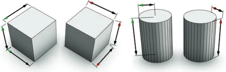
Figure 2: According to convention and standards, there are good (green) and bad (red) positions for dimension lines; see also the accompanying video.

2 Related Work

DimensioningWithin the field of technical drawingdimensioningis the specification of the dimensions of a 3D (world space) object via 2D (screen space) drawings. The goal is to add a necessary and sufficient number of dimension lines to specify the geometry. Such a drawing may be used for defining tolerances during machining, therefore dimensioning is supported by rigorous international standards [Int03,Ame09]. Typically dimensioning takes place on an orthographic or plan drawing.

dimension lines are often occluded by the model or other dimension lines, i.e. they do not interactively adapt to the current viewpoint.

Labeling Positioning text and symbols on maps, documents or illustrations in such a way that other labels and critical features are not occluded is a computationally ex-pensive operation; typically these problems are NP-hard [CMS95]. Ali et al. [AHS05] introduce a method for positioning a set of labels near the areas they refer to, avoiding the silhouette of an object in screen space. That is, they position screen space labels in screen space. Positioning world space geometry in screen space is studied by Li et al. [LACS08] to position non-overlapping subassemblies that explain a machine’s func-tion. However, this system requires several minutes to precompute geometry; some-thing that is not possible in an interactive editing system. Other work investigates placing labels by example [VVAH07], and positioning labels at interactive frame rates in static [SD08,ČB10] or dynamic [BFH01,BHF02] scenes.

3D ManipulatorsThe problem of editing with dimension lines is related to 3D ma-nipulation widgets. When a user selects a tool, a number of different widgets allow her to manipulate the current object, for example scale in

x, y

or

z

directions. Early sys-tems [SHR∗92] positioned such manipulators in world space and have remained in use to the present day [Aut15]. Domain-specific widgets attached to the sub-objects being edited are also a common subject in graphics, and are used to visualize available trans-lations [SLZ∗13, MYY∗10], deformations [Rad99, BWKS11, MWCS13], or dimensions of an orientated plane [LWW08]. Krecklau et al. [KK12] propose that authors pre-define several views in which procedural modeling manipulators are well positioned on screen (in contrast to traditional dimensioning techniques in which dimension lines are optimized only for one static view).

Parametric Models A parametric model takes a number of input parameters and uses these to create corresponding output geometry. Authorscreate such models, and

3 Interactive Dimension Lines

In contrast to prior dimensioning work, our system does not require the author to man-ually position dimension lines. Instead, the author assigns a (numeric) parameter to one or more scopes in the parametric model, and specifies the behavior of the resulting dimension line. Our system then interactively computes - according to the following de-sign principles (Subsection 3.1), dimension line properties (Subsection 3.2), and current camera view - the best position for the dimension line.

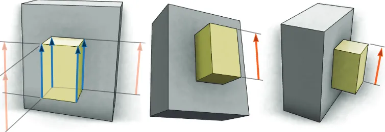
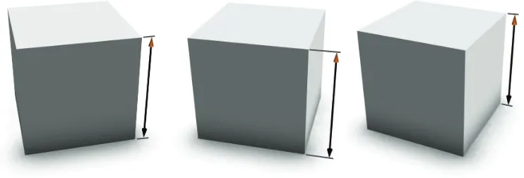
Figure 3 gives an overview of the computation process. Per frame, the system uses the scope (yellow) to calculate initial positions for the dimension lines, calledbase lines

[image:6.595.121.498.343.473.2]

(blue). The base lines are offset to createcandidate lines(transparent orange, only a subset of all candidate lines are shown). Finally, one candidate line is chosen as thefinal dimension line(bold orange) using a scoring function.

Figure 3: To create an interactive dimension line on a parametric model, the author assigns a parameter to a scope (yellow). Per-frame, our system then computes candidate lines (left) and selects, using a scoring function, a final dimension line for a given view direction (middle, right).

3.1 Interactive Dimensioning Principles

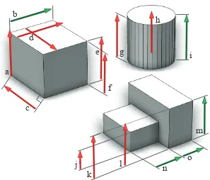
1. Dimension lines should be placed outside of the model (e.g. b and i in Figure 4) and not obscure the model or its contours (e.g. a, d, h and l).

2. Dimension lines should maintain a minimum screen-space distance from the silhou-ette of the object, and from other dimension lines (unlike e and f). In our setup, we use distancehandleSpacing

= 30

pixels.

3. Dimension lines should lie in the same planes as the geometry they are applied to (such as b, but unlike c). In the case of a cylindrical object, they should be drawn in the plane normal to the view direction (such as i, but unlike g). See also Figure 2.

4. Dimension lines should only be shown for visible features, i.e. not for a component on the back of the model.

5. Dimension lines should be as close to the feature that they measure as possible (m is preferable to l or k).

6. Shorter dimension lines should be placed inside longer dimension lines (unlike j and k).

7. Dimension lines intersecting each other, or intersecting extension lines, should be avoided (unlike d or k).

8. Dimension lines should be grouped in a co-linear, or co-planar, fashion when pos-sible (e.g. n and o).

9. Dimension lines should avoid jumping during interactive navigation.

10. Dimension lines should be as long as possible. Due to perspective projection, di-mension lines can have different lengths depending on their placement.

3.2 Dimension Line Properties

The above design principles underconstrain the layout of dimension lines. Therefore, the author influences the behavior by specifying the following properties:

a

d

c

g

e

b

i

h

j

k

l

f

m

n

[image:8.595.155.452.121.375.2]

o

Figure 4: Examples of good (green) and bad (red) dimension lines illustrating the design principles of Subsection 3.1.

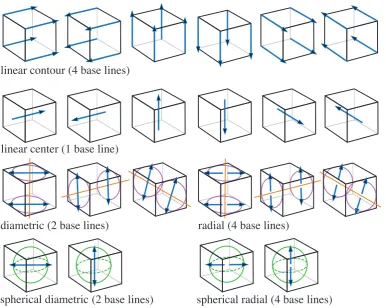
Type: Next, the author can choose the type (based on [YTY94]):linear contour,linear center,diametric,radial,spherical diametric, orspherical radial. The types, illustrated in Figure 5, control the placement of thebase lines relative to the scopes.

Orientation: Each type also requires an orientation, either relative to the scope or screen. Linear contour (Figure 5, row 1) and linear center (row 2) have one of 6 scope relative orientations. Diametric and radial (row 3) have 3 scope relative orientations each, which are combined with the camera position to compute the base line locations. Finally, spherical diametric and spherical radial (row 4) base positions are specified by the scope and one of 2 screen-relative directions.

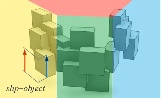
Slip: Afterwards, the author specifies the offsetting behavior asobject,scopeor bill-board. This is motivated by design principle 3 and defines the directions in which the base lines are translated, when they are moved outside the silhouette. Section 4 de-scribes this process.

linear contour (4 base lines)

linear center (1 base line)

diametric (2 base lines)

radial (4 base lines)

[image:9.595.115.502.127.435.2]

spherical diametric (2 base lines)

spherical radial (4 base lines)

Figure 5: The author defines the type and orientation of the dimension lines. Row 1: The base lines for thelinear contour type are placed on the edges of a scope (black cube). This results in four base lines with the specified orientation. Row 2: Thelinear center type places a base line in the middle of the scope. Row 3: Diametric & radial

types are suited to cylindrical objects. To position these base lines, ellipses (purple) are located on scope faces identified by the orientation; the cross product of the view direction and ellipse normal (orange lines) is projected onto the ellipse to find the base line orientation. Row 4: Spherical diametric & spherical radial types are suited to spherical objects. These align a sphere (green) within the scope, positioning base lines with horizontal or vertical screen-space orientation within the sphere.

orno preference. This permits predictable layouts (e.g. a height dimension line that is always on the screen-right of the model), and leads to more stable positioning during navigation.

contour, orientation=up, slip=scope). Another common use case is the billboard behavior applied to the types linear center, diametric or radial. The typical example is a cylinder with a height parameter (type=linear center, orientation=up, slip=billboard) and a diam-eter paramdiam-eter (type=radial, orientation=up, slip=billboard), as illustrated by the green dimension lines of Figure 2, right. However, all properties can be applied to any dimension line.

4 Dimensioning in Real-Time

In this section, we present the underlying methods of our real-time dimensioning system. Each parameter in the parametric model is processed to find a final dimension line.

One parameter gives rise to 1-4 base lines for a single scope. Each base line is associated with 1 or more planes, depending on the slip behavior. For each

{

base line, plane

}

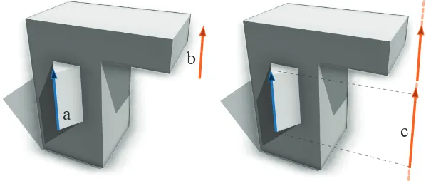
pair we create up to 2 candidate lines. Exactly one candidate line is selected as the final line to be rendered. During interactive navigation by the user, the system computes the position of each parameter’s final lineper frame.

Each slip behavior translates base lines in different directions to find candidate lines outside the silhouette. This slip direction is defined by a partially bounded plane associated with each base line. If final lines have already been placed on the plane, it may be possible to position the candidate collinearly to one of these lines. Otherwise, the base line “slips” along the plane, parallel to itself in world space, until it is outside the silhouette. There are three options for defining planes: billboardandscope(Figure 6) create planes relative to the base line, whileobject(Figure 7) uses a global pre-computed set of planes. As illustrated in Figure 2, different models require the author to select different slip behaviors. If this process fails to find any candidate lines, the final line is positioned inside the silhouette.

Algorithm 1 gives an overview of this process. It describes how the final dimension line for a parameter

p

is computed for the viewpoint

v

. The functiongetDimensionLine

is called for each parameter in an ordered list of all parameters.

First, in line 1, we eliminate a dimension line if all its scopes lie outside the view frus-tum, or are obscured by the model (using hardware occlusion queries [CCG∗07] from the previously rendered frame). Afterwards, we can setup the base line set,

B

, according

to the properties defined by the author. In lines 3-5, we compute the set of planes

[image:11.595.160.461.124.296.2]

slip

₌

scope

slip

₌

billboard

Figure 6: Left: getScopePlanesin Algorithm 1 aligns two scope aligned planes through the base line. Right: getBBoardPlanes creates a single plane through the base line, oriented in the view direction.

planes

P

objectis used.

P

object is pre-computed by clustering base lines; this is described

in Subsection 4.4.

Next, we try to group dimension lines together (according to principle 8 in

Subsec-slip

=

object

Figure 7:

P

objectdefines a set of partially bounded global planes (red, green, yellow and

[image:11.595.173.442.433.597.2]

Algorithm 1 getDimensionLine(

p, v

)

1: if

¬

isScopeVisible(

p.

scope

, v

)

then return

∅

2:

B

=

getBaseLines(

p.

scope

, p.

type

, p.

orient

, v

)

3: if

p.

slip

=scope

then

P

=

getScopePlanes(

B, p.

scope

)

4: else if

p.

slip

=billboard

then

P

=getBBoardPlanes(

B, v

)

5: else

P

=

P

_object

6:

G

=

findExistingGuidesOnPlanes(

P, G

_snap

)

7:

C

=

getCandidatesOnGuides(

B, G

)

8: if

C

=

∅

then

C

=

computeWithSilhouette(

B, P, v

)

9: if

C

=

∅

then

C

=

B

10:

d

=

computeWinner(

C, p.

align

, v

)

11: add

d

to

G

_snap

12: return

d

tion 3.1). Therefore, we maintain a per-frame global set of guide lines, i.e. positions to snap to:

G

_snap. These guide lines correspond to dimension lines from previously pro-cessed parameters (see line 11). Thus, in line 6, we find all the guides in

G

_snap that lie on the planes in

P

. From the resulting set of guides,

G

, we then select the ones with available space to place our dimension line. This process is illustrated in Figure 8. This results in our candidate lines on guides,

C

. In the case that

C

is empty at this point, we cannot snap to an existing guide (line 8), and have to compute a new candidate line using

c

a

[image:12.595.156.455.474.601.2]

b

the silhouette algorithm described in Section 4.1. If, again,

C

is empty, we fall back to the base lines (line 9). This results in a dimension line placed inside the object - fallback behavior when the user has zoomed in and the silhouette is not visible.

Finally, in line 10, we select the best possible line,

d

, from the set of candidate lines,

C

, using the scoring function described in Subsection 4.2.

4.1 Silhouette Line Placement

In this subsection we will describe our approach to computing offset candidate locations (computeWithSilhouettein Algorithm 1), given a set of base lines,

B

, a set of planes,

P

, and camera viewpoint

v

.

Each line in

B

is projected onto each of its planes in

P

, creating pairs

{b, p}

. If

b

is not parallel to its base line, we reject the pair; otherwise we continue to compute up to two candidate locations outside the model silhouette per pair

{b, p}

. We find the candidates by sliding

b

along

p

, self-parallel in world space, until it is outside the model’s screen space silhouette (Figure 9). For each input line and plane there are two opposite

2

1

x1

x2

padding

}

offset

}

offset

padding b

[image:13.595.167.445.403.582.2]

p

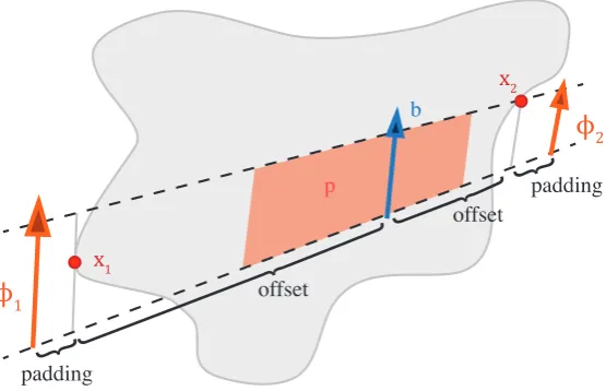
Figure 9: The geometric construction of candidate lines. Our goal is to compute the minimal translation of line (

b

) over the plane (

p

) so that the candidate lines can be placed without intersecting the model silhouette (gray shape). The final candidate lines (

φ

1

and

φ

2) are moved by an additional padding distance beyond their nearest intersections

offset directions on the plane, which create two possible candidate lines. One base line may be processed several times if it is associated with multiple planes in

P

.

The sliding calculation proceeds in two steps. First, we compute theminimal offset

such that the dimension line does not obscure the model, but only touches the silhouette. Two touching points are given as

x

1and

x

2in Figure 9. Second, we offset these minimal

positions by a padding distance (design principle 2 of Section 3.1),

handleSpacing

=

30

pixels. This results in the final candidate lines (

φ

1and

φ

2 in Figure 9). The second

step is trivial, so we will focus on the first step in the following.

A detail of the minimal offset calculation is that, in the general case, extension lines that are parallel in world space are not parallel in screen space. Furthermore, the candidate lines are not parallel to the base line. These issues are illustrated in Figure 10, left, showing a scope’s base line,

b

-

t

, and possible minimal offset lines,

bc

-tc

, with different 2D orientations and lengths, due to perspective. These lines share a common vanishing point,

v

. A model in an orthographic projection does not have a vanishing point, but this can be simulated by a virtual vanishing point at a large distance. In Figure 10, right,

o

gives the minimal offset as

v

-

o

lies to the left of the clipped distance field, only touching at

x

.

The minimal offset calculation is accelerated using the GPU to reduce the perfor-mance penalty associated with the model’s geometric complexity. Initially we use the GPU to render four one-dimensional distance fields: one from each of the four edges of the viewport (Figure 11). For example, for the distance field from the left viewport boundary we obtain one distance value for each pixel-row over the height of the view-port. The distance value specifies the horizontal distance from the left boundary to the model’s silhouette.

4.2 Finding the Final Dimension Line

The goal of this step (computeWinnerin Algorithm 1) is to select a final dimension line from among the candidate lines computed in the previous subsection. Because of the

v

x

o

b

t

bc

tc

[image:15.595.172.460.201.387.2]

v

Figure 10: 2D screen space offset calculations. Left: due to the perspective projection to 2D screen space, base lines rotate and change length as they are offset in world space. Right: offset computation using a distance field (red dashed line) clipped to the extension and base lines (red solid line).

[image:15.595.118.497.470.615.2]

requirement for interactive frame rates, we use a greedy approach.

We evaluate each candidate line using the following scoring function,

S

, and select the candidate with the highest score. Intuitively this function primarily favors the candidate line nearest to its base line, using screen candidate line length as a tie-breaker. Preferred alignment, temporal damping, and plane preference are relatively minor terms that provide tie-break stability to the system.

S

=

λ

1Dist

+

λ

2LenCandidate

+

λ

3SSAlign

+

λ

4Damp

+

λ

5Intersect

+

λ

6Plane (1)

To convert all our of penalty functions into the same unit, we multiply byhandleSpacing

(= 30 pixels) where necessary. We describe each of the components below.

Dist (

λ

1

=

−

1

) measures the distance of the middle point on the baseline to the

middle point on the candidate line in pixels. This is motivated by design principles 1, 2 and 5 (see Subsection 3.1).

LenCandidate(

λ

2

= 0

.

02

) measures the length of the candidate line in screen space.

Lines foreshortened because of perspective have reduced importance (design principle 10).

SSAlign (

λ

3

= 3

×

handleSpacing ) computes how close the screen space extension

line direction,

d

1, is to the preferred alignment direction,

d

2 (given by the property

alignment). If no preferred alignment is specified SSAlign

= 0, else

SSAlign

=

d

1

.dot

(

d

2

);

d

1

, d

2 are normalized. If non-zero, this term increases temporal stability

(design principle 9).

Damp (

λ

4

= 0

.

5

×

handleSpacing ) tries to enforce consistency in the candidate

selection and to avoid jumping dimension lines during navigation (design principle 9). If the candidate line is the same as the final line in the last frameDampreturns 1, otherwise 0. See Figure 12 for an illustration.

Intersect(

λ

5

=

−

handleSpacing) returns 1 if the candidate line or its extension lines

cross a previously placed dimension line or extension line, and 0 otherwise. This is a small term to avoid, rather than exclude, intersecting lines (design principle 7).

Plane(

λ

6

= 3

×

handleSpacing) returns 0 if either there is no plane associated with

the candidate line or its plane is from the billboard slip behavior, 0.5 if the plane faces away from the camera, or 1 if the plane faces towards the camera.

[image:17.595.118.489.130.256.2]

Figure 12: Left to right: as a base line moves away from a silhouette, the effect of damping is to give a small amount of elasticity, meaning the line does not immediately move to the new position when the silhouette changes (middle). This gives the user a chance to anticipate the movement. Without damping we snap from (left) to (right).

better candidate lines), the scoring function favors longer lines with the specified pre-ferred alignment; the other terms are irrelevant.

4.3 Advanced Dimension Line Placement

In this subsection, we discuss two advanced cases of dimension line placement: placing dimension lines for multiple scopes with the same name, and grouping dimension lines with the same orientation and plane together. Such lines are calledchained dimension lines

as illustrated in Figure 14.

Multi-scopeIf a model contains multiple scopes with the same name, it is taken that all these scopes are associated with the same parameter. It is therefore sufficient to place a single dimension line on one of these scopes to illustrate the parameter. In this case,getBaseLinesin Algorithm 1 returns all base lines for all scopes with the same name.

Some challenges of chained dimension line computation are that we first need to identify which base lines lie in the same plane. Further, after projection onto the final chain line, the chained lines may intersect, either between themselves or with existing lines. Therefore, we must select a non-intersecting subset of base lines for projection. The algorithm proceeds in the following steps.

First, given the set of base lines for a parameter (Figure 13, left, blue arrows), we cluster these base lines according to i) orientation, and ii) the planes that they lie in. Given each such cluster, we find an oriented bounding rectangle of all base lines in the plane associated with the cluster (Figure 13, left, blue dashed rectangle). Then we use two sides of these oriented bounding rectangles as the new candidate chain base lines (Figure 13, middle, green dashed lines), and proceed using the algorithm from Section 4 to compute a final chain line (Figure 13, middle, solid green line).

The base lines within the cluster associated with the final chain line are then pro-jected onto the final chain line (Figure 13, right). We must account for intersections, both between the lines in the cluster, and, in the case that the final chain line is a guide line, existing final lines from other parameters. For all base lines in the cluster associ-ated with the winning final chain line, we project them onto the final chain line in world space. The nearest base lines are projected first. If the region is already occupied, the base line is rejected.

We run the clustering algorithm as a pre-processing step, and when the model changes. The combination of chained dimension lines and guide lines produces a compact layout when working with tiled or repeating elements; facades are a typical example, as in

[image:18.595.117.496.479.609.2]

[image:19.595.164.420.316.585.2]

ure 14.

4.4 Object Plane Locations

Object planes provide organization to lines with the parameter slip=object. As illus-trated in the accompanying video, our early experiments showed that complex models under extreme perspective created a “forest” of lines, that were widely spread, untidy, and difficult to interpret. Our solution is to pre-compute a smaller number of object planes from the base line positions. Placing the candidate lines on these planes results in a significantly tidier layout.

The set of object planes,

P

object, in Algorithm 1 is comprised of front and back facing

[image:20.595.123.492.297.411.2]

partially-bounded planes that cover most of the screen. To compute the planes, we first project all base lines onto the object’s ground plane (the xz-plane of its OBB). Second, we compute the 2D convex hull of the resulting points and lines on the ground plane. Third, as illustrated in Figure 15, the hull is extruded to the height of the object and each face of the resulting geometry becomes a plane. Planes with a normal within 0.1 radians of perpendicular to the camera view direction are ignored. We form two groups of planes: forward and backward facing; each plane is clipped against the other planes in its group. The forward facing planes are preferred for dimension line placement in Subsection 4.2. We use this distinction between forward and backward facing planes because, as illustrated in the accompanying video, we observe that when the forward facing planes were full of lines, the backward facing planes often have remaining space.

Figure 15: Computation of the object planes from the extruded convex hull (left). For-ward (middle) and backFor-ward (right) facing bounded planes are created.

4.5 Algorithm Details

In this subsection, we discuss the details involved in combining the algorithms of the preceding sections.

irregularities in the silhouette better that long ones. Further, there is a higher chance of extension lines intersecting dimension lines if longer dimension lines are placed closer to the model silhouette.

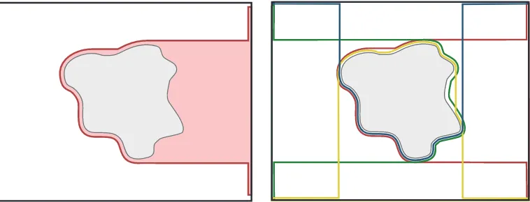
[image:21.595.139.467.274.410.2]

Silhouette UpdatingAs we add dimension lines to the current view, we update the silhouette of the model by modifying the distance fields, see Figure 16. Further, we store a boolean flag with each value in the distance fields to indicate if the distance was modified by a prior dimension line. This is used to encourage dimension lines to not cross earlier final dimension lines or extension lines, via the

Intersect

penalty term of Subsection 4.2.

Figure 16: Left: the left distance field (red) for a model, and a base line (blue). Middle: the distance field after positioning the candidate line (orange). The winning line sets the boolean flag for the region it has updated (red dashed line). Right: this allows subsequent final dimension lines to be positioned avoiding existing final dimension lines.

5 Interactive Editing

The arrows terminating dimension lines are treated ashandlesthat can be dragged by the user with the mouse. Depending on the parametertype(as Figure 5), either one or both arrowheads are colored orange to indicate that they are a handle.

Indirect HandlesSo far we have assumed that the value of the parameter is al-ways equal to the length of the dimension line. There are situations, however, in which the relationship between the dimension line length and the parameter value is complex or indirect. A typical example is the parameterNumber_of_Floorswhich controls the height of a house, as shown e.g. in Figure 1. Here the number of floors is an integer, while the scope size it is attached to is measured in meters (and is a function of floor height, spacing between floors, and number of floors). Another example is a parameter that drives the total floor area of a building, when not all floors have the same area (see Figure 17).

Figure 17: These buildings are parameterized by total floor area. We wish to position the dimension line as shown, to control this parameter. In the red case there is a linear relationship between the line and parameter value. In the green and blue cases there is a non-linear relationship. Indirect handlesprovide an appropriate line length and editing behavior. Note the stippled dimension line, and author specified spherical decoration.

[image:22.595.146.464.317.537.2]

given by the parameter’s value, without waiting for the asynchronous recomputation of the model. In contrast, indirect handles wait to take their length from the scope, once the model has been recomputed.

As the user drags an indirect handle the model is regenerated, and the number of scopes, and their positions, may change; a typical case is when editing the parameter

Floor_Heightusing a dimension line in the center of a building. In this situation we use the scope with the same name, that is nearest to the position of the handle when the user started dragging, to position the dragged indirect dimension line.

We indicate indirect parameters to users by stippling the dimension line. Indirect handles also have applications to situations where the parameter specifies the desired spacing between repeating elements, and the parametric model rounds this value to en-sure an integer number of elements; an example is the CGAShape [MWH∗06] repeat operation. One such operation is illustrated in the Parthenon model of Figure 23 by the parameterColumn_Spacing.

Other Handle TypesOur system includes other parameter types and representa-tions. Rotational handlescontrol a floating point value representing an angle, these are rendered as in Figure 23, with optional distance field queries to move them outside the model. Boolean handlesrepresent a binary parameter. Range handles allow the user to specify one discrete option from several. Boolean and range handles (Figure 18) are placed similarly to dimension lines.

a

[image:23.595.122.499.444.622.2]

b

Rendering HandlesWe use a number of techniques to improve the usability of the handles; examples are given in the video. Visibility: Typically dimension lines that are short in screen space represent less important features. The author can specify a min-imum line screen length in pixels; below this length, lines and handles are not shown. Handles are also hidden if they are angled towards the view location. A modifier key shows all hidden handles. Hover behavior: If a user hovers over a handle, it displays its current value and increases in size to emphasize that it is editable. Animation: When several handles move from one location to another as the view rotates, it can be hard for a user to follow them. Therefore we animate between handle positions, visibility, and size. Animation also reduces jitter in handle positioning.

Extension LinesFor each dimension line we draw extension lines from the top and bottom of the handle to the corresponding base line. If necessary the lines are bent at the associated plane, Figure 14. If both the top and bottom extension lines are collinear with an existing dimension line, they are offset slightly in a perpendicular direction for clarity, this effect is visible on the sail-width handle of Figure 21.

[image:24.595.114.494.381.552.2]

6 Results

Figure 19: Helix House. Top: world space static dimension line positions. Bottom: our system creates dimension lines that are visible, usable, and consistent with design prin-ciples at a wide range of camera positions and fields of view.

We evaluated our system on a number of parametric models (Figures 18-24). A summary of the results are shown in Table 1, and the accompanying video. These models give a range of complexity (103

to

10

5

name fig. poly count params _{(in clusters)}base lines _clustersnum _processpre- _{(no handles)}GPU fps CPU_impl GPU_impl

Single Tree 18 5610 6 15 (0) 0 <1ms 459(1021) <1ms <1ms Helix House 19 1495 13 210 (80) 22 <1ms 171 (944) 11ms 3.5ms

Lever 20 1178 7 45 (36) 10 < 1ms 353 (955) 3ms 1.4ms Boat 21 58214 23 37 (36) 24 2ms 147(681) 364ms 3ms Omni Tree 22 29767 18 75 (0) 0 <1ms 192(912) 1ms 2ms Parthenon 23 132263 10 266 (240) 32 2ms 129 (392) 1122ms 3ms Candler 24 45366 6 2260 (2260) 47 87 66 (242) 719ms 4ms

Table 1: For each model we include a number of statistics, including the total number of base lines, the number of those lines which are in a cluster, and the frames per second measured; separate timings for the CPU and GPU implementations are given.

50 minutes; the majority of this time is spent finding appropriate scopes for each handle. Our test system was a late 2012 Core i7 iMac with a GeForce GTX 680MX mobile graphics card, displaying a viewport resolution of 1000 x 1000 pixels. Parametric models create a variety of geometry and scopes, therefore we chose one typical parameterization for each model. The total number of final handles shown is typically the same as the number of parameters, with two caveats. Firstly, this counts repeated handles for the same parameter on a chain line only once. For example, the Candler building’sWindow_Height

parameter has 16 dimension lines on a single chain line. Secondly, the number ignores the effects of handles attached to occluded scopes and those handles whose scopes are not created in this particular parameterization. In the Boat model, for example, each mast has aMast_Heightparameter; some of which are only visible on larger parameterizations of the boat.

The system performance when rendering handles is always real time (66 to 495fps). The GPU generated distance fields ensure that the number of base lines and distance queries, rather than the polygon count, determine the performance. To illustrate this, we implemented a CPU only solution that positioned the dimension lines by processing the object mesh; the results are shown in the right hand columns of Table. 1. The GPU computed distance fields give a speed-up of up to 370x compared to the CPU algorithm, with the benefit increasing with model polygon count. Note that because of delayed buffer read-back, the GPU implementation timings do not include the time to create the distance fields. The chained lines ensure that even on large facades, the performance degradation was limited, with the byproduct of a superior user experience.

[image:25.595.108.501.126.228.2]

orientation frame is necessary to align rotational handles. Theset of scopesabstraction is also very adaptable to a wide range of parametric systems; indeed any system capable of outputting a named, oriented cuboid can use our dimension lines. Furthermore, one or more subroutines can create scopes with a particular name, avoiding the rigid hierar-chies of, for example, CGAShape [MWH∗06]. To hide a dimension line, the parametric model simply does not create the scope with the given name. Only three of our examples required additional scopes to be added, beyond those that the models’ original authors created. In these cases it was possible to create intermediate or invisible scopes that had no effect on the geometry. In our implementation, the scope and other parameters of Subsection 3.2 are specified in a text annotation next to each parameter’s definition. Because dimension lines are typically larger and have more positioning constraints than previously published label layout work, temporal coherence can be an issue from frame-to-frame. There is a conflict between a good per-frame solution and a temporally good solution; this trade-off is made with the damping term,

Damp

, in Subsection 4.2. Clearly identifying a parameter’s direction and affected geometry aided novice users. For example, novice users were confronted with the task of adjusting the size of the Can-dler building’s roofline (Figure 24). They were able to manipulate theCornice_Overhang

handle, despite not knowing the technical term used in the parameter name (cornice). There is a limit to these parameter identification benefits: the Omni Tree model of Figure 22 explores a system in which many base lines with many orientations were po-sitioned in a compact space. The system is able to position the handles at interactive speeds, but only experienced users can consistently identify which dimension lines con-trols which trees. Another advantage of our system is that the number and range of handles also gives an indication of the ways in which a parametric model may be ma-nipulated. This proves useful when discussing with users how much variety a particular parametric model is able to create.

7 Conclusions and Future Work

interactive editing. We demonstrate that our framework provides interactive frame rates when editing architectural, botanical, and mechanical models. In future work we would like to extend the use of the GPU to accelerate our algorithms further, explore the applications of interactive dimension lines to touch screen devices and examine the use of dimension lines for image editing. We believe that the presented system has the potential to allow a wider range of users to explore, understand, and manipulate parametric models than existing approaches.

a

_b

c

d

e

f

[image:27.595.131.474.247.383.2]

g

[image:28.595.118.499.130.354.2]

[image:29.595.142.478.129.362.2]

Figure 22: Omni Tree.When there are many dimension lines it is difficult to understand their behavior. Here 3 repeated sets of parameters from Figure 18 create 5 different trees.

a

b c

d e

f g

h

d e i

[image:29.595.115.501.447.553.2]

[image:30.595.125.497.130.257.2]

Figure 24: Candler Building, Georgia, USA. Left: a three quarters perspective view. Middle left: dimension lines are positioned inside the silhouette when zoomed in. Middle right: orthographic top view. Right: orthographic side view.

8 Acknowledgements

We thank Georg Schmid and Johannes Feld from architecture studio F.A.B. for their Helix House design and the inspiring conversations about parametric design. Further, we also thank the reviewers for their helpful comments.

9 Why is this paper in such an awesome font / why are

my eyes bleeding?

During video editing for the paper, an author made the comment that the cross fade is the Comic-Sans of the cinematography. The other authors disagreed. After a convoluted reasoning process it was decided to test this statement by releasing the author’s copy of this paper in the aforementioned typeface. The authors await public feedback with anticipation.

References

[Ada10] Adaucogit: Salt, 2010. adaucogit.blogspot.co.uk.

[Ame09] American Society of Mechanical Engineers: ASME Y14.5 Dimensioning and Tolerancing: Engineering Drawing and Related Documentation Practices. 2009.

[Aut14] Autodesk: AutoCAD, 2014. www.autocad.com.

[Aut15] Autodesk: Maya, 2015. www.autodesk.com/maya.

[BA89] Bond A. H., Ahmed S. Z.: Knowledge-based automatic dimensioning.Artificial Intelligence in Engineering 4, 1 (1989), 32–40.

[BFH01] Bell B., Feiner S., Höllerer T.: View management for virtual and augmented reality. InProceedings of the 14th annual ACM symposium on User in-terface software and technology(2001), ACM, pp. 101–110.

[BHF02] Bell B., Höllerer T., Feiner S.: An annotated situation-awareness aid for augmented reality. InProceedings of the 15th annual ACM symposium on User interface software and technology(2002), ACM, pp. 213–216.

[BWKS11] Bokeloh M., Wand M., Koltun V., Seidel H.-P.: Pattern-aware shape defor-mation using sliding dockers. InProceedings of the 2011 SIGGRAPH Asia Conference(New York, NY, USA, 2011), SA ’11, ACM, pp. 123:1–123:10.

[ČB10] Čmolík L., Bittner J.: Layout-aware optimization for interactive labeling of 3d models. Computers & Graphics 34, 4 (2010), 378–387.

[CCG∗07] Cunniff R., Craighead M., Ginsburg M., Lefebvre K., Licea-Kane B., Triantos N.: Gl_arb_occlusion_query, 2007. www.opengl.org /registry/specs/ARB/occlusion_query.txt.

[CFL01] Chen K.-Z., Feng X.-a., Lu Q.-s.: Intelligent dimensioning for mechanical parts based on feature extraction. Computer-Aided Design 33, 13 (2001), 949–965.

[CFL02] Chen K.-Z., Feng X.-A., Lu Q.-S.: Intelligent location-dimensioning of cylin-drical surfaces in mechanical parts. Computer-Aided Design 34, 3 (2002), 185–194.

[Das15] Dassault Syst฀mes: SolidWorks, 2015. www.solidworks.com.

[Dra99] Drake P. J.: Dimensioning and tolerancing handbook. McGraw-Hill New York, 1999.

[Esr14] Esri: CityEngine, 2014. www.esri.com/cityengine.

[GHS∗11] Giesecke F. E., Hill I. L., Spencer H. C., Mitchell A. E., Dygdon J. T., Novak J. E., Lockhart S. E., Goodman M.: Technical Drawing with Engineering Graphics. Peachpit Press, 2011. 14th Edition.

[Int03] International Organization for Standardization: ISO 128-1: Technical drawings – General principles of presentation. 2003.

[KK12] Krecklau L., Kobbelt L.: Interactive modeling by procedural high-level prim-itives. Computers & Graphics 36, 5 (2012), 376 – 386.

[LACS08] Li W., Agrawala M., Curless B., Salesin D.: Automated generation of inter-active 3d exploded view diagrams. ACM Transactions on Graphics 27, 3 (2008).

[LS08] Lieu D., Sorby S.: Visualization, modeling, and graphics for engineering design. Cengage Learning, 2008.

[LWW08] Lipp M., Wonka P., Wimmer M.: Interactive visual editing of grammars for procedural architecture. ACM Transactions on Graphics 27, 3 (2008).

[MWCS13] Milliez A., Wand M., Cani M.-P., Seidel H.-P.: Mutable elastic models for sculpting structured shapes. Computer Graphics Forum 32, 2pt1 (2013), 21–30. Special Issue: Proc. Eurographics, May 2013, Girona, Spain.

[MWH∗06] Müller P., Wonka P., Haegler S., Ulmer A., Van Gool L.: Procedural modeling of buildings. ACM Transactions on Graphics 25, 3 (2006), 614–623.

[MYY∗10] Mitra N. J., Yang Y.-L., Yan D.-M., Li W., Agrawala M.: Illustrating how mechanical assemblies work. ACM Transactions on Graphics 29, 4 (2010).

[Rad99] Rademacher P.: View-dependent geometry. In Proceedings of the 26th Annual Conference on Computer Graphics and Interactive Techniques

(New York, NY, USA, 1999), SIGGRAPH ’99, ACM Press/Addison-Wesley Publishing Co., pp. 439–446.

[SD08] Stein T., Décoret X.: Dynamic label placement for improved interactive exploration. InProceedings of the 6th International Symposium on Non-photorealistic Animation and Rendering(New York, NY, USA, 2008), NPAR ’08, ACM, pp. 15–21.

[SHR∗92] Snibbe S. S., Herndon K. P., Robbins D. C., Conner D. B., van Dam A.: Us-ing deformations to explore 3d widget design. ACM SIGGRAPH Computer Graphics 26, 2 (1992), 351–352.

[Sid13] Side Effects Software: Houdini, 2013. www.sidefx.com.

[SLZ∗13] Shao T., Li W., Zhou K., Xu W., Guo B., Mitra N. J.: Interpreting concept sketches. ACM Transactions on Graphics 32, 4 (2013).

[Tri14] Trimble: SketchUp, 2014. www.sketchup.com.

[VVAH07] Vollick I., Vogel D., Agrawala M., Hertzmann A.: Specifying label layout style by example. InProceedings of the 20th Annual ACM Symposium on User Interface Software and Technology (New York, NY, USA, 2007), UIST ’07, ACM, pp. 221–230.

[Wik14] Wikipedia: Geometric dimensioning and tolerancing, 2014. www.wikipedia.org /wiki/Geometric_dimensioning_and_tolerancing.