Rochester Institute of Technology
RIT Scholar Works
Theses
Thesis/Dissertation Collections
7-1-2011
Investigating low-bitrate, low-complexity H.264
region of interest techniques in error-prone
environments
Timothy Sperr
Follow this and additional works at:
http://scholarworks.rit.edu/theses
This Thesis is brought to you for free and open access by the Thesis/Dissertation Collections at RIT Scholar Works. It has been accepted for inclusion in Theses by an authorized administrator of RIT Scholar Works. For more information, please [email protected].
Recommended Citation
Investigating Low-Bitrate, Low-Complexity H.264 Region of Interest
Techniques in Error-Prone Environments
by
Timothy S. Sperr
A Thesis Submitted in Partial Fulfillment of the Requirements for the Degree of Master of Science in Computer Engineering
Supervised by
Dr. Marcin Łukowiak
Department of Computer Engineering Kate Gleason College of Engineering
Rochester Institute of Technology Rochester, NY
July, 2011
Approved By:
_________________________________________________________________________________________________________
Dr. Marcin Łukowiak
Primary Advisor – R.I.T. Dept. of Computer Engineering
_________________________________________________________________________________________________________
Dr. Andres Kwasinski
Secondary Advisor – R.I.T. Dept. of Computer Engineering
_________________________________________________________________________________________________________
Dr. Michael Kurdziel
Committee Member – Harris Corporation
_________________________________________________________________________________________________________
Duncan Harris
i
Acknowledgements
I would like to thank my advisor Dr. Marcin Łukowiak for making this endeavor possible, as well as for his support and patience throughout this thesis and its related research efforts. I would also like to thank Dr. Andres Kwasinski, for heading up several research projects that led up to this thesis. To the other members of the committee, Dr. Michael Kurdziel and Duncan Harris, thanks also go out for their support and interest. Special thanks go out to the Harris Corporation for providing the impetus for this investigation.
ii
Abstract
The H.264/AVC video coding standard leverages advanced compression methods to provide a significant increase in performance over previous CODECs in terms of picture quality, bitrate, and flexibility. The specification itself provides several profiles and levels that allow customization through the use of various advanced features. In addition to these features, several new video coding techniques have been developed since the standard’s inception. One such technique known as Region of Interest (RoI) coding has been in existence since before H.264’s formalization, and several means of implementing RoI coding in H.264 have been proposed.
Region of Interest coding operates under the assumption that one or more regions of a sequence have higher priority than the rest of the video. One goal of RoI coding is to provide a decrease in bitrate without significant loss of perceptual quality, and this is particularly applicable to low complexity environments, if the proper implementation is used. Furthermore, RoI coding may allow for enhanced error resilience in the selected regions if desired, making RoI suitable for both low-bitrate and error-prone scenarios.
iii
Table of Contents
Acknowledgements ... i
Abstract ... ii
Table of Contents ... iii
List of Figures ... v
List of Tables ... vii
Glossary of Terms ... viii
Chapter 1
Introduction ... 1
1.1.
Motivation for Low-Bitrate, Low-Complexity Region of Interest Coding ... 1
1.2.
H.264 Advanced Video Coding ... 1
1.3.
H.264 Profiles and Levels ... 4
1.4.
Region of Interest Coding in H.264 ... 5
1.5.
H.264 JM Reference Software ... 7
1.6.
Project Goals & Assumptions ... 7
Chapter 2
Theory ... 9
2.1.
H.264 Rate Control Model ... 9
2.2.
H.264 Flexible Macroblock Ordering Techniques ... 13
2.3.
Video Distortion Modeling ... 15
2.4.
Selected RoI Coding Techniques ... 17
2.4.1
Method 1 – Maximum Bit Transfer ... 17
2.4.2
Method 2 – Content-Based Bit Allocation ... 18
2.4.3
Method 3 – Multiple-Priority RoI Coding ... 20
2.4.4
Method 4 – Error Resilience via Nonlinear Transform ... 22
2.4.5
Method 5 – RoI Coding with Flexible Macroblock Ordering ... 25
2.4.6
Method 6 – Explicit Spiral Interleaving ... 27
Chapter 3
Design ... 29
3.1.
Baseline Software Code Modifications ... 29
3.1.1
High Profile Feature Removal ... 29
3.1.2
Main Profile Feature Removal ... 31
iv
3.1.4
Removal of Additional Features ... 32
3.1.5
Baseline Modification Results ... 34
3.1.6
Remaining Features ... 35
3.2.
Error Modeling Code Modifications ... 36
3.3.
Moving RoI Modifications ... 42
3.4.
Video Distortion Software ... 43
3.5.
RoI Coding Technique Modifications ... 43
Chapter 4
Testing ... 47
4.1.
Testing Environment ... 47
4.1.1
Hardware/Software Setup ... 47
4.1.2
Scripting Environment ... 47
4.2.
Experimental Parameters ... 49
Chapter 5
Results & Analysis ... 55
5.1.
Accuracy of Error Model ... 55
5.2.
Results for Rate Control RoI Methods ... 57
5.2.1
Control Group ... 57
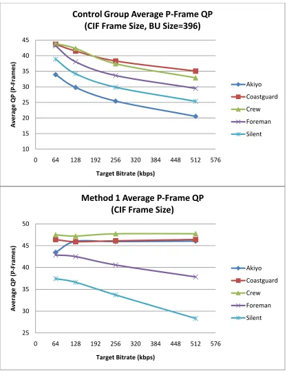
5.2.2
Method 1 ... 63
5.2.3
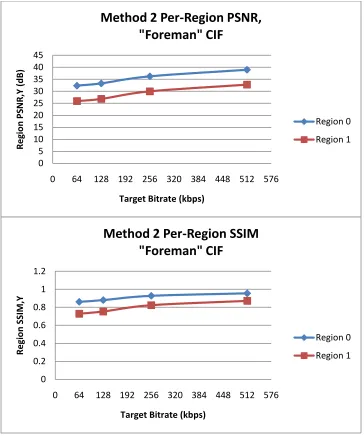
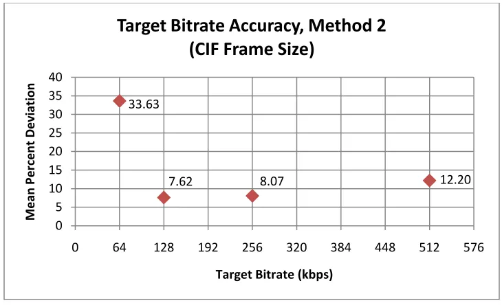
Method 2 ... 69
5.2.4
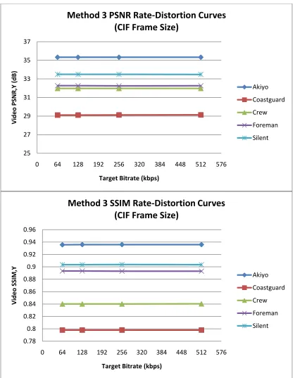
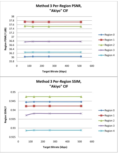
Method 3 ... 73
5.3.
Results for Error Resilience RoI Methods ... 77
5.3.1
Control Group ... 77
5.3.2
Method 4 ... 84
5.3.3
Method 5 ... 93
5.3.4
Method 6 ... 97
Chapter 6
Conclusions ... 102
Future Work ... 104
References ... 106
v
List of Figures
Figure 1.1 H.264 CODEC Block Diagram ... 2
Figure 1.2 Features of the H.264 Baseline, Extended, Main, and High Profiles [3] ... 5
Figure 1.3 Typical Region of Interest Incorporating Subject's Face ... 6
Figure 2.1 Typical Rate-Quantization Curve ... 10
Figure 2.2 Rate-Quantization Curve with Varying Source Complexity ... 10
Figure 2.3 Layers of Rate Control in H.264 ... 12
Figure 2.4 Example Foreground/Background FMO Mapping [3] ... 15
Figure 2.5 Example of Nonlinear Transform with Background Loss ... 23
Figure 2.6 Advanced FMO Mapping Proposed for Method 3 ... 26
Figure 2.7 Explicit Spiral Interleave (ESI) FMO Mapping [13] ... 27
Figure 3.1 CIF Coastguard Video with Coefficient Errors ... 40
Figure 3.2 CIF Foreman Video with Motion Vector Errors ... 41
Figure 3.3 CIF Foreman Video (Frame 1) with Method 4 Transform Applied ... 46
Figure 3.4 CIF Foreman Video (Frame 1) with Method 4 Forward and Inverse Transforms Applied ... 46
Figure 4.1 Method 3 Region Mapping Example ... 53
Figure 5.1 Coefficient Error Model Accuracy Histograms ... 55
Figure 5.2 Motion Vector Error Model Accuracy Histograms ... 56
Figure 5.3 PSNR Rate-Distortion Curves for Control Group ... 58
Figure 5.4 SSIM Rate-Distortion Curves for Control Group ... 59
Figure 5.5 Control Group Per-Region PSNR ... 60
Figure 5.6 Control Group Per-Region SSIM ... 61
Figure 5.7 Control Group Target Bitrate Accuracy ... 62
Figure 5.8 Rate-Distortion Curves for Method 1 ... 64
Figure 5.9 Akiyo CIF 512kbps Frame 30 from Control Group (Left) and Method 1 (Right) ... 65
Figure 5.10 Method 1 Per-Region Distortion for CIF "Akiyo" Video ... 66
Figure 5.11 Method 1 Per-Region Distortion for CIF "Foreman" Video ... 67
Figure 5.12 Average P-Frame QP Comparison, Method 1 vs. Control ... 68
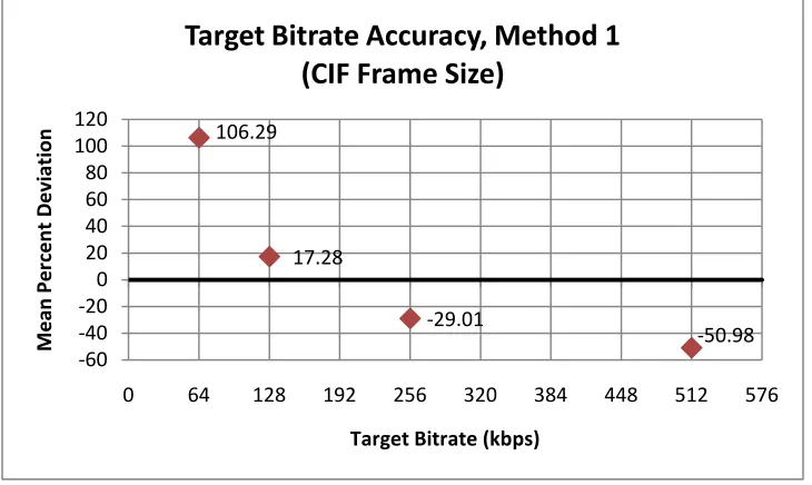
Figure 5.13 Method 1 Target Bitrate Accuracy ... 69
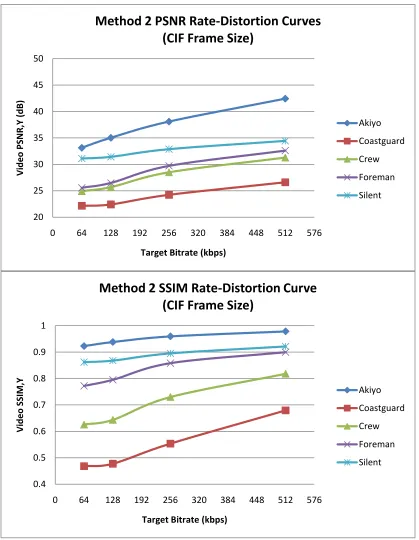
Figure 5.14 Rate-Distortion Curves for Method 2 ... 70
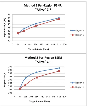
Figure 5.15 Method 2 Per-Region Distortion for CIF "Akiyo" Video ... 71
Figure 5.16 Method 2 Per-Region Distortion for CIF “Foreman” Video ... 72
Figure 5.17 Method 2 Target Bitrate Accuracy ... 73
Figure 5.18 Rate-Distortion Curves for Method 3 ... 74
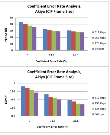
Figure 5.19 Method 3 Per-Region Distortion for "Akiyo" CIF Video ... 75
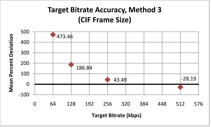
Figure 5.20 Method 3 Target Bitrate Accuracy ... 76
Figure 5.21 Baseline Coefficient Error Response, "Akiyo” CIF ... 78
Figure 5.22 Baseline Coefficient Error Response, "Foreman” CIF ... 79
Figure 5.23 Baseline Motion Error Response, "Akiyo" CIF ... 80
Figure 5.24 Baseline Motion Error Response, "Foreman" CIF ... 81
vi
Figure 5.26 Rate-Distortion Comparison, Method 4 vs. Control Group ... 85
Figure 5.27 Method 4 Blocking and Background Artifacts (CIF Akiyo, Frame 30) ... 86
Figure 5.28 Method 4 Coefficient Error Response, “Akiyo” CIF ... 87
Figure 5.29 Method 4 Coefficient Error Response, "Foreman” CIF ... 88
Figure 5.30 Method 4 Coefficient Error Resilience, CIF "Akiyo," Frame 30, 512 kbps ... 89
Figure 5.31 Method 4 Coefficient Error Resilience, CIF "Foreman," Frame 60, 512 kbps ... 90
Figure 5.32 Method 4 Motion Error Response, "Akiyo" CIF... 91
Figure 5.33 Method 4 Motion Error Response, "Foreman" CIF ... 92
Figure 5.34 Method 4 Motion Error Resilience, CIF “Foreman,” Frame 30, 512 kbps ... 93
Figure 5.35 Method 5 Coefficient Error Response, "Akiyo” QCIF ... 94
Figure 5.36 Method 5 Coefficient Error Response, "Foreman” CIF ... 95
Figure 5.37 Method 5 Motion Error Response, "Akiyo" QCIF ... 96
Figure 5.38 Method 5 Motion Error Response, "Foreman" CIF ... 97
Figure 5.39 Method 6 Coefficient Error Response, "Akiyo" QCIF ... 98
Figure 5.40 Method 6 Coefficient Error Response, "Foreman" QCIF ... 99
Figure 5.41 Method 6 Motion Error Response, "Akiyo" QCIF ... 100
vii
List of Tables
Table 2-1 H.264 Macroblock-to-Slice-Group Mappings ... 14
Table 3-1 Supported H.264 Levels ... 33
Table 3-2 Baseline Modification Results ... 35
Table 3-3 Error Insertion Pseudocode ... 38
viii
Glossary of Terms
Baseline
An H.264 profile that includes low-complexity coding features as well
as error-resilience tools
B-Frame
A video frame that is decoded using Inter prediction from one or more
reference frames
BU
Basic Unit, the smallest piece of video on which H.264 rate control
may operate
CABAC
Context-Adaptive Binary Arithmetic Coding, a high-complexity H.264
entropy coding technique
CAVLC
Context-Adaptive Variable Length Coding, an H.264 entropy coding
technique
CIF
Common Intermediate Format, a video resolution of 352x288 pixels
CODEC
Encoder/Decoder pair
Coefficient
An element of the output matrix of the Discrete Cosine Transform
CPB
Coded Picture Block, a syntax element describing commonly occurring
patterns in transform coefficients
DCT
Discrete Cosine Transform, a matrix transform common to modern
video CODECs
DPB
Decoded Picture Buffer, a storage location for reconstructed frames
DPCM
Differential Pulse-Code Modulation, a form of signal encoder that uses
traditional Pulse-Code Modulation techniques coupled with prediction
Extended
An H.264 profile that is an extension of the Baseline Profile
FMO
Flexible Macroblock Ordering, an H.264 Baseline Profile
error-resilience technique
GOP
Group of Pictures, a set of one or more frames in display order
High
An H.264 profile that includes high-complexity extensions for high
ix
I-Frame
A video frame that is decoded using only Intra prediction
Inter Prediction
A prediction method using available samples from within previous
reference frames
Intra Prediction
A prediction method using available samples only from within the
same frame
IPCM
A lossless macroblock coding mode in which pixel data is transmitted
directly
JM
Joint Model, an open-source H.264 implementation provided by the
JVT
JVT
Joint Video Team, the standards group responsible for H.264,
consisting of members of both MPEG and VCEG
Level
A set of performance requirements for decoding a video, used to
specify encoder and decoder compliance
Macroblock
A 16x16 block of pixels within a video frame
MAD
Mean Absolute Difference, a distortion metric used at the frame and
macroblock levels
MSE
Mean Squared Error, a distortion metric used at the frame and
macroblock levels
Main
An H.264 profile that includes more computationally intense features
than Baseline, but lacks error resilience tools
MB
Macroblock, a 16x16 pixel piece of a video frame
Motion Vector
A 2-d vector specifying the relative motion of one macroblock or
macroblock partition to its reference, used in Inter prediction
MPEG
Moving Picture Experts Group, a video compression standards
committee under the International Organization for Standardization
NAL
Network Abstraction Layer, a process by which the encoded H.264
bitstream is translated into byte-aligned packets
P-Frame
A video frame that is decoded using Inter prediction from a single
x
PPS
Picture Parameter Set, an H.264 syntax element that specifies video
coding parameters for one or more frames
Profile
A specific subset of the H.264 bitstream, used to specify encoder and
decoder compliance
PSNR
Peak Signal-to-Noise ratio, an objective measure of video quality
QCIF
Quarter Common Intermediate Format, a video resolution of 176x144
pixels
QP
Quantization Parameter, a value expressing the amount of quality to
be removed during the quantization process; varies from 1 to 51 in
Baseline Profile H.264
Rate Control
Video coding algorithms utilized to achieve a target bitrate for
decoding or transmission
RDO
Rate-Distortion Optimization, a computationally intense process used
to select a prediction mode by balancing bitrate and distortion
Residual
The result of subtracting a predicted macroblock from its reference
RoI
Region of Interest
Slice
One or more macroblocks; the smallest unit in which compressed
pixel information can be sent using NAL coding
Slice Group
A subset of all of the macroblocks within a frame, used to partition a
frame into regions
SPS
Sequence Parameter Set, an H.264 syntax element that specifies video
coding parameters for an entire video sequence
SSIM
Structural Similarity Index, an objective measure of video quality
YCbCr
A color space typically used in video coding; analogous to YUV, but
implies digital encoding
YUV
A color space typically used in video coding, with Y representing
luminance and U, V representing blue and red chrominance
VCEG
Video Coding Experts Group, a video compression standards
1
Chapter 1
Introduction
1.1.
Motivation for Low-Bitrate, Low-Complexity Region of Interest Coding
Since its inception in 2003, the H.264 video coding standard has become one of the most robust Discrete Cosine Transform (DCT) based video compression specifications. Several features have been added as annexes to the standard, including Scalable Video Coding and Multiview (3-D) coding extensions. There has also been much work in the field of H.264 Region of Interest coding; however, no techniques have yet emerged as part of the draft model. As the number of computing resources available to smaller devices continues to increase, so too do efforts to implement low-complexity H.264 CODECs for use in real-time mobile video coding and similar applications.
Though there has been much research in both of these areas, little has been done to combine them. As low-complexity video coding often utilizes wireless transmission channels, which support much smaller bandwidths than wired media and boast greatly varying error rates, Region of Interest coding may be applied to great effect by increasing the error resilience of important pieces of a video. RoI coding may also be used to allocate a larger part of the bandwidth to these regions. Using either technique often requires tradeoffs between computational requirements, video quality, and bandwidth utilization. This thesis project sought to examine those tradeoffs.
1.2.
H.264 Advanced Video Coding
2
Figure 1.1 H.264 CODEC Block Diagram
H.264 processes videos frame-by-frame, where each frame is then broken up into macroblocks – discrete 16x16 pixel regions. As H.264 operates in the YCbCr color space, each macroblock contains both luma and chroma pixel values. Figure 1.1 shows the various major elements of an H.264 CODEC, and the processing that each macroblock undergoes during the encoding and decoding processes. The major encoding elements are each described briefly below.
The first stage of encoding in an H.264 CODEC is known as prediction. Before a macroblock can be processed, an encoder must select its prediction model; H.264 contains two primary modes. They are Intra, in which the pixels of a macroblock are constructed by utilizing samples from neighboring blocks within the same frame, and Inter, in which the pixel values are computed using samples from previously coded frames. Each of these modes has several options, leading to a large number of possible values. The end goal of this first phase is to allow the predicted macroblocks to be as close as possible to the corresponding original blocks, using information available to the decoder. After the pixel values are calculated at the first stage, a residual block is computed as the difference between the original macroblock and the predicted block. The closer this residual is to zero, the higher compression attainable for the macroblock. For all cases, prediction is a lossless process.
3
frequency domain, where low-frequency (DC) components tend to carry higher importance than higher-frequency (AC) components; actual importance of higher-frequency depends on the properties of the input video. The exact transform used depends on a number of factors, including whether luma or chroma values are being transformed and which prediction mode was used. As with prediction, transformation is a lossless process.
Following transformation, the coefficients are reduced in magnitude during quantization, the only lossy compression process within H.264. Quantization operates via a single parameter – QP – that determines the scaling factor for the coefficients. QP can be provided as a fixed input parameter, or may be calculated via rate control, a process that is described in Section 2.1.
After being quantized, coefficients are given an ordering for later transmission. This reordering places coefficients in order of importance, with the DC component in the top-left of the coefficient matrix first and the highest-frequency AC component in the bottom-right of the matrix last. It is commonly known for the zigzag pattern that it traverses.
The final compression process, known as entropy coding, is a more traditional form of compression. It utilizes variable-length codes to represent commonly-occurring pixel patterns and bitstrings with fewer bits. H.264 uses three different forms of entropy coding: Context-Adaptive Binary Arithmetic Coding (CABAC), Context-Adaptive Variable Length Coding (CAVLC), and Exp-Golomb coding. The choice of coding type depends on which syntax element is being processed, as well as computational requirements – CABAC is more complex, but can provide higher compression ratios, for example.
H.264 includes one additional layer of encoding, known as the Network Abstraction Layer, or NAL. The NAL processes the output of the entropy coder and combines various parts of the H.264 bitstream into byte-aligned NAL units that are more amenable to packet-switched networks. For example, all macroblocks in a single slice are transmitted as a single NAL unit.
4
reconstructed macroblocks are stored in the Decoded Picture Buffer (DPB) until they are no longer needed as references.
For more information on H.264 encoding and decoding, refer to [1] and [2].
1.3.
H.264 Profiles and Levels
5
Figure 1.2 Features of the H.264 Baseline, Extended, Main, and High Profiles [3]
Figure 1.2 describes the four major profiles of H.264. The Main and High profiles are typically used in high-resolution and high-quality video, and are not generally suitable for real-time video coding. The Baseline and Extended profiles remove several features with higher computational requirements, and add several error resilience tools. This project focused primarily on the Baseline profile, which is particularly well-suited to low-complexity platforms.
1.4.
Region of Interest Coding in H.264
6
the quality of one or more specific regions. This is the goal of Region of Interest coding. Several techniques are available for RoI coding in H.264, and several of these are applicable specifically to low complexity H.264 implementations, and are ideal for computationally limited platforms.
Figure 1.3 Typical Region of Interest Incorporating Subject's Face
With H.264, there are two major tradeoffs that may be exploited when considering Region of Interest coding. The first is the tradeoff between quality and bitrate – for a given video sequence, the amount of quantization may be increased to reduce the bitrate of the video at the expense of quality. Region of interest coding may instead reallocate bits from the background to the region(s) of interest, increasing quantization in the background and decreasing it in the foreground. Doing so will increase the quality of the foreground, possibly making the video appear of higher quality to a human observer. For example, human observers have been found to focus on areas of a video that contain faces and hands. If the region of interest includes these areas, as in Figure 1.3, subjective video quality may be improved. Such region of interest techniques must by necessity target the rate controller when implemented in H.264.
7
not the background, which may be far more effective at preserving RoI quality when a high error rate is present.
This thesis project selected RoI coding techniques from both categories, specifically targeting those that were deemed applicable to both low-complexity and low-bitrate or error-prone environments.
1.5.
H.264 JM Reference Software
In addition to drafting a standard for the H.264 bitstream, the JVT has designed and implemented a reference H.264 CODEC in the form of the JM Reference Software. It is one of the most fully-featured H.264 CODECs available, and has the added benefit of using the same terminology in its code as the H.264 standard document.
The JM Reference Software implementation includes all H.264 profiles and levels, and has been updated to include the Scalable Video Coding and Multiview Coding extensions as well. It does, however, perform much more slowly than other implementations [4].
This project utilized the JM Reference Software as the foundation for its implementation and testing. The code was modified by stripping out all non-Baseline features, and further outfitted with error modeling and region of interest coding features. These code modifications are described in Chapter 3.
1.6.
Project Goals & Assumptions
As previously stated, this project’s motive was to investigate low-complexity Region of Interest coding techniques that are applicable to low-bitrate and error-prone scenarios. The term “low bitrate” is used to mean any encoded video bitstream that requires approximately 256 kbps or less to transmit at some specific framerate. “Error-prone” is used to describe a transmission channel that is likely to lose packets of data. These two definitions form the basis of several assumptions for the project, namely the RoI coding methods selected, their implementation, and the parameters chosen for the experiments performed.
8
CODEC performance, methods targeting these functions were eliminated from the investigation. Furthermore, methods utilizing non-Baseline Profile features, such as weighted prediction, bi-prediction, and subpixel interpolation, were also excluded.
9
Chapter 2
Theory
2.1.
H.264 Rate Control Model
Rate control in video coding is designed to address two issues – limitations on transmission speeds, and decoder buffering. If transmission channels cannot handle the volume of video data at a sufficient rate, then significant buffering will be required when decoding. Similarly, it is desirable to avoid the decoder’s buffer becoming too full or from emptying, causing the decoding process to stall waiting for data. If all of these requirements are met, then near-real-time video coding becomes possible, a common goal in low complexity scenarios. The rate control model for the JM Reference Software is specified primarily in the document JVT-G012-r1 [6]. Note that the H.264 standard places no constraints on rate control, and simply provides guidance to aid in implementation. The following model is the default rate control model included in the JM.
The fundamental goal of rate control then becomes meeting the target bitrate. Knowing this bitrate, which may be constant or time-varying, and the framerate of the video being processed, an encoder may generate bit targets for various parts of the video sequence. Rate control in H.264 operates under several assumptions, the first of which are the properties of video rate-distortion curves.
10
Figure 2.1 Typical Rate-Quantization Curve
Over the course of a video sequence, the complexity of frames may vary drastically. Complexity can be defined either as variation across a single frame or variation across multiple frames (i.e. fast motion). As source complexity varies, the rate-quantization curve will shift, as shown in Figure 2.2.
Figure 2.2 Rate-Quantization Curve with Varying Source Complexity
11
(2-1)
In (2-1), Bits represents the number of bits for the entity being coded (typically a frame), MAD is the Mean Absolute Difference (used to measure distortion) between two entities, and C1 and C2 are coefficients updated for each entity. In H.264, the bit target can apply only for residual bits; a certain number of bits will always be required by header elements.
To ensure that the decoder’s buffer requirements are met, the rate controller employs a fluid flow traffic model as well. This model assumes a given number of bits will be removed from the buffer for each frame that is processed, and uses both the number of bits in the buffer and a target buffer level to determine bit budgets at each level of rate control.
A problem arises in the availability of the mean absolute difference. H.264 encoders typically employ a technique known as Rate-Distortion Optimization, or RDO, to select a prediction mode. RDO attempts to encode a macroblock using each prediction mode, and selects the mode which minimizes a set of cost functions. These cost functions describe the tradeoff between bitrate and video quality. To solve the cost functions, RDO requires that a QP be specified, and provides a value for mean absolute difference. Meanwhile, the rate controller requires a MAD to compute bit targets, and provides a QP. This scenario creates what is known as the “chicken-and-egg dilemma,” and is solved in the rate controller by predicting the MAD using a linear model.
12
Figure 2.3 Layers of Rate Control in H.264
A frame may be further divided into basic units (BUs). A BU may consist of one or more macroblocks, with the only restriction that the number of macroblocks in a BU be an integer divisor of the number of macroblocks within a frame. To the rate controller, basic units are indivisible; each BU that is processed receives a single QP value, and all macroblocks within the BU are processed with that parameter.
Use of the basic unit layer in the JM rate control model replaces the frame-layer model, with two exceptions. First, the initial frame in each GOP (which is always an I-Frame) is always coded using a single quantization parameter. The P-Frame immediately following it is also coded entirely using that same QP. Second, all B-Frames are coded using a fixed QP, calculated at the frame level. As B-Frames were not utilized for this project, they will not be discussed in detail here. All remaining P-frames are processed at the basic unit level, by calculating a frame’s bit budget normally and dividing it evenly among all BU’s in the frame.
13
complete the GOP, a number of frames following it are “skipped” until the rate controller estimates that the budget will be met again. H.264 possesses special skip prediction modes, in which no macroblock data needs to be transmitted. A decoder encountering a skipped macroblock will assume an algorithmically-determined prediction mode and a residual of zero for the macroblock. This has the effect of generating less than 1 bit per skipped macroblock; the encoder has to transmit only the number of macroblocks that have been skipped. If a frame’s bit budget is exceeded by any of its BUs, the rate controller will increase the QP for all remaining BUs in the frame.
The QP provided by the rate controller is subject to two further limitations. QP that varies too much from frame to frame can cause large variance in visual quality that is noticeable to human observers. To avoid this, the JM rate control model limits the QP of a frame to within ±2 of the previous frame’s QP. Similarly, blocking artifacts can occur between neighboring BUs if the QP delta between them is too large, and the rate controller places limits on this as well. The QP is also bounded between its minimum and maximum values, which in H.264 are 1 and 51, respectively.
As rate control normally uses floating-point operations, in an embedded environment the rate controller is best targeted for an embedded processor, where fixed- or floating-point ALUs are more likely to be available. Use of RC does not generally add significant delay to the encoding process, and as such it is not a good target for hardware acceleration.
2.2.
H.264 Flexible Macroblock Ordering Techniques
The H.264 Baseline Profile includes several tools for adding error resilience to an encoded bitstream. Of these, only one lends itself readily to RoI coding. Flexible Macroblock Ordering (FMO) provides a means of partitioning video frames into regions, known as slice groups. A slice group, like a slice, is a subset of the macroblocks within a video frame. However, slice groups may also consist of one or more slices. When FMO is in use, each macroblock in the frame is assigned a slice group ID number, and all macroblocks within each slice group are transmitted together. The only other requirement is that macroblocks be transmitted in raster order within a slice.
14
of FMO) is determined by the FMO mode that is in use. H.264 as a standard specifies six specialized macroblock-to-slice-group modes, plus a seventh explicit mode that allows any customized mapping.
Table 2-1 H.264 Macroblock-to-Slice-Group Mappings
Type Name Max. Slice Groups Description
0 Interleaved N N macroblocks are assigned to each of M slice
groups, in round-robin order
1 Dispersed N Macroblocks within each group are dispersed
throughout the picture, in an approximation of a checkerboard pattern
2 Foreground/Background N N rectangular overlapping/non-overlapping regions are each assigned a slice group, with the remainder (background) allocated to another group
3 Box-Out 2 A box of specified size is created by starting from the center and spiraling outward. Group 0 is assigned this box; group 1 is assigned all others.
4 Raster Scan 2 Group 0 is assigned the first M macroblocks in
raster scan order; group 1 is assigned all others.
5 Wipe 2 Group 0 is assigned the first M macroblocks in
vertical scan order; group 1 is assigned all others.
6 Explicit N Each macroblock is explicitly assigned a slice group ID.
15
Of these seven mappings, only two are truly of interest for Region of Interest coding: the foreground/background and explicit mappings. Both allow useful RoI shapes to be constructed. The foreground/background mapping type restricts regions to rectangles, but requires fewer overhead bits to transmit the mapping. As only the locations of the top-left and bottom-right macroblocks for each foreground region are required, the total number of values that must be transmitted for map type 2 is 2(N-1), where N is the number of slice groups. The explicit mapping type allows any arbitrary shape (limited to macroblock resolution) but requires more bits to transmit, as each macroblock requires its own slice group ID. The size of the mapping is therefore NMBFrame, the number of macroblocks in a frame. The exact number of bits required for each mapping is unknown, as each value utilizes an Exp-Golomb variable-length code during transmission.
Figure 2.4 Example Foreground/Background FMO Mapping [3]
As H.264 bitstreams allow the transmission of multiple picture parameter sets, the transmission of several FMO mappings is possible. Each will incur the overhead penalty of a full PPS, as opposed to just the mapping. In addition, H.264 allows a maximum PPS ID value of 255, limiting the number of mappings. This effectively disallows frame-by-frame RoI tracking (which would be inefficient as well) without breaking the constraints of the standard.
2.3.
Video Distortion Modeling
16
PSNR, or Peak Signal-to-Noise Ratio, is the most commonly-used objective metric for video distortion. It is defined in terms of the maximum pixel value and the Mean Squared Error (MSE) between two video frames. Similar to other SNRs, it is expressed on a logarithmic scale. (2-2) and (2-3) provide the definition for video PSNR.
(2-2)
Where
(2-3)
with F1 and F2 representing the two frames being compared, and pixelmax2 is the maximum pixel value, squared. To extend this definition to include an entire video sequence, the PSNR value of all frames is simply averaged. Additionally, PSNR does not specify whether luma or chroma values are being considered, thus PSNR can be computed for the Y, Cr, and Cb components separately, and also as a whole. For most video sequences, Y PSNR is the best indicator of video quality, second to including both chrominance values as well. One notable problem with PSNR is that it approaches infinity as the frames approach equality, and is undefined for equal frames.
More recently Structural Similarity Index, or SSIM, has also been adopted as an additional objective metric. Though it typically only considers luma values, SSIM is generally thought to be a better indicator of human preference for video quality than PSNR. This is due to the fact that it considers variances within both pixels in both frames, as well as the covariance between frames. It also operates on a much smaller window size than a full frame, typically 8x8 pixels, and allows the windows to overlap, considering all possible windows within the frame. Equation (2-4) describes how to compute SSIM.
(2-4)
17
constants used to balance the ratio should the denominator become too small; their values are based on the maximum squared pixel value.
SSIM ranges from -1.0 to +1.0, with +1.0 representing two identical windows. SSIM for two frames is simply the average of the SSIM of all windows in the frames, and SSIM for a video sequence is likewise the average SSIM of all its frames.
Though very computationally intense, SSIM has been shown to correlate more strongly with human perception [7], and as such SSIM values have been included in all experiments conducted for this project, in addition to PSNR values for Y, Cr, Cb, and their combined results. However, a more accurate measure in terms of Region of Interest coding would also consider the PSNR and SSIM of each region. As no software was available to do so, and the JM Reference Software included no such model, a custom implementation was created that could compute required PSNR and SSIM values. The software is described in more detail in Section 3.3.
2.4.
Selected RoI Coding Techniques
This thesis project sought to examine low-complexity RoI coding techniques that were thought to be suitable for operating in low-bitrate or error-prone environments. To this end, several different coding techniques were selected from various research sources. These methods are best split into two categories, as discussed in Section 1.4: those that focus solely on video quality (quantization and rate control), and those that focus on error resilience. The theory behind each technique will be discussed in detail below.
2.4.1
Method 1 – Maximum Bit Transfer
This method, presented in [8], provides a simplified rate control model as a means of allocating bits from background macroblocks to foreground macroblocks. As the original method was created targeting H.263, the predecessor to H.264, it has been updated here to reflect the changes made to the JM rate control model – namely, the basic unit layer.
Method 1 specifies a simple principle for bit reallocation: use the maximum amount of quantization on background MBs, and transfer the bit savings to the foreground. The equation is presented as:
18
In (2-5), h represents the number of bits required for encoding header information, Bf and Bb represent bits required by the foreground and background, respectively, and QPf and QPb represent the corresponding quantization parameters. BMBT is the bit budget for a frame. MBT operates by setting QPb = QPMAX = 51, and solving for the bits remaining for the foreground. The authors of [8] propose an iterative method to solve for QPf, in which the QP is set to QPMAX and steadily decreased until the difference between the new bit budget and the original has been minimized. However, this technique is computationally intense, as each iteration requires several floating-point operations. Furthermore, it does not leverage H.264’s use of basic units to apply a finer grain of rate control. As such, the following modifications were made:
For the initial I and P frames of each GOP, set the quantization parameter of all background MBs to the maximum value. Set the foreground QP to the initial QP determined by the GOP, which is typically low. Tests on several video sequences showed this to yield sufficiently close bit budgets, without significant spikes in the bitrate, and also excluding the additional iterations, each of which would require the use of the quadratic rate-quantization model.
For all following frames, require that basic unit size be exactly one macroblock. If a basic unit (macroblock) is located within the background, set its quantization value to QPMAX. Otherwise, allow the rate controller to calculate a bit budget for each BU manually. The reduction in bits from the background macroblocks will automatically translate to lower QPs in the foreground, and the bit budget for the frame will be met more closely than at the frame level.
As this technique violates the constraints placed on QP variance, these constraints were removed for Method 1.
2.4.2
Method 2 – Content-Based Bit Allocation
Described in [9], Method 2 provides a multifaceted approach to bit reallocation from background to foreground. It uses information on both the relative size and motion of each region relative to the whole frame, and also allows variable priority to be given to the RoI. The technique was originally designed for use in H.261, where it operated at the frame layer, but it can be extended to work at the frame layer or the basic unit layer, depending on the settings provided to the encoder.
19
region, based on two factors – size and motion. The size is simply the ratio of the number of macroblocks in a region to the number of macroblocks per frame, as shown in (2-6).
(2-6)
Above, Nmbf represents the number of macroblocks in the foreground, Nmbb represents the number of macroblocks in the background, and Nmbframe represents the number of macroblocks in each frame. The algorithm also considers the motion of each region, in terms of its motion vectors after prediction:
(2-7)
In (2-7), Mf represents the sum of the magnitude of all motion vectors in the foreground over the sum of the magnitudes of all motion vectors in the frame; Mb represents the same ratio for the background.
Once the bit budget BT for a frame has been established, the budget may be distributed between foreground and background macroblocks using (2-8).
(2-8)
20
(2-9)
P is a ratio, from 0 to 1, determining the proportion of bits to reallocate. It can be thought of as the amount of priority to give the RoI.
Because this method was originally designed for H.261, it does not allow the same granularity as H.264 rate control. However, the equations above all translate easily to the basic unit layer in H.264. Simply replace “frame” with “basic unit,” and the adaptation is complete. Each basic unit is processed in the same manner by the algorithm: an initial bit budget for the BU is determined, the size and motion of the foreground and background in the BU is determined, and bits are reallocated from foreground to background MBs accordingly. Once this step is complete, QPs can be calculated using the quadratic model described in (2-1) and each macroblock in the BU can be coded.
One final modification can be made to the algorithm. Because changing QP too rapidly can cause significant blocking artifacts, maximum and minimum bounds may be placed on the change in QP from macroblock to macroblock. In the JM Reference implementation, a maximum delta QP of 2 is specified; this implementation, like Method 1’s implementation, removes the constraint. QP values must still be clipped within the range [1, 51], however.
In terms of complexity, this method does not add significant requirements to the existing H.264 rate control algorithm. The main computations being added are in the motion vector summations, which generally aren’t already done by an encoder. This, along with the extra computations to reassign bits from background to foreground and memory accesses to check whether an MB is in the background or foreground, are the only significant additions to both time delay and computational complexity.
2.4.3
Method 3 – Multiple-Priority RoI Coding
21
method is capable of automatically handling several RoI shapes, including rectangular, circular, and a “foveated” shape that is based on the shape of the human retina.
The method specifically targets a two-layer approach to Rate Control. This means that it does not consider basic units at all, only assigning bits at the GOP and frame levels. At the GOP layer, the modified bit budget for a given GOP is computed as:
(2-10)
QPi,j(1) represents the initial QP assigned to the ith GOP, for the jth priority level. SumPQP represents the sum of the QP of all P pictures in the ith GOP, jth priority level. N and NP represent the number of frames and the number of P-frames in the GOP, respectively. (2-10) assigns the initial QP for a GOP based on the number of frames in the previous GOP and their QPs, and clips the result to within ±2 of the previous GOP’s initial QP.
At the frame level, [10] recommends using the same linear MAD prediction model utilized by H.264’s rate control algorithm, as well as the same quadratic model for QP computation. Bit distribution among priority regions is calculated using (2-11), below.
(2-11)
Si,j(k) is the relative size of the jth region, in frame k of the ith GOP, MADi,j(k) is the normalized predicted MAD of the region, and ws and wMAD are weighting factors that influence the importance of size or distortion respectively, with the constraint that ws + wMAD = 1.
22
same principle is applied to the quadratic model used to calculate QP, with each region receiving its own model parameters.
To calculate bit reallocation, a priority constant P0 is used. This constant can be supplied as an input, and is used to calculate the priority of all n-1 remaining regions, with the highest priority region being given priority P0, using (2-12).
(2-12)
Finally, a bit target can be assigned to each region using (2-13):
(2-13)
Once the target bits are known, the target QP can be computed and rate control proceeds normally.
From a complexity standpoint, Method 3 requires more resources than Methods 1 or 2. It allocates additional storage for the linear and quadratic models for each priority region, and also requires several more calculations – one per region, rather than one for the frame. However, since this method replaces the traditional H.264 basic unit layer, it can be thought of as roughly analogous to the JM rate control implementation, with N basic units per frame (where N is the number of priority regions), with a few extra computations added for RoI coding – the bit reallocations from foreground to background, for example. It was expected that the quality difference, especially in terms of human perception rather than PSNR, would be noticeable between Method 3 and Methods 1 or 2, due to the smoothing out of the QP changes from foreground to background.
2.4.4
Method 4 – Error Resilience via Nonlinear Transform
The authors of [11] have proposed the first technique selected by this project as an RoI method targeting error resilience. As opposed to reallocating bits through modifications of QP, this method instead aims to improve the error resilience of macroblocks within the RoI through redundancy.
23
video sequence to contain the redundant RoI. A nonlinear transform is applied to this effect, such that the encoder and decoder may have no knowledge that the RoI method is in use. This project limited the method to overwriting background macroblocks, and did not consider cases where the frame size was expanded. Figure 2.5 shows an example of an image before and after the transform is applied. Note that not only are RoI macroblocks copied to replace background macroblocks, the background that is being replaced is “squeezed” so as not to lose too much background information.
Figure 2.5 Example of Nonlinear Transform with Background Loss
The authors of [11] recommend an RoI tracking technique to use in conjunction with this method; however, as RoI tracking was not the focus of this project, no tracking method was utilized. Support for a mobile RoI with this technique is allowed, and was implemented in the modified software in a similar manner to FMO slice groups, with a maximum of one mapping per frame. This particular method limits the RoI shape to a rectangle, and so the RoI specification was further limited in the modified software to slice group mapping type 2 (foreground/background) with two slice groups.
24
the original frame. Furthermore, the values xns,RoI and yns,RoI correspond to the starting positions of the RoI in the transformed frame. In effect, every macroblock in the original frame becomes a pair of macroblocks in the transformed frame, displacing the background and causing it to “shrink” to fit within the altered frame. Though the pair of macroblocks will not perfectly replace each other (due to different prediction methods being selected, for example) the correlation between them would likely be high enough that one could be used to replace the other with little mismatch. In [11], correlations between 0.88 and 0.98 were reported, with 1.00 representing a perfect match.
(2-14)
The corresponding inverse transform is given in (2-15).
(2-15)
The paper also introduced an error concealment method, should data be lost in either the foreground or background. In the interest of comparing the error resilience of this method to the other methods, no error concealment was implemented, except to replace a lost RoI macroblock with its redundant “twin.” This process, rather than attempting error concealment at the decoder, used the reconstructed output frames from the encoder.
25
work could be offloaded to a separate hardware or software unit, if desired. The technique is more effective than simply transmitting slices redundantly, especially when the RoI is considered, because it does not need to retransmit entire frames, and in fact will transmit no more information than would appear in a single frame. The biggest disadvantage is that this technique requires that additional work be done before encoding and after decoding, meaning that the postprocessor must be present to recover the original video frames after decoding is complete. Background quality will also suffer degradation, even with zero errors in the bitstream, should Method 4 be enabled without frame size expansion.
2.4.5
Method 5 – RoI Coding with Flexible Macroblock Ordering
In comparison with the other methods, Method 5 was the least complex in terms of changes required to the JM Reference Software. The reason for this is that it utilizes FMO mapping type 6 (explicit mapping) to define a more complicated mapping for the RoI than for the background. Given the proposed changes to the FMO functionality of the JM software, this method may either support a fixed or a moving RoI, but its efficiency in terms of bitstream overhead increases with the motion of the RoI. Method 5 is specified in [12].
26
Figure 2.6 Advanced FMO Mapping Proposed for Method 5
In the figure, the entire background is placed within one slice group, and is given the highest slice group ID number. The RoI is split into two groups, mapped using the dispersed pattern. The black squares represent macroblocks within slice group 1, and the white squares represent macroblocks within group 0. By transmitting slices out of order in this manner, the error resilience of the RoI is improved, as loss of a single slice (or even a slice group) would at least spatially distribute the errors.
This method’s choice of mapping is of interest in that it provides less efficiency than simply using mapping type 1; the dispersed mapping type transmits only its type information and the number of slice groups, and the encoder and decoder compute the slice group IDs for each macroblock automatically. The primary benefit of this technique is in its ability to distinguish between the RoI and background – the background can be defined as the slice group with the highest ID, and all foreground regions can be found below it, with each pair of IDs belonging to a single rectangular region.
27
control model provides more flexibility and control over the buffer regulation, and Methods 1 and 2 already provide similar functionality.
As stated before, the complexity of this method is minimal, and only requires the precomputation of the mapping for each frame. This precomputation only needs to be performed when the RoI moves, and so for a fixed RoI the mapping is transmitted in the first picture parameter set and the method is finished.
2.4.6
Method 6 – Explicit Spiral Interleaving
The final error resilience RoI method also focuses on Flexible Macroblock Ordering, but utilizes Redundant Slices as well. Rather than use a combination of FMO mapping types 1 and 2, the authors of [13] propose a combination of types 0 (interleaved) and 3 (spiral) that they term Explicit Spiral Interleaved (ESI). Figure 2.7 provides a basic example.
Figure 2.7 Explicit Spiral Interleave (ESI) FMO Mapping [13]
Slices are ordered using an inward spiral pattern, similar to mapping type 3. The spiral pattern is also broken up using interleaving. The authors selected this pattern as they believed it would result in maximum spatial dispersal should a large number of macroblocks be lost. Spatial dispersal of errors is useful for two reasons – errors in a frame are less noticeable or annoying to human observers if they are dispersed, and error concealment tools are more effective if more neighboring macroblocks are available.
28
One caveat to redundant slices is that the redundant representations are not required to use the same coding parameters as the original slices; they may, for example, use higher quantization to decrease the number of bits in the secondary slices. This does create a discrepancy between the encoder and decoder in the event the decoder needs to replace a missing slice with a redundant slice. Due to the increased complexity of coding the same slice twice using different parameters, this project will only consider the case where redundant slices use the same coding parameters as the corresponding primary slices.
The paper also included a dynamic model for using redundant slices based on the characteristics of the channel. Because this project presupposed no knowledge about the channel, except that it is error-prone and bandwidth-limited, this feature was not included in Method 6. Redundant slices were also unable to be used, as they were not part of the Baseline profile. This method was selected simply to gauge the effectiveness of its FMO mapping versus Method 5’s.
29
Chapter 3
Design
3.1.
Baseline Software Code Modifications
The code changes for this project took place in two phases. The first phase removed all unnecessary elements that increased the size of the code, the size of the executable, and made the code less readable. To complete this phase, all non-Baseline features were removed from the JM Reference Software, version 17.2. Several other features that were not particular to the Baseline Profile but were deemed unnecessary for the projects utilizing the code, including handling of non-YUV videos and H.264 levels used for coding high definition videos, were also removed.
Removing all non-Baseline features reduced the number of modifications that would be required to implement the chosen RoI coding techniques. It also simplified the computations required for RoI coding – for example, by removing the necessity of considering B-frames during encoding. Furthermore, the changes reduced the size of the executable by nearly 40%. This is important from a hardware/software codesign perspective, which future work may consider.
The removal process was approached on a per-feature basis. Each H.264 profile was examined in turn, and features exclusive to that profile that were not used in Baseline were removed. An attempt was made to target higher-complexity features first, and so the removal process first targeted the High Profile, followed by Main, then Extended. As seen in Figure 1.2, all remaining features would then belong to (or be compliant with) the H.264 Baseline Profile.
The following sections detail the specific features that were removed during each phase of the Baseline code modifications.
3.1.1
High Profile Feature Removal
The following features that were part of the High Profile(s) in H.264 have been removed from the JM software:
Video Formats – All support for 4:2:2 and 4:4:4 chroma subsampling were removed, and
30
Monochrome Video – All support for the 4:0:0 subsampling format, in which only luma samples
are provided, was removed. It is unclear why this feature was limited to the High profile, however.
Separate Color Plane Coding – This feature was added alongside 4:4:4 subsampling, allowing each color plane (R, G, and B or Y, Cb, and Cr) to be coded separately. Basically this forced the encoder to afford all three planes the same priority as luma, where in Baseline H.264 the chroma components would take 1/4 the time (at the very maximum) of luma samples. Typically chroma samples take even less time to process, as they are not considered separately for motion estimation.
Intra-Only Profiles – These profiles were defined in addition to the High Profiles, with the purpose of providing low-complexity, high-quality compression. These profiles cannot come close to the compression capabilities of the other H.264 profiles, but they can operate at very fast framerates and do not degrade video quality as much as predictive coding.
Quantization Scaling Matrices – These customizable matrices allowed the QP values for individual samples to be scaled up or down, affording a greater degree of flexibility to the quantization process at the expense of more memory and computational complexity. The scaling matrices could also be adaptively controlled, as described below.
RDOQ – Short for Rate-Distortion-Optimized Quantization, this set of algorithms allowed several
quantizations to be performed for each block, using a different matrix each time. The best one in terms of both quality and compression would be selected, and the algorithm would keep track of its state, allowing it to adapt as the video is processed.
Cr and Cb QP Control – When operating in the YUV color space (i.e. there are no separate color
planes), this feature allows separate control of the Cr and Cb components. Typically chroma is simply quantized at an offset from the luma component. This feature allows a different offset to be applied to each chroma plane.
31
Lossless Predictive Coding – This feature provided a means of coding P- and B- pictures losslessly, in a more advanced way than simply removing quantization. Ordinarily H.264 provides lossless coding in the form of an IPCM mode, in which a macroblock is simply copied over into the bitstream. These features substantially outperform IPCM mode.
MVC – Short for Multiview Video Coding, this set of features was added to the standard along
with the Multiview High and Stereo High profiles. It supports 3D and multi-perspective video coding from two (in the case of Stereo High) or more (in the case of Multiview High) viewing angles. It is easily disabled in the code through the use of preprocessor directives.
3.1.2
Main Profile Feature Removal
A single feature was removed during this stage: CABAC. Short for Context Adaptive Binary Arithmetic Coding, it is an alternative that some syntax elements in H.264 can use – coded coefficients, for example, as opposed to utilizing standard variable-length codes. This feature requires the addition of an arithmetic coding engine, as well as storage of the 400+ context models used to code different syntax elements. Normally, H.264 utilizes CAVLC, for the majority of its syntax elements, and standard Exp-Golomb VLCs for several others.
3.1.3
Extended Profile Feature Removal
The following features that are part of the Extended Profile in H.264 were removed from the JM software:
Interlaced Video Support – This is a set of features that allows interlaced output – the coding of
each frame as two fields, and provides two forms of coding – PicAFF and MBAff, Picture and Macroblock Adaptive Frame-Field Coding, respectively. PicAFF allows each frame to be specified as progressive or interlaced. MBAFF allows each 16-wide by 32-high “macroblock pair” to be coded as (a) a pair of regular macroblocks or (b) a pair of field macroblocks. MBAFF requires substantial changes to certain steps in encoding, including a new zigzag scan for reordering coefficients and different treatment of slices, macroblock availability, and picture ordering.
B-Slices – This feature, known as bi-prediction, has become standard in most DPCM CODECs. It
32
available in P-coded macroblocks, from partitioning to subpixel refinement. It can provide much better compression performance, at the expense of motion estimation (the primary bottleneck in H.264) taking twice as long. This means that it generally isn’t used in real-time video coding.
Weighted Prediction – This is very similar to bi-prediction, but for coded macroblocks. P-coding only uses List 0, and typically allows one reference per MB. Adding Weighted Prediction support allows P-MBs to use two references. A motion vector is formed for each one, and the final predicted motion vector is calculated as the weighted average of these. The feature adds complexity to P-MBs but can provide higher compression.
SI/SP-Slices – These two slice types were created mainly for streaming video, allowing for
efficient random access without affecting the video’s bitrate by a large amount.
Data Partitioning – This is the major error resilience feature that the Baseline Profile does not
include. It allows slices to be split into three partitions: A, B, and C. Partition A contains all of the vital data for the slice, while B and C are of lower priority. A slice can be reconstructed if partition A is error-free and either of partitions B and C are error-free. If additional error protection is supplied to partition A, the resulting bitstream can theoretically handle higher error rates than Baseline H.264.
Hierarchical Coding – This feature is for the most part associated with B-coding, and allows a hierarchy of reference frames to be set up. The typical coding pattern for a Group of Pictures (or GOP, meaning all frames located between two IDR frames) is IDR-P-B-B-…-P-B-B-…-IDR. This option allows further customization of the GOP by specifying a hierarchy for B-frames. B-frames with higher levels receive higher priority. Several modes are possible, with the last being explicit GOP, described below.
Explicit GOP – This feature is also associated with B-coding, and allows input parameters to specify an explicit pattern for how B- and P-macroblocks are coded. Typically a hierarchical coding pattern is used, as described above. It is useful when the specific features of the video being encoded are known ahead of time, such as when high-motion scenes will occur.
3.1.4
Removal of Additional Features
33
Decoder – The decoder executable was removed from the modified code entirely. The decision
to do so was based primarily on the fact that all tasks utilizing the software were interested in encoder performance. A separate code project was created incorporating solely the decoder, with a single code modification made to remove the constraints placed on QP delta.
Levels above 2.0 – These levels were deemed unnecessary for low complexity video coding,
especially in low-bitrate environments. Level 1, the minimum allowed H.264 level, sets a maximum bitrate of 64 Kbps and a maximum resolution of QCIF (176x144) at 15 frames per second. Level 2.0 supports maximum bitrates of 2 Mbps, at resolutions of up to CIF (352x288) at 30 frames per second. Levels above this were required to support bitrates that were outside the scope of this thesis project. Table 3-1 provides a list of all the remaining levels and their parameters.
Table 3-1 Supported H.264 Levels
Level Max MB/second Max MB/frame Max Bitrate (Kbps) Example Resolutions
1.0 1,485 99 64 QCIF @ 15 fps
1b 1,485 99 128 QCIF @ 15 fps
1.1 3,000 396 192 QCIF @ 30 fps
CIF @ 7.5 fps
1.2 6,000 396 384 CIF @ 15.2 fps
1.3 11,880 396 768 CIF @ 30 fps
2.0 11,880 396 2,000 CIF @ 30 fps
Image Processing – These options allowed images to be pre- or post-processed. They were
deemed unnecessary as they increase the size of the code without providing useful video coding features, and can be performed by other software if necessary.
Alternative I/O Formats – The JM Software originally provided support for TIFF and AVI input.
Because the projects using this software only use raw YUV format video, the other formats were removed.
Quantization Offset Matrices – Offset matrices allow explicit definition of the initial
34
Explicit Sequences – This functionality allowed each picture to be ordered explicitly using a configuration file, as opposed to ordering pictures via one of the built-in H.264 settings. The feature was removed because it added unnecessary code and complexity.
3.1.5
Baseline Modification Results
The non-Baseline features of the JM Reference software were estimated to account for approximately 40% of the software. Removing these features, one would expect to see a corresponding decrease in both the size of the source code and the space required by the compiled executable. In gathering these results, the following procedure was used:
1. The size of the original JM software was measured by compiling the encoder executable (lencod.exe) and examining its size.
2. The number of lines of source code in the original software was computed using a script that counted the total number of lines (including comments and whitespace) in all files in the lencod and lcommon directories. The lcommon directory corresponded to code that is common between the encoder and decoder.
3. The software was forked and modified to incorporate only Baseline functionality, by removing all features described above. Rather than delete the appropriate lines of code, all modifications were made by commenting out code, allowing for easy referral to “deleted” code for easily examining and reverting changes. Comments utilized specially-formatted tags.
4. A script was used that stripped out all specially-marked lines of code.
5. The size of the modified JM software was measured by compiling the encoder executable (the only executable in the modified project, also called lencod.exe) and examining its size.
35
The results of the final code size reduction are shown in Table 3-2.
Table 3-2 Baseline Modification Results
Source Code Lines Executable Size
Original Software 104,392 2.10 MB (2,210,816 bytes) Modified Software 60,909 1.30 MB (1,391,616 bytes)
The reduction in source code was about 38.2%, and the reduction in executable size about 41.6%, both of which were close to the initial estimate of 40%.
It should be briefly noted that there were 60,909 lines of code total in the modified software, after removing all additional comments added during the