Rochester Institute of Technology
RIT Scholar Works
Theses Thesis/Dissertation Collections
8-16-2011
Optimizations and applications in head-mounted
video-based eye tracking
Feng Li
Follow this and additional works at:http://scholarworks.rit.edu/theses
This Dissertation is brought to you for free and open access by the Thesis/Dissertation Collections at RIT Scholar Works. It has been accepted for inclusion in Theses by an authorized administrator of RIT Scholar Works. For more information, please [email protected].
Recommended Citation
Optimizations and Applications in Head-Mounted Video-Based Eye
Tracking
by
Feng Li
M.S. Zhejiang University, 2003
A dissertation submitted in partial fulfillment of the requirements for the degree of Doctor of Philosophy in the Chester F. Carlson Center for Imaging Science
Rochester Institute of Technology
August 16, 2011
Signature of the Author
Accepted by
CHESTER F. CARLSON CENTER FOR IMAGING SCIENCE
ROCHESTER INSTITUTE OF TECHNOLOGY
ROCHESTER, NEW YORK
CERTIFICATE OF APPROVAL
Ph.D. DEGREE DISSERTATION
The Ph.D. Degree Dissertation of Feng Li has been examined and approved by the dissertation committee as satisfactory for the
dissertation required for the Ph.D. degree in Imaging Science
Dr. Jeff B. Pelz, dissertation Advisor
Dr. Daniel R. Lawrence
Dr. Carl Salvaggio
Dr. Jinwei Gu
DISSERTATION RELEASE PERMISSON
ROCHESTER INSTITUTE OF TECHNOLOGY
CHESTER F. CARLSON CENTER FOR IMAGING SCIENCE
Title of Dissertation:
Optimizations and Applications in Head-Mounted Video-Based Eye Tracking
I, Feng Li, hereby grant permission to Wallace Memorial Library of R.I.T. to reproduce my thesis in whole or in part. Any reproduction will not be for commercial use or profit.
Signature
i
Optimizations and Applications in Head-Mounted Video-Based Eye
Tracking
by Feng Li
Submitted to the
Chester F. Carlson Center for Imaging Science in partial fulfillment of the requirements
for the Doctor of Philosophy Degree at the Rochester Institute of Technology
Abstract
Video-based eye tracking techniques have become increasingly attractive in many
research fields, such as visual perception and human-computer interface design. The
technique primarily relies on the positional difference between the center of the eye’s pupil
and the first-surface reflection at the cornea, the corneal reflection (CR). This difference
vector is mapped to determine an observer’s point of regard (POR). In current
head-mounted video-based eye trackers, the systems are limited in several aspects, such as
inadequate measurement range and misdetection of eye features (pupil and CR). This
research first proposes a new ‘structured illumination’ configuration, using multiple
IREDs to illuminate the eye, to ensure that eye positions can still be tracked even during
extreme eye movements (up to ±45° horizontally and ±25° vertically). Then eye features
are detected by a two-stage processing approach. First, potential CRs and the pupil are
isolated based on statistical information in an eye image. Second, genuine CRs are
ii
relationship between the offset of the pupil and that of the CR. The optical relationship of
the pupil and CR offsets derived in this thesis can be applied to two typical illumination
configurations – collimated and near-source ones- in the video-based eye tracking system.
The relationships from the optical derivation and that from an experimental measurement
match well.
Two application studies, smooth pursuit dynamics in controlled static (laboratory)
and unconstrained vibrating (car) environments were conducted. In the first study, the
extended stimuli (color photographs subtending 2° and 17°, respectively) were found to
enhance smooth pursuit movements induced by realistic images, and the eye velocity for
tracking a small dot (subtending <0.1°) was saturated at about 64 deg/sec while the
saturation velocity occurred at higher velocities for the extended images. The difference in
gain due to target size was significant between dot and the two extended stimuli, while no
statistical difference existed between the two extended stimuli. In the second study,
twovisual stimuli same as in the first study were used. The visual performance was
impaired dramatically due to the whole body motion in the car, even in the tracking of a
slowly moving target (2 deg/sec); the eye was found not able to perform a pursuit task as
smooth as in the static environment though the unconstrained head motion in the unstable
iii
Acknowledgements
This thesis would not be possible without the invaluable help and support from a
numerous of people.
First and foremost, I would like to thank my thesis advisor Dr. Jeff B Pelz for his
ability to motivate, explain complicated matters and constant support during every stage
of this endeavor. I am fortunate to have had him as a mentor. His dedication towards his
students is rare and greatly appreciated.
I wish to express my gratitude to Dr. Daniel R. Lawrence, Dr. Carl Salvaggio, and Dr.
Jinwei Gu for serving on my thesis committee and reviewing the thesis.
Many people, current and past members of the Visual Perception Laboratory and
Multidisciplinary Vision Research Laboratory at RIT, helped in the development of this
work. I would like to think Dr. Andrew Herbert, Dr. Mitchell R. Rosen, Dr. Sunsan Munn,
Marianne Lipps and Mary Ellen Arndt for their stimulating discussions about both the
thesis work and a vast array of other interesting topics. I would like to thank Christopher
Louten, Monica Cook, Nicholas MacDowell and other undergraduates in the lab for
assisting me in data collection and other matters.
I want to extend my gratitude to the whole Chester F. Carlson Center for Imaging
Science for providing a pleasant and inspiring atmosphere.
I am deeply indebted to my family for all their love and support throughout these
graduate years. My parents and my sister have sacrificed so much to give me an
opportunity to fulfill my dreams. My lovely daughters Emily and Angela brought me
measureless happiness over the past two years. Most important of all, none of this would
have been possible without the tireless love and support of my wife Nan. For this and
iv
Contents
Abstract ... i
Acknowledgements ... iii
List of Figures ... viii
List of Tables ... xvii
Chapter 1
Introduction ... 1
Chapter 2
Statement of Work ... 4
Chapter 3
Optics of the Eye ... 6
3.1 The Cornea ... 7
3.2 The Iris and Pupil ... 9
3.3 The Lens ... 14
3.4 The Retina ... 15
3.5 The Axis of the Eye and Related Terms ... 18
3.6 Paraxial Schematic Eyes ... 21
3.6.1 Gullstrand Number One Exact Eye ... 22
3.6.2 Gullstrand Number Two Simplified Eye ... 24
3.7 Reflections from the Eye ... 28
3.7.1 Bright Pupil and Dark Pupil ... 28
3.7.2 Purkinje Images ... 31
3.7.3 Corneal Reflection ... 35
3.7.4 Reflections from Attachments to the Eye ... 37
Chapter 4
Eye Movements ... 39
v
4.2 Saccade ... 42
4.3 Optokinetic Response (OKR) ... 45
4.4 Vestibular-Ocular Reflex (VOR) ... 46
4.5 Vergence ... 46
Chapter 5
Eye Tracking Techniques and Applications ... 47
5.1 Ideal Properties of an Eye Tracker ... 48
5.2 Electro-Oculography (EOG) ... 50
5.3 Scleral Search Coils ... 51
5.4 Non-Image-Recoding Based Eye Tracking ... 53
5.4.1 Dual Purkinje Image Eye Tracker (DPI) ... 54
5.4.2 Limbus Eye Tracker ... 56
5.5 Video-Based Eye Tracking ... 58
5.5.1 Fundamentals ... 58
5.5.2 Illumination Structure ... 62
5.6 Hybrid Systems ... 68
5.7 Applications in Visual Perception Studies ... 70
Chapter 6
Eye Tracking Optimizations: Key Issues and Possible
Solutions
...
74
6.1 Key Issues in Video-based Eye Tracking ... 74
6.2 Cameras for High Speed Imaging ... 83
6.3 Proposed Illumination Configuration ... 87
6.3.1 Multiple CRs with Temporally Sequential Illumination ... 88
6.3.2 Multiple CRs with Multispectral Imaging ... 89
6.3.3 Multiple CRs with CR Prediction Technique ... 90
6.4 Optimizing Illumination Collection ... 92
6.5 Filtering Strategies in Minimizing Noise ... 94
Chapter 7
Eye Tracking Optimizations: Modeling of Optical
Relationships between Pupil and CR Offsets ... 99
vi
7.2 Collimated Illumination ... 102
7.2.1 Translational Gain ... 102
7.2.2 Rotational Gain ... 103
7.3 Near-Source Illumination ... 105
7.3.1 Translational Gain ... 105
7.3.2 Rotational Gain ... 108
7.4 Gain Values Validation ... 111
Chapter 8
Eye Tracking Optimizations: Structured Illumination and
Eye Feature Detection ... 118
8.1 Background ... 119
8.2 Illumination Configuration ... 121
8.3 Potential CR Detection ... 122
8.4 Pupil Detection ... 124
8.5 Blink Detection ... 128
8.6 CR Prediction ... 130
Chapter 9
Eye Tracking Applications: Smooth Pursuit Dynamics in
Controlled Static Conditions ... 134
9.1 Background ... 135
9.2 General Methods ... 138
9.2.1 Experimental Setup ... 138
9.2.2 Visual Stimuli ... 140
9.2.3 Eye Movement Recording ... 141
9.2.4 Experimental Procedure ... 142
9.2.5 Eye Tracking Data Analysis ... 142
9.3 Experiment 1: Effects of Stimulus Size and Velocity on Smooth Pursuit ... 143
9.3.1 Subjects ... 143
9.3.2 Data Collection ... 144
9.3.3 Results ... 144
9.4 Experiment 2: Effects of Stimulus Size on Pursuit Velocity Limit ... 152
vii
9.4.2 Data Collection ... 153
9.4.3 Results ... 153
9.5 Discussion ... 161
9.5.1 Effect of Target Velocity ... 161
9.5.2 Effect of Stimulus Size ... 162
9.5.3 Limit of Smooth Pursuit Velocity ... 164
Chapter 10
Eye Tracking Applications: Smooth Pursuit Dynamics in
Unconstrained Vibrating Conditions ...166
10.1 Background ... 166
10.1.1 Whole Body Vibration in Vehicles ... 166
10.1.2 Vestibular System ... 169
10.1.3 Visual Research in Body and Display Vibrations ... 171
10.2 Experiment 3: Effect of Whole Body Vibration on Smooth Pursuits in an Unconstrained Condition... 172
10.2.1 Experimental Setup ... 172
10.2.2 Eye-Movement Recording ... 172
10.2.3 Subjects ... 173
10.2.4 Experimental Procedure ... 173
10.3 Eye Tracking Data Analysis ... 174
10.4 Results ... 177
10.5 Discussion ... 183
Chapter 11
Conclusions and Future Work...185
11.1 Eye Tracking Technique Optimizations ... 185
11.2 Eye-Tracking Technique Applications ... 190
viii
List of Figures
Figure 1. Sagittal horizontal section of an adult human eye. PP, posterior pole; AP,
anterior pole; VA, visual axis. Courtesy of Davson, 1990, page 3. ...7
Figure 2. Formation of the entrance and exit pupil. ...10
Figure 3. The relative positions and sizes of the actual, entrance and exit pupil. ... 11
Figure 4. The relationship between the pupil diameter and illumination (Reeve, 1920). A typical office lighting is 120 cd/m2. ...12
Figure 5. The pupil shape viewed obliquely. From Smith, 2003. ...14
Figure 6. Structure of the retina. From Helga Kolb, 2003. ...16
Figure 7. The distribution of the rods and cones in the retina (left eye). From Falk, Brill, and Stork, 1986, p. 153. ...17
Figure 8. The axes of the eye. From Carpenter, 1988. page 14. ...19
Figure 9. Gullstrand Number One Exact Eye. ...22
Figure 10. Gullstrand Number Two Simplified Eye. ...27
Figure 11. Images of bright pupil (a) and dark pupil (b). Images from C.H. Morimoto, 2000...29
Figure 12. Bright and Dark Pupil. From Jason S. Babcock, MS thesis, Rochester Institute of Technology, 2002. ...30
ix
Figure 14. The relative positions and sizes of the four Purkinje images. Image from Hugh Davson, 1962. page 109, Figure 7. ...33
Figure 15. The first and fourth Purkinje images of three illuminators. The brigher images at the top row are P1 and those at the bottom row are P4. Image from http://www.iris-ward.com/_HTM/MEIS/P/1576-MEIS.htm#Top. ...35
Figure 16. Image of an illumination source formed by the cornea (corneal reflection). ...37
Figure 17. Several suction devices or 'caps' used by Yarbus to measure eye movements. Image from Yarbus, 1967, figure 14, 15 and 17. ...38
Figure 18. Parameters of smooth pursuit. Task is to track a step-ramp target. Adapted from Pola and Wyatt, 1991. ...41
Figure 19. Parameters of saccadic eye movements. ...43
Figure 20. Saccades duration as a function of amplitude. Image from Carpenter, 1988. pp 71, Figure 4.2. ...44
Figure 21. Main sequence of saccades. The relationship between peak velocity and amplitude. Image from Carpenter, 1988. pp 72, Figure 4.3 ...45
Figure 22. A subject wearing an EOG apparatus. Image from Metro Vision, www.metrovision.fr. ...50
Figure 23. Scleral search coil technique. Left: coils embedded in a contract lens. Middle: frame setting surround the subject's head which produces a large electromagnetic field. Right: whole system setup. Images from Skalar Medical BV...52
Figure 24. Insertion of the scleral search coil. Images from Skalar Medical BV. ...53
x
Figure 26. Saccades of different sizes recorded simultaneously by the scleral search coil (solid lines) and the Purkinje eye tracker (solid dots) along with their difference vectors (solid lines close to the baseline). Image from Deubel, et al, 1995. ...56
Figure 27. Limbus eye trackers. Left image from Applied Science Laboratories (www.a-s-l.com), right image from Microguide, Inc. (www.eyemove.com) ...57
Figure 28. Eye images before (a) and after (b) a rotational eye movement; the P-CR vector has noticeably changed. Eye images before (c) and after (d) an apparent translational eye movement caused by a camera movement; the P-CR vector has changed only slightly. Images from Kolakowski & Pelz (2006). ...60
Figure 29. The relationship between the P-CR vector and eye rotational angle. Note that the CR always falls on the focal plane of curvature of the cornea. ...61
Figure 30. ASL Eye-Trac 6000 eye tracker. The infrared illumination from the LED is relayed by the visor to shine on the eye. The light reflected by the eye is collected by a solid state sensor (CCD) in the head-mounted module. The visor is coated to reflect the infrared illumination and transmit the visible spectrum. Left image from Applied Science Laboratory, Inc. ...62
Figure 31. Vision 2000 by EL-MAR Inc. Images from EL-MAR Inc. ...64
Figure 32. Eyelink II head-mounted system. Images from Eyelink II user manual. version 1.05, 2002...65
Figure 33. ISCAN eye tracker. Left image from of ISCAN Inc. ...65
Figure 34. IBM BlueEyes. (A) Camera and two sets of LEDs. (B) Pan/tilt base. (C) Bright pupil image. (D) Dark pupil image. (E) Difference image after thresholding. Images from C.H. Morimoto, 1999. ...67
xi
Figure 36. A hybrid system combining the limbus tracker and video-based tracker. Image from Jochen Triesch, 2002. ...69
Figure 37. The painting of "The Unexpected Visitor" and the gaze patterns of the subject given different instructions. Image from Yarbus, 1967. ...72
Figure 38. Eye Tracking head unit with mounted facemask. Image from CHRONOS VISION GmbH, Germany. www.chronos-vision.de/eyetracking. ...75
Figure 39. Observed irregular reflection when the CR falls on the cornea-sclera interface (limbus). ...78
Figure 40. Scene (left) and eye (right) images taken outdoors on a sunny day. ...80
Figure 41. Parallax error for the case when the distance between the eye camera and scene camera is 1.5 inches. From (Li, 2006). ...81
Figure 42. A target moving at 222 pixels/s (left), and 3796 pixels/s (right) is captured by a standard 60Hz camera. The multiple targets seen in the right image is caused by using a slow 60Hz NTSC camera to capture the fast moving target. ...84
Figure 43. A conceptual illustration of the structured illumination (left) and the highlighted CRs and pupil (right). ...87
Figure 44. The HiBall Tracking System. Adapted from www.cs.unc.edu/~tracker/. ...89
Figure 45. A band separation prism with four optical sensors. ...90
Figure 46. CR-prediction technique. Left: original eye position. Right: eye position after a rotational eye movement. Red squares represent the predicted CR positions. ...91
xii
Figure 48. Headgear for the RIT Lightweight Eye Tracker ...93
Figure 49. Blinks removal by thresholding. Original data are outputs from an ISCAN eye tracker. HPOS is the horizontal position of the point of regard (POR). ...96
Figure 50. Eye before (solid) and after (dashed) a translational eye movement. The CR and pupil center move the same amount as the translational eye displacement if the incident rays are collimated; in this case, the translational gain is equal to 1. ...103
Figure 51. Eye before (solid) and after (dashed) a rotational eye movement. The rotational gain is equal to 0.55 if the incident illumination is collimated. Note that the CR after the eye rotates is located in the focal plane of the cornea in the new position. ...104
Figure 52. Eye before (solid) and after (dashed) a translational eye movement when the illumination source is close to the eye. ...106
Figure 53. Translational gain versus position of the illumination source (with respect to the eye). ...107
Figure 54. Eye before (solid) and after (dashed) a rotational eye movement when the illumination source is close to the eye. ...108
Figure 55. Rotational gain versus position of the illumination source (with respect to the eye). ... 111
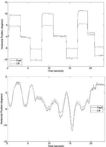
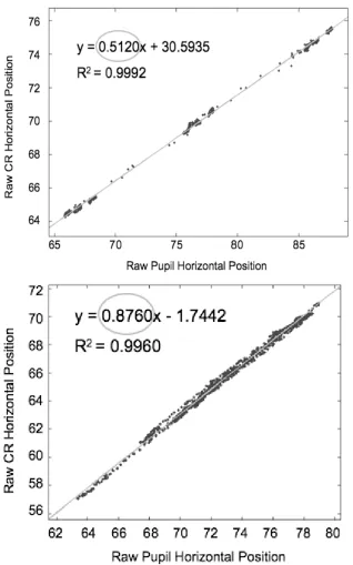
Figure 56. Example data (observer 4) for measuring the rotational gain (top) and translational gain (bottom). Data provided by Kolakowski & Pelz (2006). ... 113
Figure 57. Linear regression for data shown in Figure 56. The overlaid line is the calculated best-fit using least-squares regression, and the slope (circled) of this line is equal to this observer’s rotational (top) or translational (bottom) gain. Data provided by Kolakowski & Pelz (2006)... 114
xiii
possible coupling of eye movements with rotational movements. Using the average gain over five observers provides a better fit (dashed line) than that calculated for this observer (solid line). The subsection of data around a raw pupil position of -20 appears to fall along a line with slope equal to the average rotational gain of the five observers (dotted line). The data were provided by Kolakowski & Pelz (2006). ... 117
Figure 59. Challenging eye images. (a) A CR rolls over to the aspherical part of the cornea; (b) Spurious specular reflections from metal frames in a lift truck (the bright spot below and to the left of the pupil center is the desired CR). Image (b) from D. Giguère at the IRSST - Safety-Ergonomics Research Program, Canada. ... 119
Figure 60. Prototype of the Structured Illumination ...121
Figure 61. Eye images illuminated by the Structured Illumination. (a) The eye looking straight ahead; (b) the eye moved to an extreme position. ...122
Figure 62. Flowchart of the potential CR detection ...123
Figure 63. Eye images in CR detection. (a)(b) Connected components with pixel values in top 1% (highlighted in red color) after eliminating components larger than 0.15% of image size; (c)(d) Potential CRs after the local contrast technique is applied. ...124
Figure 64. Flowchart of the Pupil detection ...125
Figure 65. Pupil detection ...126
Figure 66. Use of the grayscale in the first valley of the histogram to threshold the eye image ...127
Figure 67. Eye images during a blink. (a) Before the blink – circularity = 0.94; (c) During a blink – circularity = 0.58; (e) At the end of a blink – circularity = 0.26. Images (b) (d) and (f) are their corresponding binary images during pupil detection. ...129
xiv
looking straight ahead; (b) The eye moved to an extreme position. Yellow squares represent predicted CR locations, red crosses represent detected genuine CRs, the cyan ellipse represents the pupil boundary, and the cyan diamond represents the pupil centroid.131
Figure 69. CR prediction for a blurred eye image (due to a rapid eye movement). Note that the upper-right CR has not been detected. ...132
Figure 70. Eye velocity versus target velocity (subject K.C.). At target velocities over 100 deg/sec, eye velocities appear saturated with a large variability. The vertical, solid line at high velocities indicate one SD of velocity variability. Image from Meyer, Lasker, et al. (1985). ...137
Figure 71. Experimental setup and eye tracker. Two core-foam boards shown in the left picture were used to limit the subject’s viewing angle to ±30º. Only the left side of the frontal glass from the reader’s view is coated with an infrared reflective coating; the other side is a regular transparent glass. The camera optics has three degrees of freedom of adjustment to center an eye image. ...139
Figure 72. Setup of the projector, DC motor and three first-surface mirrors. Three first-surface mirrors relayed a stimulus image from the projector to the wall. The mirror array sat in a wood supporter which was driven to spin by a DC motor. The small picture on the left-upper corner shows the setup viewed in an opposite direction. ...140
Figure 73. Three stimulus images. (a) The dot (enlarged for display purpose); (b) The apple; (c) The flower image ...141
Figure 74. An example eye-position trace in Experiment 1. Two thick horizontal lines represented the calibration region of the eye tracker (the most-reliable region). Two thin horizontal lines described the visually coded region (±25°). Two dashed vertical lines depicted a steady-state pursuit segment within which eye-position samples were linearly fitted and its slope (solid, slanted segment) was calculated as the velocity of the smooth pursuit. The slanted parallel lines represented the real target velocity. ...143
xv
Figure 76. Check for normality (Experiment 1) ...146
Figure 77. Check for equal variances (Experiment 1) ...147
Figure 78. Gain versus target velocity (Experiment 1) ...149
Figure 79. Gain versus stimulus (Experiment 1) ...150
Figure 80. Eye velocity versus target velocity in Experiment 1. Error bars represented one standard error. ...152
Figure 81. Check for residual independence (Experiment 2) ...154
Figure 82. Check for normality (Experiment 2) ...154
Figure 83. Check for equal variances (Experiment 2) ...155
Figure 84: Gain versus target velocity (Experiment 2) ...157
Figure 85. Gain versus stimulus (Experiment 2) ...159
Figure 86. Gain versus target velocity after pooling the data sets in two experiments. The dashed lines separate the two data sets. Error bars represented one standard error. ...160
Figure 87. Eye velocity versus target velocity after pooling the data sets in two experiments. The dashed lines separate the two data sets. Error bars represented one standard error. ...161
Figure 88. Six degrees of freedom in WBV...168
xvi
Figure 90. A subject tracking the apple moving at the velocity of 4 deg/sec. (a) the target running on the left of the screen; (2) after 0.83 sec (25 frames); (c) after 1.67 sec (50 frames). The cross represents the eye fixation point in the scene. ...174
Figure 91. An example eye-position trace in Experiment 3. Two dashed vertical lines depicted a stable pursuit segment within which eye-position samples were linearly fitted and a slope (solid, slanted segment) was calculated as the velocity for the smooth pursuit.176
Figure 92. Residual vs. order plot in the study of pursuit eye movements in car ...178
Figure 93. Probability plot of residuals in the study of pursuit eye movements in car ...178
Figure 94. Plot of test for equal variances in the study of pursuit eye movements in car179
Figure 95. Target velocity vs. smooth-pursuit gain for the eye tracking study in car ...181
Figure 96. Target velocity vs. eye velocity in the experiment of pursuit eye movements in car. Error bar represents one standard error from the mean. Error bar in the eye velocity (y-axis) is due to variation within and between the subjects. Error bar in the target velocity (x-axis) is due to measurement error, caused by head movements and vibration in the car. ...182
xvii
List of Tables
Table 1. Angular relationship between the different axes of the eye ...21
Table 2. Gullstrand Number One Exact Eye. The parameters in the parenthesis are for the accommodated eye if they are different from the relaxed eye. Adapted from Grand & Hage, 1980. pp 65-66 and Southall, 1937. pp 57-58. ...23
Table 3. Gullstrand Number Two Simplified Eye. The parameters in parentheses are for the accommodated eye if they are different from the relaxed eye. Adapted from G. Smith and D. Atchison, 1997. pp 778-779. ...26
Table 4. Some symbols used in the Gullstrand Number Two Simplified Eye ...28
Table 5. Relative positions, sizes and brightness of the four Purkinje images*. Adapted from Davson, 1962. page 111, Table II. ...34
Table 6. High speed CMOS sensors from Micron and Cypress ...85
Table 7. Comparison of gain values from experimental measure* and optical derivation115
Table 8. ANOVA table (Experiment 1) ...148
Table 9. Shortest significant range (SSR) for comparing gain differences (Experiment 1)151
Table 10. ANOVA table (Experiment 2) ...156
Table 11. Shortest significant range (SSR) for comparing gain differences among images (Experiment 2) ...158
Table 12. The number of valid trials in the eye-tracking-in-car study ...177
1
Chapter 1
Introduction
Beginning as early as the nineteenth century, researchers have been eager to explore
hidden mysteries behind the human visual system. Since then, many groundbreaking
techniques for recording eye movements have been invented and applied in practice: in
1898, a mechanical method involved attaching a small cap to a “cocainized eye”
(Delabarre, 1898); today techniques such as electro-oculography, scleral search coils,
dual-Purkinje trackers and video-based methods provide ways to serve researchers’
diverse demands in contemporary studies.
These eye tracking techniques are filled with tradeoffs in comfort, accuracy, noise,
cost, ease of calibration, suitability to a large population, and so forth. None of them
completely satisfies the diverse necessities of researchers. Because of its minimal
obtrusiveness to observers, relatively easy set-up and reliance on rapidly developing
optical and electronic imaging devices, video-based eye tracking has become one of the
most popular eye-tracking techniques. Video-based eye tracking commonly relies on the
positional difference between the pupil center and the first-surface corneal reflection of a
light source (CR) to map the line of sight. There are still a number of challenging
problems remaining in video-based eye tracking, such as track loss due to large eye
2
thesis, a new structured illumination configuration, utilizing an array of IREDs to
illuminate the eye, is proposed, which provides reliable difference vectors even during
extreme eye movements. This design, along with novel image processing algorithms for
detecting and isolating the eye features, deals with the two aforementioned problems and
also address other problematic issues in video-based eye tracking. An ideal design seeks
to achieve a measurement range up to ±50° horizontally and ±40° vertically with an
accuracy of 1° or better.
As the invention and advance of new technologies aid to explore certain
phenomenon or solve some problems, the improvement in eye tracking techniques enable
to understand the characteristics of eye movements. Smooth pursuit is one of the most
important eye movements, which is the eye motion for stabilizing the image of small
moving objects on the fovea, the highest visual acuity zone of the retina. By applying the
video-based eye tracking technique, the dynamics of smooth pursuit eye movements in
two very different conditions were studied in the thesis.
In the first study, which was conducted in a static condition (laboratory), color
photographs of small (<0.1°) and extended targets (2° and 17°, respectively) were used to
induce pursuit eye movements, while the head was stabilized to a chinrest. While the
performance of the eye in the pursuing tasks became worse with the increase of the target
velocity, the extended targets were found to enhance the pursuit execution of the eye in
comparison with the small target. And the improvements by two extended targets were
found to be statistically insignificant. The eye velocity limit in tracking the small target in
the experiment was 64 deg/sec while the limits in tracking extended targets were higher.
In comparison with the controlled static condition in the first study, the second one
3
important difference between two studies was that the target was shown at a distance in
the first study while it was moving close to the eye in the second study. The pursuit eye
movements in the unstable condition were never as smooth as that in the static condition
because the whole body vibration generated by the vehicle motion impaired the visual
performance to a great degree.
The thesis is divided into 11 chapters: Chapters 1 and 2 give an introduction and
statement of the work. Chapters 3 and 4 overviewthephysiological optics of the eye and
the characteristics of different kinds of eye movements. Chapter 5 surveys eye-tracking
techniques and their applications in the study of eye movements in visual tasks. Chapter
6 addresses some problems in current commercial and laboratory video-based eye
tracking systems and proposes potential solutions. Chapters 7 and 8 present results of
deriving optical relationships of the movements of the eye features (pupil and CR),
improving measurement range and robustness of the new system by structured
illumination. Two applications of video-based eye tracking technique in the study of the
dynamics of smooth pursuit are detailed in Chapters 9 and 10, respectively. Finally
Chapter 11 draws conclusions of the thesis work and proposes the direction of future
4
Chapter 2
Statement of Work
The primary objectives of this thesis are to (1) optimize head-mounted video-based eye
tracking based on the RIT Lightweight Tracker, and (2) apply vide-based eye tracking
techniques in the studies of smooth pursuit dynamics in variant conditions. Specifically,
the following eight aspects were pursued.
1. Gained related background knowledge, including the optics of the eye, the dynamics
of eye movements, and the mechanisms of visual and cognitive processes in visual
tasks.
2. Studied historical and state-of-the-art eye tracking techniques and became familiar
with the operations of some commercial and laboratory eye trackers (RIT, ISCAN,
ASL and Dual-Purkinje) as well as their calibration routine and data analysis
software.
3. Surveyed eye tracking algorithms in the literature, explored challenges in
video-based eye tracking, and proposed corresponding solutions.
4. Built a new structured illumination configuration, prototyped the hardware (e.g.,
headgear, illuminator and circuitry), and proved the concept. The new design
5
5. Designed and implemented image processing algorithms for detecting and isolating
the eye features. These algorithms were able to deal with some primary noise in the
eye image, and output pupil and CR positions with a high accuracy.
6. Applied video-based eye tracking techniques in measuring the dynamics of smooth
pursuit eye movements in a controlled static condition.
7. Studied the eye’s pursuit performance in an unstable environment, where the head
motion was unconstrained.
6
Chapter 3
Optics of the Eye
The cornea, pupil, and lens are the primary optical components of the human eye (Figure
1). Rays penetrating through the cornea, the aqueous humor, the lens, and the vitreous
humor, strike the photosensitive receptors in the retina, where optical signals are
converted to electrochemical signals and then transmitted to the brain. Information about
the optics of the eye is essential for understanding the eye tracking techniques and
effectively applying the techniques in eye movement studies. The basics of the optical
characteristics of eye components introduced in this chapter are also used to derive a
model (Chapter 7) to improve the detection and isolation of eye features for a
7
Figure 1. Sagittal horizontal section of an adult human eye. PP, posterior pole; AP, anterior pole; VA, visual axis. Courtesy of Davson, 1990, page 3.
3.1
The Cornea
The cornea is a tough, transparent membrane on the outer surface of the eye. Given the
fact that there is a great change of refractive index, especially on the air-cornea interface,
the cornea dominates (about 73%) the refracting power of the eye (Pedrotti & Pedrotti,
1998, page 195). The refractive index of the cornea depends on which part is measured,
while its mean value is usually taken as 1.376 (Grand & Hage, 1980, pp 65-66).
The cornea is approximately spherical over the central 25 degrees of visual angle
8
asphericity of the anterior surface of the cornea, among which 3D conicoid or 2D conic
models are commonly used (Atchison & Smith, 2000).
The conicoid form is represented by the equation:
0 2 ) 1 ( 2 2
2+Y + +Q Z − ZR=
X (3-1)
where X, Y, and Z are values in the tangential, sagittal and optical axis direction, R is the
vertex radius of the curvature, and Q is the asphericity having following definitions:
Q < -1: hyperboloid
Q = -1: paraboloid
-1 < Q < 0: ellipsoid, with the major axis in the Z-axis
Q = 0: sphere
Q > 0: ellipsoid, with the major axis in the X-Y plane.
The conic model has the following form:
1 ) ( 2 2 2 2 = + − b Y a a Z (3-2)
where a and b are the semi-lengths of the ellipse. The eccentricity e is used to define the
shape of the ellipse, which satisfies the following equation if taking the Z-axis as the
major axis: 2 2 2 1 a b
e = − (3-3)
Equations (3-1) and (3-2) are associated with each other by the relationships:
a b
R = 2/ (3-4)
1 / 2
2 −
=b a
9
The posterior surface of the cornea is less interesting because of the difficulty of
measurement and relatively small refracting power at the interface between the cornea
and aqueous humor, which has a refractive index of about 1.336 (nwater ≈1.333).
3.2
The Iris and Pupil
The iris is the aperture stop of the eye, functioning similarly to that in consumer cameras.
Two muscles connecting to the iris control the dilation and constriction of the pupil,
which is the circular opening in the middle of the iris that limits the amount of light
entering the eye. Aside from controlling the amount of light that enters the eye, the
constriction of the iris reduces the optical aberration by limiting the coming light; people
often squint the eye to produce a sharp image on the fovea. Brown, blue, and green are
the primary colors of the iris (or the eye). The eye color is determined by the
concentration and distribution of pigmentation in the iris fibers; lightly pigmented irises
appearing blue and heavily pigmented ones look brown (Daugman, 2004).
The actual pupil center lies on the frontal vertex of the lens, about 3.6mm away
from the corneal vertex. When we look into someone’s eye, what we see is not the actual
pupil but an apparent or entrance pupil, which is the image of the actual pupil formed by
the light refracted by the cornea. In the image formation process, the cornea acts as a
10
Figure 2. Formation of the entrance and exit pupil.
Based on the Gullstrand Number 2 Simplified Eye (see Section 3.6.2), the size and
position of the entrance pupil can be determined by the following equation:
mm 05 . 3 a r ' n n a n p '
n + = − ⇒ = (3-6)
where n=1 and n׳=1.336 are the refractive index of the air and aqueous humor, r is the
radius of curvature of the cornea, p=-3.6mm (sign convention see Hecht, 1998) and a are
the distances of the actual and entrance pupil with respect to the vertex of the cornea,
respectively. Note that the apparent pupil center always falls on the optical axis of the eye,
no matter whether the eye translates or rotates, if the actual pupil center and rotational
center of the eye are assumed to be both on the optical axis of the eye. The position of the
pupil is used to derive the optical relationship of the pupil and the first surface reflection
of the cornea in Chapter 7.
Transverse magnification is given by:
13 . 1 05 . 3 / 1 60 . 3 / 336 . 1 / / ' = = = a n p n
11
In the case of an actual pupil size of 3mm, the entrance pupil would be
3×1.13=3.39mm. So the apparent pupil is located closer to the cornea and is slightly
larger than the actual pupil.
The exit pupil is the image formed by the optical elements behind the actual pupil
(Figure 2 right). It is situated about 0.08mm behind the actual pupil and is 3.1 percent
larger.
The relative positions and sizes of the actual, entrance, and exit pupil of the eye are
shown in Figure 3.
Figure 3. The relative positions and sizes of the actual, entrance and exit pupil.
Because the eye is not a rotationally symmetric optical system, the pupil is not
centered in the optical axis of the eye, but displaced nasally by about 0.5 mm (Atchison
& Smith, 2000). Furthermore, the pupil center will shift a small amount with the
12
in the literature (Walsh, 1988; Wilson, Campbell et al., 1992; Yang, Thompson et al.,
2002).
The pupil diameter typically varies between 2mm to 8mm, resulting in an
illumination ratio on the retina of 1:16 (proportional to the pupil area). In the early days,
researchers suspected that the automatic adjustment of the pupil diameter was to keep an
approximately constant energy on the retina (Reeves, 1920). However, recent studies
(Atchison & Smith, 2000) argued this hypothesis because the change of the pupil area is
only by a factor of 16 while the luminance change the eye may be exposed to is by over
105 times (from full moonlight≈0.01cd/m2 to bright daylight ≈1000cd/m2). Those
researches gave a new explanation that the pupil size varies in order to adaptively
optimize the visual acuity in different illumination levels.
Among a number of factors (e.g., viewing distance, mental status and age) affecting
the pupil size, illumination is the most important one (Atchison & Smith, 2000) (Figure
4). The pupil responds with dilation in size to the illumination decrease and vice versa.
13
For an optical system, decreasing its aperture size reduces the aberration in the
formed image (paraxial optics has a minimum aberration). Accordingly, a smaller pupil
size improves the visual acuity by limiting the amount of light that enters the eye up to a
point. It is known that a pupil diameter of 3mm is optimal for the visual acuity because
diffraction effects become deteriorative when the pupil size becomes sufficiently small
(Davson, 1990).
The location of the pupil and its size are important for many eye tracking
apparatuses (e.g., video-based eye tracking introduced in Section 5.5). No matter what
techniques are used to isolate and determine the pupil, for instance edge-based,
area-based or others, a large pupil size is desirable since it provides a good “signal” and
hence benefits the measurement. Especially for those video-based eye trackers relying on
a bright-pupil effect (see Section 3.7.1), because the pupil brightness is directly
proportional to the pupil area (Ebisawa, 1995; Karlene, Cindy et al., 2002), a larger pupil
has a higher contrast with its surroundings (e.g., the iris), making further processing
operations easier.
The pupil appears as a circular disk when it is observed along the direction of the
optical axis of the eye. When the pupil is viewed obliquely its amplitude in the tangential
direction becomes shorter while that in the sagittal direction remains unchanged. The
eccentricity of the elliptical shape (Figure 5) of the pupil can be modeled by a simple
geometrical relationship (Atchison & Smith, 2000):
Dt = D*cos θ (3-8)
Ds = D (3-9)
14
the diameter in the tangential direction viewed along an oblique angle θ, and Ds =D is
the diameter in the sagittal direction keeps constant viewed along any oblique angle.
Figure 5. The pupil shape viewed obliquely. From Smith, 2003.
3.3
The Lens
Behind the pupil is another transparent structure called the lens (or crystalline lens). It
has about 20% of the refractive power of the eye whereas it has the exclusive power of
accommodation (focusing on objects at various distances). The adjustment is controlled
15
constriction of the muscles control the bulging and easing of the lens, respectively.
During a constriction, first the muscles tighten, releasing the tension at the zonules, then
the lens increases its curvature, allowing the eye to focus on a nearby object. The lens has
a non-homogenous refractive index, changing from about 1.41 at the center to 1.39 at the
rim (Pedrotti & Pedrotti, 1998). This gradient index structure serves to reduce spherical
aberrations in the image formation process.
During and right after a saccade, the lens is found to have a displacement with
respect to the optical axis of the eye (Deubel & Bridgeman, 1995a, 1995b). This
dislocation causes the overestimation of saccadic eye movement (Section 4.2) by dual
Purkinje eye trackers (Section 5.4.1), because one of the features used for tracking (P4) is
the image formed by the back surface of the lens (see Section 5.4.1).
3.4
The Retina
The retina is the last stop of light in the eye, where optical information is converted into
electro-chemical signals and then transmitted to the brain via optical nerves. This
0.5mm-thick membrane is composed of three layers (photoreceptor layer, inner neural
layer and ganglion layer) of cell bodies separated by two plexiform layers (inner and
outer layers) (Figure 6). The retina packs in a backward fashion to the pathway of
incoming light: light penetrates through the ganglion layer, inner neural layer and then
strikes the photoreceptor layer, which is the most outer layer of the retina; however,
signal transmission from the retina to the brain works in a reverse direction, beginning
16
Figure 6. Structure of the retina. From Helga Kolb, 2003.
Two distinct types of photoreceptors (rods and cones) (Figure 7) endow the eye
with great capabilities to work in different illumination conditions. The number of rods is
about 15 times than that of cones, 100-120 million rods versus 7-8 million cones
17
Figure 7. The distribution of the rods and cones in the retina (left eye). From Falk, Brill, and Stork,
1986, p. 153.
Cones cover the whole retina (except for the optical nerve), but are heavily
concentrated in the fovea (a 1~2 degree area providing the best spatial and color vision).
A single cone is connected to several ganglions cells such that it enables us to discern
high spatial details, with the tradeoff of a relative low sensitivity. In common lighting
conditions, the cones are the primary active sensors (photopic vision). Three classes of
cones, L-cones (long wavelength), M-cones (medium wavelength), and S-cones (short
wavelength), respond maximally to different wavelengths of light. This makes the cones
exclusively capable of discerning color. Visual acuity and color vision decreases away
from the fovea due to the drop of cone density.
Rods, another kind of photoreceptor, are distributed unevenly in the retina, peaking
around 15~20 degree from the fovea and abruptly zeroing out in the fovea and optical
18
conditions (e.g., under starlight), where the rods play a key role in visual perception
(scotopic vision). Signals from dozens to over a hundred rods are converged to one single
ganglion cell (Kolb, 2003). This mechanism thereby maximizes the sensitivity of the eye
at low light while providing a low-acuity image because the exact source of the signal is
ambiguous. The above two factors (namely, high sensitivity and lack of rods) explains
why we can see a dim star in peripheral vision, but lose it when staring at it. Light that
passes through the photoreceptor layer is absorbed by the pigmented epithelium.
Before entering the photoreceptors, light must go through two other layers, the
inner neural layer and ganglion layer. Bipolar cells, horizontal cells, and amacrine cells
are three groups of cells in the inner neural layer. Outputs from the photoreceptors pass
through the bipolar cells to the ganglion cells. Horizontal cells in the outer plexiform
layer provide lateral interconnections between the photoreceptors. Similarly, amacrine
cells in the inner plexiform layer link the bipolar cells to the ganglion cells (Ferwerda,
1998). The nerve fibers, axons of the retinal ganglion cells, are packed together at the
optical nerve, which is free of photoreceptors and thus commonly known as the blind
spot. The optical nerve is located at about 20 degrees away from the fovea on the nasal
side and provides the only exit for signals transmitting from the retina to the brain.
3.5
The Axis of the Eye and Related Terms
The non-rotational symmetry of the eye forces researchers to use different terminologies
to describe the axes of the eye. Optical axis, visual axis, and fixation axis (Figure 8) are
some of the terms frequently found in the visual science literature. These concepts and
19
be confusing. In the rest of this section, we provide the distinctive definition of those
terms adapted from Atchison & Smith (2000), Carpenter (1988), Cline, Hofstetter et al.
(1989), and Grand & Hage (1980).
Figure 8. The axes of the eye. From Carpenter, 1988. page 14.
♦ Center of rotation – A point in the eyeball on which the rotation of the eye is
centered. This point is not fixed between or even within individuals, and is usually taken
as 13 to 15mm from the cornea.
♦ Optical axis – The best approximate line passing through the centers of curvatures of all the primary optical elements in the eye (cornea, pupil and lens).
♦ Visual axis – The line connecting the fixation point, the object nodal point, the image
nodal point, and the fovea. It is usually not a straight line as shown in Figure 8 due to the
fact that two nodal points are deviated except when the eye looks straight ahead. Since
20
approximately perpendicular to the cornea. We care most about the visual axis when
measuring the direction of gaze.
♦ Pupillary axis – The line perpendicular to the cornea and passing through the center
of the entrance pupil.
♦ Fixation axis – The line joining the point of fixation with the rotational center of the
eyeball. Ideally this vector should be the one used to describe where the subject is
looking. In practice, however, the line of sight is used instead because of the difficulty of
measuring the rotational center of the eye.
♦ Line of sight – The line connecting the point of fixation and the center of the
entrance pupil. It is also the chief ray of the incoming light that passes through the
entrance pupil. In some eye tracking apparatuses (e.g., video-based eye trackers), this
vector is used to determine the gaze direction as the visual axis (more specifically, the
nodal point) is difficult to measure precisely. If the object is distant, the line of sight is
parallel to the visual axis.
• Point of fixation – The point in space that is projected onto the fovea.
• Point of regard (gaze) – A point in space on which the visual attention is directed. It
is not necessarily the same as the point of fixation, such as when the eye looks straight
ahead while paying attention to a peripherally located object. In the eye tracking context,
these two quantities can be considered the same because: (1) it rarely happens that paying
attention peripherally occurs while looking straight, and (2) directing the eye to the point
where your visual attention focuses is almost instantaneous in normal eye movements
(saccades are fast-phase movements, up to 600°/s, see Section 4.2).
The angular relationships between the different axes of the eye shown in Figure 8
21
temporal side of the optical axis (α = average 5°) and slightly below it (about 2°)
(Pedrotti & Pedrotti, 1998). Because of the offset between the line of sight and visual
axis, what is measured (the line of sight) in some eye trackers (e.g., video-based eye
tracker) does not truly represent the position where the image is projected on the fovea
(the visual axis). This discrepancy can be “cancelled out” by a calibration (where the
subject looks at known-position points) before the measurement.
Table 1. Angular relationship between the different axes of the eye
Optical Axis Visual Axis Line of Sight
Visual Axis α - -
Fixation Axis γ - -
Pupillary Axis - κ λ
3.6
Paraxial Schematic Eyes
The human eye is a delicate system with some components continuously changing
throughout life such that it is difficult to measure the dimension of an individual’s eye
precisely. Moreover, a model of average eyes is needed so that some studies can be done
quickly and efficiently, such as optical calculation and ray tracing. Therefore, a lot of
work has been conducted to model the eye with different degrees of accuracy. In this
section, Gullstrand Number One Exact Eye and Number Two Simplified Eye for paraxial
rays are introduced. The application of the Gullstrand Simplified Eye in calculating the
22
3.6.1 Gullstrand Number One Exact Eye
The Gullstrand Exact Eye is the first optical model incorporating the
inhomogeneous nature of the lens (Siedlecki, Kasprzak et al., 1997). Instead of being
modeled as two refracting surfaces, the lens is composed of four surfaces, two for the
anterior part and the other for the posterior part as shown in Figure 9. The core part of the
lens has a higher refractive index than its surrounding edges. The parameters of the
model are listed in Table 2.
23
Table 2. Gullstrand Number One Exact Eye. The parameters in the parenthesis are for the
accommodated eye if they are different from the relaxed eye. Adapted from Grand & Hage, 1980. pp 65-66 and Southall, 1937. pp 57-58.
Optical surface or element
Distance from anterior corneal vertex (mm) Radius of curvature of surface (mm) Refractive index Refractive power(diopters)
24
Total eye (unit) - - - 58.636 (70.57) Front principal point 1.348 (1.772) - - - Back principal point 1.602 (2.086) - - - Front focal point -15.707 (-12.397) - - - Back focal point 24.387 (21.016) - - - Front focal length -17.055 (-14.169) Back focal length 22.785 (18.930) Front nodal point 7.078 (6.533) - - - Back nodal point 7.332 (6.847) - - - Entrance pupil 3.045 (2.667) - - - Exit Pupil 3.664 (3.211) - - -
Eye Length 24.3850
3.6.2 Gullstrand Number Two Simplified Eye
This simplified model consists of three refracting surfaces: a single spherical surface
representing the whole cornea, and the anterior and posterior surfaces of the lens (Figure
10). The refractive index of the lens is modeled as homogenous. All refracting surfaces
are assumed to be coaxial, with the optical axis of the eye passing through the center of
curvature of each element. The pupil is centered at the anterior surface of the lens at the
distance of 3.6mm away from the corneal vertex. The refractive index of the aqueous
humor is equal to 1.333. Neither this eye model nor the Gullstrand Number One Exact
Eye include the eye’s rotational center; its distance from the corneal vertex (R=13.5mm)
25
dual-Purkinje eye tracker (a high sampling rate, high accuracy eye tracker that utilizes
the 1st and 4th Purkinje images to map the line of sight, see Section 5.4.1). Also, the
rotational center of the eye is assumed to be on the optical axis of the eye. The
parameters of the eye model are summarized in Table 3 and their symbols used in this
dissertation are listed in Table 4. In Chapter 7, this simplified model is used to derive the
optical relationships between the pupil and CR (first surface reflection of the cornea)
26
Table 3. Gullstrand Number Two Simplified Eye. The parameters in parentheses are for the
accommodated eye if they are different from the relaxed eye. Adapted from G. Smith and D. Atchison, 1997. pp 778-779.
Distance from anterior corneal vertex (mm) Radius of curvature of surface (mm) Refractive index Refractive power(diopters)
Cornea - 7.8000 - 42.7350
Aqueous chamber - - 1.3333 - Lens (unit) - - - 21.755 (32.295) Anterior surface 3.6 (3.2) 10 (5.0) 1.4160 8.267 (16.533) Posterior surface 7.2000 -6 (-5.0) 1.4160 13.778 (16.533) Vitreous chamber - - 1.3333 - Total eye (unit) - - - 60.483 (69.721) Front principal point 1.550 (1.782) - - - Back principal point 1.851 (2.128) - - - Front focal point -14.983 (-12.561) - - - Back focal point 23.896 (21.252) - - - Front focal length -16.534 (-14.343) Back focal length 22.045 (19.124) Front nodal point 7.062 (6.562) - - - Back nodal point 7.363 (6.909) - - - Entrance pupil 3.052 (2.674) - - - Exit Pupil 3.687 (3.249) - - -
27
28
Table 4. Some symbols used in the Gullstrand Number Two Simplified Eye
Symbol* Refractive index of the air n
Refractive index of the aqueous humor n′
Radius of the cornea r
Focal length of the cornea f
Actual pupil center from the corneal vertex p
Apparent pupil center from the corneal vertex* a
Rotational center of the eye from the corneal vertex R
Illumination Source S (S′) Corneal Vertex A (A′)
CR Position T (T′)
Focal Point of the Cornea F (F′) Corneal Center of Curvature C (C′) Eye Rotational Center E (E′)
*Symbols in parentheses represent the new eye position after a translation or rotation (see Chapter 7).
3.7
Reflections from the Eye
3.7.1 Bright Pupil and Dark Pupil
Bright pupil and dark pupil are two common effects observed when illuminating the eye
29
rays in the direction toward the incoming light. If the observer or camera is situated
approximately collinear with the illumination source, a bright pupil is seen (Figure 11a).
This effect is also well known as “red eye” from flash photographs. On the other hand,
the pupil appears as a dark disk compared with its surrounding features if the illumination
source is deviated with the line of sight of the observer or the optical axis of the camera
(Figure 11b). In order to produce the bright pupil effect, the illumination source needs to
be mounted within 3° of the optical axis of the camera (Watanabe, Ando et al., 2003). In
other words, a dark pupil is seen if the illuminator is set beyond 3° off the camera’s
optical axis.
30
Figure 12. Bright and Dark Pupil. From Jason S. Babcock, MS thesis, Rochester Institute of Technology, 2002.
Both bright and dark pupil effects are widely applied in commercial eye-tracking
systems. Applied Science Laboratories 6000 series (ASL, 2005), Eye Response
Technologies ERICA (ERT), and LC Technologies EYEGAZE (LCT), etc., mainly rely
on the bright pupil, while ISCAN eye tracker (ISCAN) and VISION 2000 (El-Mar), etc.,
favor the dark pupil.
It is believed that the pupil can be more easily recognized with the bright pupil
technique, rather than with the dark pupil technique, when the pupil diameter is above
3.5mm. On the other hand, the pupil can be more detectable with the dark pupil technique
when the pupil diameter is below 2.5mm (Borah, 1989). When the pupil diameter is
between these two limits, the choice is not intuitive and other factors may need to be
taken into account. In general, the bright pupil technique is more robust because it greatly
reduces interference caused by eyelashes and other obscuring features, while the dark
pupil technique is preferred in complex illumination environments (e.g., outdoors)
because it is less sensitive to extraneous infrared sources (Green, 1992).
Hybrid systems, for example, Ebisawa (1995), Haro, Flickner et al. (2000), and
31
In these systems, the bright and dark pupil images are stored in the odd and even fields of
one video frame, respectively, while the overall illumination of the two images are kept
approximately constant. The difference image (high signal-to-noise ratio) between the
bright and dark pupils preserves the pupil region while eliminating the background (see
Figure 34 C-E).
3.7.2 Purkinje Images
The Purkinje images, specular reflections on the refractive surfaces of the eye, are named
after physiologist J. E. Purkinje, who first provided detailed descriptions in 1832 (Davson,
1962, page 108). There are four Purkinje images formed by the light reflected from the
front and rear surfaces of the cornea and lens (Figure 13), respectively.
Figure 13. Four Purkinje Images. The four Purkinje images are formed by the light bouncing off the anterior and posterior surfaces of the cornea and the lens, respectively.
32
virtual, erect and much smaller than the object (Figure 14). For an object 20cm high at a
distance of 1m from the eye (corneal radius r = 7.7mm), P1 is around 0.78mm high and
located approximately at the focal plane of the corneal curvature (f = r/2).
The second Purkinje image (P2) is almost coincident with P1, but slightly smaller
and much darker (see Table 5 for details).
The third Purkinje image (P3) may be twice as large as P1 (in the relaxed eye), but
is usually diffuse because light forming P3 has been partially reflected at the lens capsule
(Davson, 1962, page 109). P3 is situated at a plane far away from the others; for the
relaxed eye, it is located in the vitreous chamber.
The fourth Purkinje image (P4) is the only real image, which falls on a plane close
33
34
Table 5. Relative positions, sizes and brightness of the four Purkinje images*. Adapted from Davson,
1962. page 111, Table II.
Purkinje Image
Relative Brightness
Relaxed Eye Accommodated Eye (8.62D) Distance from
Corneal Vertex (mm)
Relative Size
Distance from Corneal Vertex (mm)
Relative Size
P1 1.000 3.85 1.00 3.85 1.00
P2 0.010 3.77 0.88 3.77 0.88
P3 0.008 10.59 1.96 5.51 0.74
P4 0.008 3.96 -0.75 4.39 -0.67
*Note that Gullstrand Number One Exact Eye was used in calculating P1 and P2 and Gullstrand Number Two Simplified Eye was used for P3 and P4.
P1 and P4 (Figure 15) can be seen by holding an illumination source to one side of
the subject’s eye and observing from the other side. P2 and P3 are often hard to see and
35
Figure 15. The first and fourth Purkinje images of three illuminators. The brigher images at the top
row are P1 and those at the bottom row are P4. Image from
http://www.iris-ward.com/_HTM/MEIS/P/1576-MEIS.htm#Top.
The first Purkinje image and the pupil (in video-based eye trackers), and the first
and fourth Purkinje images (in dual-Purkinje image eye trackers), are commonly used as
combined features in eye tracking in order to reduce the contamination of translational
eye movements (relative movements between the eye and imaging sensor due to head
movements or camera movements).
3.7.3 Corneal Reflection
A corneal reflection (CR) – also known as the first Purkinje image – is the image of an
36
radius of the cornea (r = 7.8mm) is much less than that of the sclera (R = 13.5mm), the
CR will move in the same direction as the eye rotates. As shown in Figure 16, the cornea
serves as a spherical, convex mirror in the image formation process. The CR position can
be calculated by using the thin lens equation for paraxial rays (Hecht, 1998, page 159):
2
/
1
1
'
1
1
r
f
s
s
+
=
=
(3-10)where s and s׳ are the object and image distances, and f = r/2 is the focal length of the
corneal surface when seen as a reflector. Note, if the illumination source is moved further
away to infinity (s = ∞) – a condition in which rays are collimated – its image will lie in
the focal plane of the cornea (i.e., the CR is located at s'= r/2 from the corneal vertex). Additionally, the CR will be in line with the ray that goes through the corneal center of
curvature. These two characteristics of CR movements will be used to derive the
37
Figure 16. Image of an illumination source formed by the cornea (corneal reflection).
3.7.4 Reflections from Attachments to the Eye
Because the confusion of eye rotations as translations arises from the curved nature of the
cornea, by attaching a plane mirror to the eye, an eye tracker can reduce its sensitivity to
translational eye movements (Carpenter, 1988, page 418). Such an idea has been applied
in several eye movement recording devices, among which the one designed by Alfred L.
Yarbus (1967) is undoubtedly very impressive. A series of miniature suction devices, or
“caps” (Figure 17), were built and fixed to the subject’s eye. The light reflected from the
38
39
Chapter 4
Eye Movements
Due to the limited size of the fovea, which has the highest acuity, the eye can only see a
scene about 3~4 square degrees in high detail. We fixate a portion of the scene to gather
details by projecting it on the fovea and move our eyes sequentially to gather the detailed
fragments from the scene. Eye movements are controlled by three extraocular
agonist/antagonist muscle pairs in each eye. The pairs in the ocular system primarily
control the eye to move in horizontal, vertical and torsional directions. Generally, eye
movements are divided into five categories: smooth pursuit, saccade, optokinetic
response, vestibular-ocular reflex and vergence. The pursuit eye movements are of
primary interest in the thesis. Its dynamics in a controlled static laboratory and an
unconstrained vibrating vehicle are studied in Chapter 9 and Chapter 10, respectively.
4.1
Smooth Pursuit
An airplane flying across the sky appears sharp because you move your eyes to stabilize
the image on the fovea, the highest acuity region of the retina. This kind of eye
40
between the image and the retina (retinal slip). The smooth pursuit system is considered a
negative-feedback system (Heinen & Keller, 2004; Pola & Wyatt, 1991) in that the
motion is typically triggered by the retinal slip signal. However, a broad range of visual
or non-visual information may generate and/or influence the smooth pursuit eye
movement, such as non-visual cues (Glenny & Heywood, 1979; Zambarbieri, Schmid et
al., 1981), target characteristics (Spering, Kerzel et al., 2005), and knowledge of target
motion (Collewijn, Steinman et al., 1985; Kowler, 1989). The smooth pursuit control
system can be affected by a number of factors, such as aging (Ross, Olincy et al., 1999),
drug abuse (Abel & Hertle, 1988), and schizophrenia (Schlenker, Rudolf et al., 1994),
and impairment of smooth pursuit eye movements are diagnostic for neuropsychological
dysfunction from Parkinson's disease (White, Saint-Cyr et al., 1983) to dyslexia (Judge,
Caravolas et al., 2006).
There are several main parameters used to characterize smooth pursuit (Figure 18). A
latency of about 50~150ms (Pola & Wyatt, 1991) is the time delay of pursuit onset in
response to a target appearing, which is usually measured by inspecting a velocity trace.
The latency can be affected by several factors, for example target velocity and contrast
(Ilg, 1997). The interval between the onset of pursuit and reaching a steady-state
response is termed the open loop pursuit, during which the eye accelerates to catch up to
the target velocity before retinal-slip signals are available for feedback control. During
closed loop (steady-state) pursuit, the eye movement has a roughly constant velocity
which depends on, and is somewhat lower than, the target velocity. The cumulative error
caused by this velocity slip can be compensated by a corrective saccade as shown in the
41
Figure 18. Parameters of smooth pursuit. Task is to track a step-ramp target. Adapted from Pola and Wyatt, 1991.
From the perspective of visual acuity, a smooth pursuit eye movement keeps the
image of a target on the region of the retina where visual acuity is high enough for the