Thermal profiling of homogeneous multi-core processors using sensor mini-networks

Rochester Institute of Technology

RIT Scholar Works

Theses Thesis/Dissertation Collections

8-1-2010

Thermal profiling of homogeneous multi-core

processors using sensor mini-networks

Katherine Dellaquila

Follow this and additional works at:http://scholarworks.rit.edu/theses

Recommended Citation

Thermal Profiling of Homogeneous Multi-Core Processors

Using Sensor Mini-Networks

by

Katherine Ellen Dellaquila

A Thesis Submitted in Partial Fulfillment of the Requirements for the Degree of Master of Science in Computer Engineering

Supervised by

Assistant Professor, Department of Computer Engineering Dr. Dhireesha Kudithipudi Department of Computer Engineering

Kate Gleason College of Engineering Rochester Institute of Technology

Rochester, New York August 2010

Approved By:

Dr. Dhireesha Kudithipudi

Assistant Professor, Department of Computer Engineering Primary Adviser

Dr. Andres Kwasinski

Assistant Professor, Department of Computer Engineering

Dr. Roy Melton

Thesis Release Permission Form

Rochester Institute of Technology

Kate Gleason College of Engineering

Title: Thermal Profiling of Homogeneous Multi-Core Processors Using

Sensor Mini-Networks

I, Katherine Ellen Dellaquila, hereby grant permission to the Wallace Memorial Library to reproduce my thesis in whole or in part.

Dedication

Acknowledgments

I would like to thank my advisers, including Dr. Kwasinski and Dr. Melton and especially Dr. Kudithipudi, who dedicated her time to assist me even while on the other side of the

globe.

I would like to thank the HotSpot team from the University of Virginia for sharing their modified version of SimpleScalar / Wattch, which was invaluable for my thesis validation.

Abstract

With large-scale integration and high power density in current generation microprocessors, thermal management is becoming a critical component of system design. Specifically, ac-curate thermal monitoring using on-die sensors is vital for system reliability and recovery.

Achieving an accurate thermal profile of a system with an optimal number of sensors is integral for thermal management. This work focuses on a sensor placement mechanism and an on-chip sensor mini-network to combine temperatures from multiple sensors to determine the full thermal profile of a chip.

The sensor placement mechanism proposed in this work uses non-uniform subsampling of thermal maps with k-means clustering. Using this sensing technique with cubic inter-polation, an 8-core architecture thermal map was successfully recovered with an average error improvement of 90% over sensor placement via basic k-means clustering. All the simulations were run using HotSpot 5.0 modeling Alpha 21364 processor as a baseline core.

Contents

Dedication. . . . iii

Acknowledgments . . . . iv

Abstract . . . . v

1 Introduction. . . . 1

2 Motivation . . . . 3

3 Thermal Sensor Placement Mechanisms . . . . 7

3.1 Uniform Sensor Placement . . . 7

3.2 Non-Uniform Sensor Placement . . . 8

3.2.1 Quality-Threshold Clustering . . . 9

3.2.2 K-means Clustering . . . 10

3.2.3 Hot Spot Determination in Regard to Sensor Allocation . . . 13

3.3 Non-Uniform Subsampling of Thermal Maps . . . 14

4 Simulation Framework . . . . 18

4.1 Multi-Core Architectures . . . 18

4.2 Simulation Platform . . . 18

4.3 Modifications to the HotSpot Framework . . . 21

4.4 Representative Benchmarks . . . 23

5 Analysis of Thermal Sensor Placement Mechanisms . . . . 25

6 Sensor Mini-Network . . . . 33

6.1 Sensor Mini-Network Configuration . . . 33

6.1.1 Baseline SMN [No Compression] . . . 37

6.1.2 SMN Differential Encoding . . . 38

6.2 SMN on a 1024-Core Architecture . . . 48

6.3 SMN with Reduced Resolution . . . 50

7 Conclusions . . . . 52

List of Figures

2.1 Power density history and projections from [31] and [59]. . . 4

3.1 Uniformly placed sensors with interpolation used in [44]. . . 8

3.2 K-means clustering sensor placement variations. . . 13

3.3 Thermal deterministic non-uniform subsampling results with 25 quantiza-tion levels. . . 16

3.4 Thermal stochastic non-uniform subsampling results. . . 17

4.1 8-Core architecture floorplans used in simulation. . . 19

4.2 Alpha 21364 core architecture. . . 20

5.1 Thermal maps of the 8-core sparse architecture maximum temperatures. . . 26

5.2 Sensor placement using k-means clustering on a single core in the 8-core sparse architecture. . . 27

5.3 Non-uniform subsampling with k-means clustering sensor placement on a single core in the 8-core sparse architecture. . . 27

5.4 Thermal maps of the 8-core sparse architecture maximum temperatures. . . 29

5.5 Sensor placement using k-means clustering on a single core in the 8-core dense architecture. . . 30

5.6 Non-uniform subsampling with k-means clustering sensor placement on a single core in the 8-core dense architecture. . . 31

6.1 Sensor Mini-Network configuration with 64 homogeneous cores. . . 34

6.2 Steady-state thermal map of a homogeneous 1024-core architecture. . . 36

6.3 Accumulated temperature sensor readings in the 1024-core sparse architec-ture. . . 36

6.4 Magnitudes of all temperature estimation errors for the 1024-core architec-ture. . . 37

6.5 Uniform grid of reference and node sensors. . . 38

6.7 Temperature estimation error histograms at node sensor locations in the

1024-core architecture . . . 40

6.8 Temperature estimation error histograms with adjusted mean at node sensor locations in the 1024-core architecture . . . 41

6.9 SMN distributed source coding block diagram. . . 43

6.10 SMN distributed source coding sensor counters. . . 44

6.11 SMN distributed source coding example. . . 47

6.12 Magnitudes of all temperature estimation errors for the 1024-core architec-ture. . . 48

List of Tables

4.1 Alpha 21364 parameters [47] . . . 19 4.2 Sink and spreader sizes used in HotSpot simulation for the 8-core

architec-tures. . . 22 4.3 Default HotSpot configuration modifications. . . 22 4.4 Thermal information for the SPEC2000 benchmarks, generated in [64]. . . 23 4.5 Benchmark assignments for test sets in the 8-core architectures. . . 24

5.1 8-Core sparse architecture thermal reconstruction results, with minimum errors in boldface text. . . 28 5.2 8-Core dense architecture thermal reconstruction results, with minimum

errors in boldface text. . . 32

6.1 Temperature quantization levels for the 1024-core architecture. . . 38 6.2 2-Bit codewords for SMN differential encoding compression in the

1024-core architecture. . . 41 6.3 3-Bit codewords for SMN differential encoding compression in the

1024-core architecture. . . 42 6.4 SMN differential encoding performance results. . . 42 6.5 Codewords for SMN distributed source compression in the 1024-core

ar-chitecture. . . 45 6.6 SMN distributed source coding performance results. . . 46 6.7 1-Bit codewords for SMN differential encoding node sensor compression

in the 1024-core architecture. . . 49 6.8 1-Bit codewords for SMN DSC node sensor compression in the 1024-core

Chapter 1

Introduction

Large-scale integration and feature size reduction in transistors has led to increased power density and high temperatures in microprocessors. High temperatures in microprocessors introduce a number of magnified reliability weaknesses including more frequent timing er-rors [26], physical damage to the chip [8], and overall reduced circuit lifetime [67]. These effects have made thermal monitoring and management in microprocessors become an in-tegral part of system design. Dynamic thermal management methods rely on accurate temperature data from on-die sensors and precise thermal monitoring analysis so that the appropriate actions can be taken to mitigate the high temperatures.

Ideally, a large number of sensors would be placed at a fine granularity over the entire chip to ensure adequate thermal coverage. Due to their additional area and power require-ments, the quantity of sensors on a microprocessor must be limited [41]. Optimal locations for the few available sensors must be identified such that the thermal map of the chip can be reconstructed accurately. This process becomes an important task for accurate thermal monitoring.

insight into thermal activity across the entire chip.

In order to strike a balance between uniform temperature measurement and hot spot detection, this thesis incorporates non-uniform subsampling algorithms to select key ther-mal analysis locations on a chip. Clustering these sampled points places sensors for full thermal map coverage. Thermal map reconstruction through cubic interpolation from these sensors resulted in a 90% improvement in average error over sensor placement by way of basic k-means clustering.

As the number of cores in microprocessors increases, the quantity of thermal sensors in a single system will also escalate. In this thesis, the use of an on-chip thermal sensor min-network (SMN) is explored to manage sensor data on this scale. Two different compression schemes for the SMN have been analyzed for many-core architectures to reduce bandwidth and power. Applying differential encoding reduced network traffic, yet introduced sensor-to-sensor communication. SMN compression through distributed source coding showed to be the best compression scheme due to no communication between sensors. This scheme was able to reduce the number of transmitted bits by 36% in the presented example of a 1024-core architecture.

Chapter 2

Motivation

Today’s ever increasing computational demands for higher operating frequencies and smaller devices has driven designers of modern processors to take advantage of large-scale integra-tion and feature size reducintegra-tion in transistors. Aggressive technology scaling and higher integration density, however, introduce additional design challenges to account for the re-sultant decrease in circuit reliability. Circuits become less reliable in terms of more frequent timing failures, hindered speed, and reduced circuit lifetime. High performance VLSI cir-cuits sustain such reliability consequences due to greater process variation [43], higher cur-rent densities in interconnects [67], and increased power density on microprocessors [59]. These weaknesses are anticipated to become much more significant in exascale computing [32].

low power processors, though it is not projected to drop to an insignificant level.

Figure 2.1: Power density history and projections from [31] and [59].

This high power density trend has led to overall elevated on-chip temperatures and localized areas of significantly higher temperatures, referred to as hotspots. It has been reported in [19] that the thermal gradient across chips has reached as high as 50◦_{C, and} this value rises with higher operating frequencies. High temperatures and large thermal variation across the chip introduce an array of reliability hazards that risk both unexpected circuit functionality and weakened physical parameters of the chip. The work in this thesis aims to help avoid the occurrence of thermal repercussions on a chip by monitoring the across-chip temperatures at run-time.

Timing errors become more frequent with increased on-chip temperature. It has been reported in [26] that if the temperature of a circuit is elevated by 10◦_{C, Elmore} (inter-connect) delay will increase by 5%. Extended delay in the interconnects is capable of producing timing errors that will require additional delays from which to recover.

processors with dimensions under 0.18 microns are inherently protected against electromi-gration at normal temperatures, but start to become vulnerable at approximately 75-85◦_C and higher temperatures [33]. As further emphasized in [68], thermal effects become even more significant at dimensions under 0.1 microns due to this phenomenon.

Physically, the overall lifetime of the chip is very likely to be reduced with a rise in temperature. As shown in [67], the mean time to failure (MTTF) of the circuit decreases exponentially with increase in temperature. The chip/package interface material is likely to crack under thermal stress [8].

To avoid these negative effects from large temperature gradients, the on-chip temper-atures must be monitored and controlled at run-time. On-die temperature sensors or Neg-ative Bias Temperature Instability (NBTI) sensors can be used to measure temperatures continually at certain locations on a chip so that thermal data can be analyzed. There are several dynamic thermal management (DTM) methods being used in modern processors that take appropriate action based on thermal sensor readings and proper assessment. Intel Pentium 4, Pentium M, and IBM’s PowerPC contain physical thermal sensors that trigger alerts should they encounter a temperature reading above a specified threshold [52][55]. Clock throttling is used in these processors to regulate power consumption and lower the chip’s temperature. Intel’s Centrino Processor uses an implementation of dynamic voltage scaling (DVS) to manage temperature [28][9].

DTM mechanisms rely on accurate and precise thermal maps at run-time across the chip. An inaccurate thermal map reconstruction showing temperatures running higher than the actual on-chip temperatures could trigger a thermal management scheme to take action for high temperatures when it is not necessary. This needlessly adds delay and increases power consumption. On the contrary, an inaccurate thermal map giving temperatures lower than the actual thermal data could prevent a thermal management scheme from taking the appropriate actions when they are needed. This scenario could lead to any of the negative effects of high temperatures discussed previously.

an entire chip to ensure adequate coverage of all thermal events. Such a design, however, is not practical due to the fact that a large number of sensors will increase costs in terms of area, power, and routing complexity [41]. To obtain the most accurate thermal map of the whole chip without utilizing a large number of sensors, a methodical sensor-placement optimization scheme must be derived that will allow for the gathering of sufficient thermal data.

Chapter 3

Thermal Sensor Placement Mechanisms

Several research groups have developed optimization algorithms that result in using a min-imum number of sensors while maintaining adequate coverage. These optimization algo-rithms fall into two main categories: uniform and non-uniform sensor placement.

3.1 Uniform Sensor Placement

Uniform sensor placement optimization schemes are intended for use with chips that have an unknown typical thermal pattern. The sensors are placed in a uniform static grid through-out the entire chip with the intention of being able to detect all temperature violations, re-gardless of where they occur on the chip. As mentioned previously, only a finely-grained grid of sensors is capable of achieving near-perfect accuracy. Due to significant cost restric-tions associated with sensor overheads, the granularity of the grid must be bound, limiting the accuracy of this model.

A straight-forward linear interpolation approach is proposed in [44] to account for this restriction and refine the temperature measurements. Considering the sensors displayed in Figure 3.1, it is assumed that sensor T4 has measured the highest temperature. From

this information, it can be deduced that the hottest point in this region is located within the dashed square in the figure. The edges of the square are located exactly midway betweenT4

T7to refine in theydimension. The interpolation scheme with a 4×4 grid of sensors was

shown in [44] to improve upon a static uniform grid of the same size with no interpolation by an average of1.59◦_{C across the SPEC2000 benchmarks [66] in a single-core processor.}

Figure 3.1: Uniformly placed sensors with interpolation used in [44].

A slight advantage of implementing a uniform thermal sensor allocation technique is that it does not rely on thermal profiling data. No knowledge of hot spot locations and temperatures needs to be acquired prior to implementing a technique of this type. This characteristic does, however, limit the accuracy of the uniform grid model because the distances between the sensor locations and the hot spots cannot be minimized. Without knowledge of common resulting thermal maps, sensors arranged in a uniform grid will not aways be able to detect hot spots as accurately as the same number of sensors located near common hot spots.

3.2 Non-Uniform Sensor Placement

sensor on each hot spot found through thermal profiling across several applications. Un-fortunately, this approach is not practical because a high number of hot spots is very likely to result, and using a large number of sensors is not practical. Ideally, a minimum num-ber of sensors would be arranged on the chip such to provide coverage of all possible hot spots. It has been shown in [63] that hot spots will not always remain in the same locations on the chip during execution of a single program, and various applications running on the same chip will show hot spots in different regions. Hot spot locations and temperatures are application dependent, and it is not likely that a solution optimized for a single application will be sufficient for the others. One sensor placement configuration must suffice for all hot spots that may arise during the execution of any program.

Several methods that detect thermal violations with a limited number of sensors have been developed based on hot spot locations and temperatures found via thermal profiling. Skadron et al [62] have proposed Equation 3.1 to describe the maximum radiusRbetween a hot spot and a potential thermal sensor location, while capping the error to a degree∆T. The value Tmax denotes the difference between the maximum and minimum temperature

value in the chip. In this equation, K is used to represent the effects of the materials of which the chip is made. This includes the thickness of the processor package-die, heat spreader, and thermal interface material multiplied by thermal resistivity factors specific to each material.

R= 0.5·K ·ln( Tmax

Tmax−∆T

) (3.1)

3.2.1 Quality-Threshold Clustering

The algorithm described in [69] incorporates Equation 3.1 with the quality threshold (QT) clustering algorithm commonly used in gene clustering [11]. Treating the hot spots as points that must be clustered, the hot spot groupings and corresponding sensor locations are determined based on the values of Tmax for all of the hot spots in each respective

their physical locations on the chip relative to the other hot spots. The sensor location for each cluster is refined after the addition of a candidate hot spot to be the centroid of the included hot spots, thus obtaining the best possible sensor location for the given set of hot spot data points. The newly added hot spot will be kept in this cluster only if every other hot spot in the cluster is located within the distanceRfrom the cluster center.

The work in [69] resulted in placing 23 sensors withTmax = 3◦C using the QT

cluster-ing method on an Alpha 21364 processor core and hot spots produced by the SPEC2000 benchmarks. The 23 sensors sensed the complete thermal profile of the core with an aver-age error of0.2899◦_C.

Though this algorithm proves to be sufficient for monitoring thermal events, it does not incorporate the number of clusters or sensors that are available to use for a specific design. This could be detrimental for several reasons. The algorithm does not end execution until every hot spot is placed in a cluster, creating new clusters where necessary to include hot spots that are located far away from the others. The number of sensors required by the QT clustering algorithm may not be available for use in a practical design. To place fewer sensors using QT clustering, the allotted hot spot-sensor distance maximum must be increased, which may decrease the accuracy of the entire model’s results rather than only for the outlying hot spots.

3.2.2 K-means Clustering

The more popular basic k-means clustering algorithm requires the number of sensors to be placed as an input parameter, k. The hot spots are placed into k different clusters, with a temperature sensor placed at the centroid of each cluster. The cluster assignments are chosen such that the mean squared distance from each hot spot to the nearest cluster center is minimized [42]. First, the k cluster centers are chosen randomly from the set of known hot spot points. Each hot spot is then assigned to a clusterCj such that Euclidean distance E(Oj, hi)between the hot spothi and this cluster’s centerOh is minimized. The equation

equation, (hix, hiy) represents the location of a hot spot hi and (Ojx, Ojy) represents the

location of a cluster centerOj in the (x,y) plane.

E(Oj, hi) = (Ojx−hix)2+ (Ojy−hiy)2 (3.2)

At the end of each iteration, each cluster center is updated to be the centroid of the locations of all hot spots assigned to that cluster. The Euclidean distances between the hot spots and the cluster centers are then recomputed. If a new minimum distance between a hot spot and a different cluster center is found, the hot spot is reassigned to the corresponding cluster. This process is repeated until no hot spot has been reassigned to a different cluster or the total sum of all Euclidean distances does not have a significant increase.

A thermal gradient-aware version of the k-means clustering algorithm has been pro-posed in [45]. The main goal of this approach is to place the temperature sensors to those hot spots that typically have higher temperatures. The clusters are formed in 3-D space us-ing each hot spot’s temperature,t, as the third dimension of calculating Euclidean distance, as shown in Equation 3.3.

E(Oj, hi) = (Ojx−hix)2+ (Ojy−hiy)2+ (Ojt−hit)2 (3.3)

The cluster centers are updated in each iteration with consideration of hot spot temper-ature. The hot spots are weighted in the centroid calculation relative to the magnitude of their temperatures. As in the basic k-means clustering algorithm, the cluster centers and hot spot cluster assignments are iteratively refined until no hot spot has been reassigned to a different cluster or the total sum of all 3-D Euclidean distances does not have a significant increase.

3.05◦_{C. This shows2.48}◦_{C and1.42}◦_{C improvements, respectively. All experiments were} run using HotSpot configured for the Alpha 21364, and hot spot positions were determined from thermal patterns pertaining to the SPEC2000 benchmarks [66].

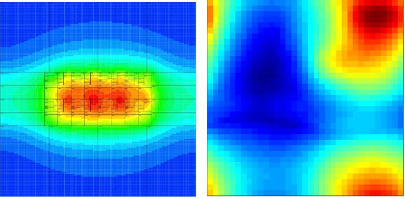
Although thermal gradient-aware k-means clustering works well under many condi-tions, this technique is not always optimal in complex hot spot distribution scenarios and may produce solutions worse than the basic k-means approach. Hot spots are often sorted into inappropriate clusters due to their common temperature and regardless of their physical locations on the chip. Figures 3.2(a) and 3.2(b) show k-means clustering results using basic and thermal-gradient aware on the same set of hot spot points with eight sensors. Although the clustering of hot spots varies slightly for the two methods, the sensor placement loca-tions are almost identical. To make a difference in sensor placement, the temperatures of the hot spots used in thermal gradient-aware k-means calculations can be scaled according to Equation 3.4, whereais a constant specifying the steepness of the temperature gradient.

New T emperatures=a· Original T emperatures

Maximum T emperature (3.4)

Figures 3.2(c) and 3.2(d) show the clustering results of using Equation 3.4 with a = 1000 and a = 2500, respectively, on the same hot spot set used in Figures 3.2(a) and 3.2(b). In both situations, the sensors have been placed closer to the hot spots of higher temperature and further from the hot spots of lower temperature. Many of the hot spot cluster assignments, however, are not appropriate spatially. In Figure 3.2(d), for example, many of the red hot spots clustered with sensor S1 would be more appropriately grouped with the gray hot spots clustered with sensor S2, and vice versa.

(a) Basic K-means (b) Thermal-Aware K-means, a = 1

(c) Thermal-Aware K-means, a = 1000 (d) Thermal-Aware K-means, a = 2500

Figure 3.2: K-means clustering sensor placement variations.

3.2.3 Hot Spot Determination in Regard to Sensor Allocation

There are many properties to consider when determining which locations on the chip are considered to be ”hot spots.” Varying the determination rules has the potential to signifi-cantly affect the resulting sensor placement locations. The trade-offs between full thermal map characterization and hot spot detection must be considered when identifying initial hot spot locations.

Local Hot Spots

encourages sensor placement across the entire die and is most appropriate for characterizing the full thermal map of the processor. The hot spot locations will be the points that reach the local maximum temperature for each functional block. For many functional blocks, the hottest points will be the near the edges of the block adjacent to a hotter component.

Global Hot Spots

A second method of hot spot determination is to record global hot spots, or any location on the die that reaches or surpasses a specified emergency temperature threshold, typically near82◦_{C or 355K[41][44]. Temperature sensors will be placed closer to the locations on} the chip of significantly higher temperature, and thus will not likely be spread across the chip. This technique is best for quickly recognizing emergency temperatures as opposed to recovering the full thermal map of the entire processor. Furthermore, the number of hot spots determined by this technique is inversely correlated with the specified emergency temperature threshold. A higher threshold will result in fewer hot spots that could all be located within a single functional block in the processor. Alternatively, a low enough threshold will result in many hot spots, which could potentially cover more than 50% of the processor. A large number of hot spots would allow sensors to be spread through a larger area. As reported in [64], the integer register file is repeatedly the hottest component in the Alpha 21364 core across the SPEC2000 benchmarks. Choosing a high emergency temperature threshold could result in placing sensors only in the integer register file, while a lower threshold would allow sensors to be placed in adjacent functional blocks across the processor. The tradeoffs between quick hot spot detection and full thermal map recovery must be considered.

3.3 Non-Uniform Subsampling of Thermal Maps

are not very effective in placing sensors near the hottest points. To reduce the number of points to be clustered while maintaining clear representation of thermal data, non-uniform subsampling algorithms can be used obtain a subset of key thermal analysis locations on a chip. More samples are selected from regions of higher temperature and fewer points are selected from regions of lower temperature. Subsampling a thermal map will likely strike a balance between uniform temperature measurement and thermal emergency detection. After the thermal map has been subsampled, clustering algorithms can be used on the subsamples to determine sensor placement locations.

The two gradient based non-uniform subsampling algorithms for images proposed in [54] select sample pixels from a given image such that a constant gradient region will be represented by a number of samples linearly proportional to the gradient magnitude.

Deterministic Subsampling

The deterministic version of this algorithm states that in order to quantize the data set ||∇I1||intoQlevels, a list of pixel locations Iq with a quantized gradient norm ofq must

be built for each levelq. After all pixels have been distributed into appropriate quantization levels,every sqth pixel in each list Iq will be selected, where sq = dc/qe for a constant c. This specification ensures that samples are selected more frequently in regions of high gradient. The constant valuecis adjusted to yield a larger or smaller number of samples.

Applying subsampling algorithms to a full thermal map of a processor core while treat-ing the temperature values as gradients results in more samples closer to the regions with more hot spots and fewer samples near cooler regions. Adjusting the value ofcaffects the number of samples taken from a thermal map. Before performing subsampling, the tem-perature should be normalized according to Equation 3.5 using the minimum temtem-perature

Tminand maximum temperatureTmax in the thermal map used for analysis.

Inorm =

||∇I1|| −Tmin Tmax−Tmin

(3.5)

map yielded the sampled results displayed in Figure 3.3(a) and 3.3(b). Both runs used 25 quantization levels. Figure 3.3(a) shows the results from setting the constantc = 5. This constant produced many fewer samples than setting the constant c = 0.25 as shown in Figure 3.3(b). Both plots reveal sampling locations spread throughout the entire thermal map. This algorithm is fairly conservative and similar to uniform sampling.

(a) Thermal deterministic subsamples from

c= 5

(b) Thermal deterministic subsamples fromc= 0.25

Figure 3.3: Thermal deterministic non-uniform subsampling results with 25 quantization levels.

Stochastic Subsampling

A stochastic version of non-uniform sampling looks at each individual pixel location(i, j) and decides whether to select this pixel as a sample or not. Pixels are selected with prob-abilityp(i, j) = min(α∗ ||∇I1||(i, j),1). Adjusting the proportionality constantα yields

fewer or additional samples.

Performing the stochastic non-uniform subsampling algorithm on a sample thermal map yielded the sampled results displayed in Figure 3.4. Figure 3.4(a) shows the results from setting the constantα = 1.5, which produced fewer samples than setting the constant

regions, and only one or two samples in the coolest region. The samples taken in this stochastic subsampling algorithm accurately reflect the thermal gradient of the chip.

(a) Thermal stochastic subsamples fromα = 1.5

(b) Thermal stochastic subsamples fromα= 5

Figure 3.4: Thermal stochastic non-uniform subsampling results.

Chapter 4

Simulation Framework

4.1 Multi-Core Architectures

Due to their improved performance per watt efficiency [50], multi-core processors have become the new industry standard, packing more cores onto a single die with each gen-eration [5][31]. Positioning of the cores within a processor floorplan affects the thermal distribution and maximum temperatures. Two common layouts are displayed in Figure 4.1 for 8-core architectures. Recent trends indicate that the dense floorplan with cores placed immediately next to each other in Figure 4.1(a) is more popular in modern-day many-core processors [5] [50]. The sparse floorplan in Figure 4.1(b) has been used to prevent thermal coupling between the cores [36]. Both floorplan options were analyzed in this thesis.

4.2 Simulation Platform

(a) Dense 8-core architecture. (b) Sparse 8-core architecture.

Figure 4.1: 8-Core architecture floorplans used in simulation.

Alpha 21364 Parameters

Level 1 instruction and data caches 4-way associative

64 KB with 32-byte block size 2 cycle latency.

Level 2 cache Unified 4-way associative 512 KB with 128-byte line size 15 cycle latency

Load store queue 32 Register update unit 64 Nominal Frequency 3 GHz

NominalVdd 1.3 V

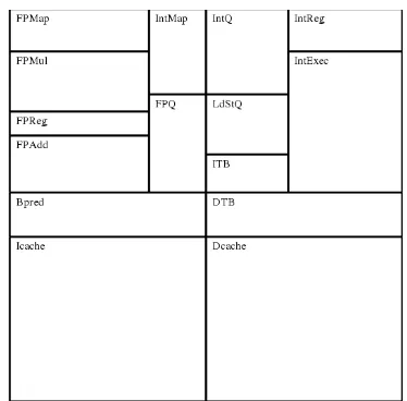
Figure 4.2: Alpha 21364 core architecture.

The SPEC2000 benchmark suite [66] was simulated using SimpleScalar Version 2.0 [11]. SimpleScalar is a well-known cycle-by-cycle functional microarchitectural simulator. The version of SimpleScalar used in this thesis was configured to more accurately model the inner workings of the Alpha 21364 processor. A microarchitectural-level power analysis tool, Wattch [10], was integrated with SimpleScalar to obtain realistic dynamic power trace data every 10,000 cycles for the 21364. Leakage power was modeled as a percentage of each functional block’s dynamic power. Additional leakage power resulting from high temperatures was provided in thermal simulations.

4.3 Modifications to the HotSpot Framework

To ensure that power trace data from Wattch has been scaled appropriately for the chosen technology sizes in these experiments, Equation 4.1 was used in conjunction with tech-nology trend data from the International Techtech-nology Roadmap for Semiconductors [59] and Dennard scaling [17]. The equation for dynamic power,Pdynamic, reveals that average

device capacitance and operating frequency scale linearly with power, whileVddis squared.

Pdynamic = 0.5αCVdd2f (4.1)

Operating frequency has not scaled linearly with technology. ITRS reports a 1.73 fac-tor increase in operating frequency from 3 GHz in the 21364 to 5.2 GHz in 2005 90 nm technology. A further increase by a factor of 1.128 to 5.87 GHz in 45 nm 2010 technology was reported by ITRS. Together, these factors bring a total of a 1.95 scaling factor from 130 nm technology. Dennard scaling reports that average device capacitance has scaled linearly by factor of 0.7. Recent ITRS trends show that this linear increase has slowed to a factor of 0.55 since 2005. Combining these factors gives a total capacitance scaling factor of 0.3885. The 130 nm 21364 was implemented withVdd = 1.3V. ITRS reported that at 45

nm technology in 2010,Vdd= 0.97V. This gives aVdd scaling factor of0.7692. Combining

all scaling factors together gives a total dynamic power scaling factor from 130 nm to 45 nm of 0.38.

To ensure that a realistic heat sink and spreader were modeled appropriately for a scaled architecture, both the physical size and the average expected power Pavg of each die were

taken into account. The chosen spreader size was set to twice the size of the die and the sink was set to four times the size of the die. These sizing ratios were chosen in accor-dance with similar research done in [41] and to mimic various modern processors [27][53]. Heat sink convection resistance was calculated according to Equation 4.2 using an average temperatureTavg of 333K and ambient temperatureTamb of 318K. This equation ensures

specified average power. Using these specifications, the sink and spreader parameters were chosen as shown in Table 4.2 for the architectures used in the following experiments.

Convection resistance= Tavg−Tamb

Pavg

(4.2)

Component Scaled Size

Die size 0.015 m Spreader size 0.031 m Sink size 0.062 m Convection resistance 0.1645 (K/W)

Table 4.2: Sink and spreader sizes used in HotSpot simulation for the 8-core architectures.

Additional HotSpot configuration modifications included the thickness of the sink, spreader, die, and thermal interface material. These parameters were set to the same values presented in [41] and are displayed in Table 4.3. All other parameters were left as the de-fault HotSpot values. To reflect realistic sensing capabilities, all sensors are assumed to be accurate within 2K of the true thermal data.

Parameter Value

Spreader thickness 0.1 cm Sink thickness 0.7 cm Die thickness 0.05 cm Thermal interface material thickness 0.0075 cm

Table 4.3: Default HotSpot configuration modifications.

4.4 Representative Benchmarks

The SPEC2000 benchmarks were used in this thesis. The work in [64] addresses the power and thermal characteristics of the SPEC2000 benchmarks on the Alpha 21364. A represen-tative set of 11 of the 26 available benchmarks were presented. A summary of the chosen benchmarks is displayed in Table 4.4. Each of these benchmarks was run through an in-tegrated version of SimpleScalar/Wattch to obtain detailed power trace data for the single core 21364. Each benchmark was fast-forwarded to a representative sample of 500 million instructions and run through HotSpot twice. The first run was used to represent warm-up of all components and input as initial temperature for the second run. Temperature results from the second run were used in all further analysis.

IPC Average % Cycles in Dynamic Steady Sink

Power Thermal Max State Temp

(W) Violation Temp (◦_{C) Temp (}◦_{C) (}◦_C)

Low Thermal Stress (cold)

parser(I) 1.8 27.2 0.0 79.0 77.8 66.8

facerec(F) 2.5 29.0 0.0 80.6 79.0 68.3

Severe Thermal Stress (medium)

mesa(F) 2.7 31.5 40.6 83.4 82.6 70.3

perlbmk(I) 2.3 30.4 31.1 83.5 81.6 69.4

gzip(I) 2.3 31.0 66.9 84.0 83.1 69.8

bzip2(I) 2.3 31.7 67.1 86.3 83.3 70.4

Extreme Thermal Stress (hot)

eon(I) 2.3 33.2 100.0 84.1 84.0 71.6

crafty(I) 2.5 31.8 100.0 84.1 84.1 70.5

vortex(I) 2.6 32.1 100.0 84.5 84.4 70.8

gcc(I) 2.2 32.2 100.0 85.5 84.5 70.8

art(F) 2.4 38.1 100.0 87.3 87.1 75.5

Table 4.4: Thermal information for the SPEC2000 benchmarks, generated in [64].

equal to 82◦_{C. For the simulations in this thesis, benchmarks were chosen based on the} listed thermal characteristics and thermal stress categories.

To simulate multi-core processors, power trace data specific to each benchmark was replicated, scaled appropriately, and assigned to individual cores in the multi-core config-urations in various combinations. As done in [64], each benchmark was fast-forwarded to a representative sample of 500 million instructions and run through HotSpot twice, using the first run to represent warm-up and as an input as initial temperature for the second run. Temperature results from the second run were used in all further analysis in this thesis. The benchmarks chosen for simulation of the 8-core architectures are displayed in Table 4.5, where each core represents those labeled previously in Figures 4.1(a) and 4.1(b). The first set contains benchmarks all from the Extreme Thermal Stress category, and the second contains a mix of benchmarks from all three categories. These two test sets offer a variety of interesting thermal patterns for analysis.

Core Set 1: Hot Benchmarks Set 2: Mix of Benchmarks

C0 art parser

C1 gcc art

C2 vortex bzip2

C3 eon bzip2

C4 eon parser

C5 vortex art

C6 gcc gcc

C7 art bzip2

Chapter 5

Analysis of Thermal Sensor Placement

Mechanisms

To determine sensor placement, the benchmark with the highest average power and hottest average temperatures,art, was applied to every core in each architecture. HotSpot simula-tions were conducted with this benchmark configuration to determine the common hot spot locations. The hottest temperatures encountered for every location on the chip throughout the simulation were recorded. Maximum temperatures for all eight cores were folded onto a single core to obtain a thermal map of all maximum temperatures seen on a core. A ther-mal gradient map of the resulting temperatures is shown in Figure 5. The hottest functional block for the sparse architecture was the data cache.

Hot spot locations were determined from this thermal map. For the standard k-means clustering simulations used in this thesis, any location on the chip that has recorded a temperature of 82◦_{C or higher at any time is considered a hot spot, while the non-uniform} subsampling simulations analyzed the entire thermal map before clustering.

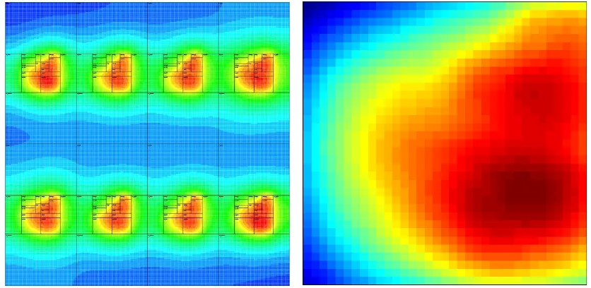
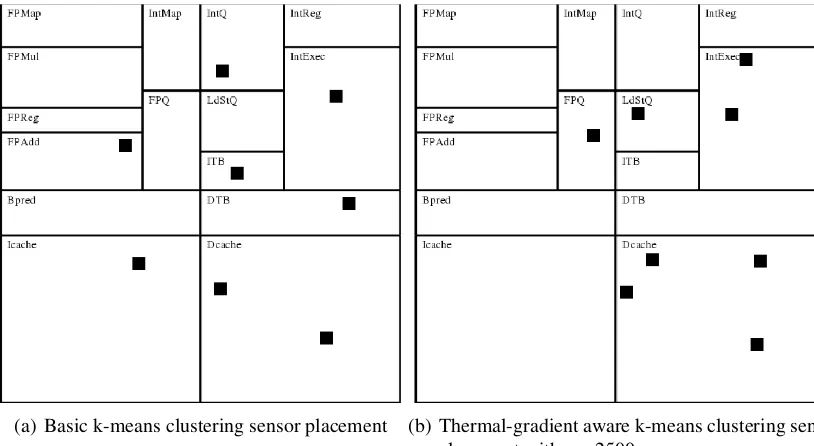
The basic k-means clustering algorithm was implemented on the folded maximum tem-peratures core from the 8-core sparse architecture for eight thermal sensors. This algorithm resulted in the sensor placement displayed in Figure 5.2(a). Six of the eight sensors were placed in the right-side of the core, while the remaining two were spread out evenly into the FPAdd and I-cache.

(a) 8-Core sparse architecture maximum tempera-tures folded onto a single chip

(b) Maximum core temperatures from the 8-core sparse architecture folded onto a single core

Figure 5.1: Thermal maps of the 8-core sparse architecture maximum temperatures.

same folded maximum temperatures core. This algorithm placed four sensors in the D-cache, two in the IntExec, and two in the load-store queue and floating-point queue. The remaining functional blocks were left without any nearby thermal sensors.

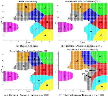
The stochastic non-uniform subsampling algorithm was used on the same core thermal map to produce the sampling locations shown in Figure 5.3(a). These samples were then clustered using the basic k-means approach, producing the sensor locations displayed in Figure 5.3(b). Three sensors were placed in the D-cache, the hottest unit. The remaining five sensors were placed in the Icache, FPReg, IntQ, integer register file, and IntExec. Though these five sensors were not necessarily placed near areas of significant temperature, they were placed throughout the core to accurately represent the thermal gradient.

(a) Basic k-means clustering sensor placement (b) Thermal-gradient aware k-means clustering sen-sor placement with a = 2500

Figure 5.2: Sensor placement using k-means clustering on a single core in the 8-core sparse architecture.

(a) Samples taken using stochastic non-uniform subsampling

(b) Sensor placement via basic k-means clustering of sample points

temperatures for all cores in each architecture. Maximum error refers to the largest er-ror in estimated temperature observed in a core for each sensor configuration. Both linear and cubic interpolation were used in temperature estimation between the sensors. Positive temperature errors indicate that the sensor placement and reconstruction scheme combina-tion resulted in overestimated temperatures, while negative temperature errors indicate an underestimate.

The thermal-gradient aware k-means clustering sensor placement had an improvement in all errors over basic k-means clustering sensor placement for the sparse architecture. Non-uniform subsampling showed the lowest average error and lowest maximum error for both test sets and both interpolation methods. All three sensor placement algorithms resulted in maximum errors of at least 9.09◦_{C overestimate. These overestimates were} observed in the cooler regions of each core. No overestimates were high enough to be considered a false thermal emergency (greater than or equal to 82◦_C).

Sensor Placement _{Test Set} Interpolation Mean Maximum _Improvement

Method Method Error Error

Basic K-means

Set 1 Linear 1.29◦_{C 14.86}◦_C -Set 2 Linear 1.44◦_{C 13.75}◦_C

-Set 1 Cubic 1.38◦_{C 15.7}◦_C

-Set 2 Cubic 1.84◦_{C 13.75}◦_C

- Thermal-Gradient Aware K-means

Set 1 Linear 1.02◦_{C 13.51}◦_{C 20%} Set 2 Linear 1.16◦_{C 14.04}◦_{C 19%} Set 1 Cubic 0.98◦_{C 14.36}◦_{C 28%} Set 2 Cubic 1.17◦_{C 13.59}◦_{C 35%}

Non-Uniform Subsampling

Set 1 Linear -0.31◦_{C 9.09}◦_{C 76%} Set 2 Linear -0.29◦_{C 10.16}◦_{C 79%} Set 1 Cubic -0.17◦_{C 9.24}◦_{C 88%} Set 2 Cubic -0.18◦_{C 9.55}◦_{C 90%}

Table 5.1: 8-Core sparse architecture thermal reconstruction results, with minimum errors in boldface text.

single core. A thermal gradient map of the resulting temperatures is shown in Figure 5. The hottest functional block for the dense architecture was the integer register file. The lateral heat propagation from this functional block created significant temperatures in other functional blocks in adjacent cores.

(a) 8-Core dense architecture maximum tempera-tures folded onto a single chip

(b) Maximum core temperatures from the 8-core dense architecture folded onto a single core

Figure 5.4: Thermal maps of the 8-core sparse architecture maximum temperatures.

The basic k-means clustering algorithm was implemented on the folded maximum tem-peratures core from the 8-core dense architecture for eight thermal sensors. This algorithm resulted in the sensor placement displayed in Figure 5.5(a). Four of the eight sensors were placed in the upper right corner near the integer functional blocks. The other sensors cov-ered the remaining corners of the core, leaving the center of the core without any sensors.

The thermal-gradient aware k-means clustering algorithm was also implemented on the same folded maximum temperatures core. this algorithm placed five sensors near the integer functional blocks. Two sensors were placed in the bottom of the D-cache and one sensor was placed in the FPMap. The hot spots in the I-cache were left without nearby sensors.

(a) Basic k-means clustering sensor placement (b) Thermal-gradient aware k-means clustering sen-sor placement with a = 2500

Figure 5.5: Sensor placement using k-means clustering on a single core in the 8-core dense architecture.

map from the dense architecture to produce the sampling locations displayed in Figure 5.6(a). These samples were then clustered using the basic k-means approach, producing the sensor locations shown in Figure 5.6(b). Three sensors were placed in the integer functional blocks, the hottest units in the core. Two sensors were placed in the D-cache, another considerably hot functional block. Three of the remaining sensors were placed in the other two corners of the core, covering the lateral heat propagation from the integer register file in adjacent cores. A single sensor was placed near the center of the core to measure the expected cooler temperatures.

(a) Samples taken using stochastic non-uniform subsampling

(b) Sensor placement via basic k-means clustering of sample points

Figure 5.6: Non-uniform subsampling with k-means clustering sensor placement on a sin-gle core in the 8-core dense architecture.

The thermal-gradient aware k-means clustering sensor placement on the dense archi-tecture had a much greater mean error and maximum error for both test sets and both interpolation methods, while both basic k-means clustering and non-uniform subsampling errors noticeably improved for the dense architecture over the sparse architecture.

The thermal-gradient aware k-means clustering results are consistent with those en-countered in [41]. This algorithm was more successful in the sparse architecture because each core is thermally insulated with the L2-cache. The thermal patterns within each core were very similar, unlike the core patterns in the dense architecture. In the dense architec-ture, the cores thermally influence each other much more easily. Using a sensor placement mechanism that places sensors only near hot spots is not as effective for dense architectures because not all cores will have similar hot spots. A more conservative sensor placement mechanism, such as non-uniform subsampling, is better suited for a dense architecture.

Sensor Placement

Test Set Interpolation Mean Maximum Improvement

Method Method Error Error

Basic K-means

Set 1 Linear -0.52◦_{C 3.8}◦_C -Set 2 Linear -0.50◦_{C 3.81}◦_C -Set 1 Cubic -0.34◦_{C 3.13}◦_C

-Set 2 Cubic 0.38◦_{C 3.18}◦_C

- Thermal-Gradient Aware K-means

Set 1 Linear -2.58◦_{C -9.20}◦_C -Set 2 Linear -2.98◦_{C -10.74}◦_C -Set 1 Cubic -2.46-◦_{C -11.02}◦_C -Set 2 Cubic -2.90◦_{C -8.15}◦_C

-Non-Uniform Subsampling

Set 1 Linear -0.07◦_{C -3.41}◦_{C 86%} Set 2 Linear -0.06◦_{C -3.42}◦_{C 88%} Set 1 Cubic 0.05◦_{C -2.94}◦_{C 85%} Set 2 Cubic 0.04◦_{C -2.96}◦_{C 89%}

Table 5.2: 8-Core dense architecture thermal reconstruction results, with minimum errors in boldface text.

Chapter 6

Sensor Mini-Network

Sensor networks on chip for the purpose of thermal monitoring have not been researched extensively in the past. The work in [70] focuses on network interfaces and routing in a Monitor Network on a Chip (MNoC) architecture for multi-core processor. This work does not focus on improving thermal map data recovery, but on data collection, network latency minimization, and area cost reduction.

Use of an MNoC architecture has been proposed for multi-core processor thermal mon-itoring in [69] with focus on thermal sensor placement. Two different approaches were analyzed:

• Regular MNoC structureModify the basic k-means clustering algorithm to treat the MNoC interfaces as special hotspots with fixed locations for the purpose of reducing wire length and therefore latency.

• Flexible MNoC structureExecute sensor placement without concern of the MNoC interfaces. Subsequently cluster the sensors using the basic k-means clustering ap-proach and place the MNoC interfaces at the centroid of each cluster.

6.1 Sensor Mini-Network Configuration

temperature-related reliability concerns, thus maximum thermal coverage with a minimal number of sensors is of utmost importance. Using a large number of sensors for coverage of a single core is too complicated for kilocore systems and will incur excessive overheads in terms of area and power. For this reason, a minimum number of thermal sensors will be placed on each core at points that are most beneficial for capturing the core’s thermal activity at run-time.

The sensors will be arranged in a Sensor Mini-Network (SMN) for the purpose of sens-ing the complete thermal profile of a chip. A 64-homogeneous core version of the SMN is depicted in Figure 6.1. Each sensor periodically reports its measured temperature to a Reliability Unit so that it can be used in conjunction with temperatures from other sensors to ultimately determine thermal information for locations on the chip that are not directly measured by the sensors. The SMN configuration is more accurately able to sense thermal violations across the entire chip than the same number of sensors using no communication.

To determine the appropriate number of bits required to encode all temperature data sufficiently, the minimum and maximum expected temperatures for a specific architec-ture must be considered according to Equation 6.1. The difference between the maximum temperature Tmax and the minimum temperatureTmin (set to the ambient temperature) is

divided by the desired resolution in Kelvin. This calculation give the necessary number of codes to be used, from which the required number of bits,n, can be calculated.

Number of codes= Tmax−Tmin

Resolution (6.1)

For the following discussions, consider a 1024-core architecture modeled at 25 nm technology. A representative trace of typical thermal operation was obtained for each of the 1024 cores running a randomly selected benchmark from Table 4.4. Thermal simulations were conducted using HotSpot 5.0 at a grid size of 1024 x 1024. The corresponding thermal map is displayed in Figure 6.2. A uniform grid of sensors placed evenly across the die is assumed for simplicity. Histograms of the temperatures seen at these sensor locations are shown in Figures 6.3(a) and 6.3(b) for a total of 2048 thermal sensors (Configuration A) and a second scenario of 1024 sensors (Configuration B). These histograms indicate all possible expected temperature measurements that will need to be represented in the SMN. For both configurations in the 1024-core architecture, all observed temperatures were under 400K.

Figure 6.2: Steady-state thermal map of a homogeneous 1024-core architecture.

3300 340 350 360 370 380 390 400 20

40 60 80 100 120 140

Sensor Temperature in Kelvin

(a) Accumulated sensor readings from using 2048 sensors (Configuration A).

3400 350 360 370 380 390 400 5

10 15 20 25 30 35 40

Sensor Temperature in Kelvin

(b) Accumulated sensor readings from using 1024 sensors (Configuration B).

−1.50 −1 −0.5 0 0.5 1 1.5 2 2.5 3 2 4 6 8 10 12 14x 10

4

Error in Degrees Kelvin

(a) Error in estimation from using 2048 Sensors (Configuration A).

−60 −5 −4 −3 −2 −1 0 1 2 1 2 3 4 5 6 7x 10

4

Error in Degrees Kelvin

(b) Error in estimation from using 1024 Sensors (Configuration B).

Figure 6.4: Magnitudes of all temperature estimation errors for the 1024-core architecture.

6.1.1 Baseline SMN [No Compression]

The most straight-forward SMN configuration is to have each thermal sensor report its temperature individually to the Reliability Unit without compressing any data. There is no communication between sensors; all sensors are handled identically. Linear interpolation between the sensors is used to determine the thermal data for the entire chip, similar to the interpolation-based uniform strategy discussed previously.

Temperature Range 7-bit Code Q-level Quantized Temperature

317.5Kto 318.5K 000 0000 Q0 318

318.5Kto 319.5K 000 0001 Q1 319

319.5Kto 320.5K 000 0010 Q2 320

· · · ·

· · · ·

· · · ·

443.5Kto 444.5K 111 1111 Q127 444

Table 6.1: Temperature quantization levels for the 1024-core architecture.

6.1.2 SMN Differential Encoding

To reduce communication bandwidth and overall power consumption, the amount of trans-mitted data should be minimized. In the differential encoding algorithm, some sensors are assigned to be reference sensors and the remaining are node sensors. Assuming that ther-mal sensors have been uniformly placed in a grid throughout the die, every-other sensor will be a reference sensor. A sample setup of nine sensors is shown in Figure 6.5. Sensors

S0, S2, S6,andS8are references sensors whileS1, S3, S4, S5,andS7are node sensors.

Figure 6.5: Uniform grid of reference and node sensors.

The SMN differential encoding setup is displayed in Figure 6.6. The reference sensors sample and digitize their uncompressed temperature Tref erence and send the result to the

uncompressed 7-bit temperature representation as displayed in Table 6.1. The reference sensors located closest to each node sensor can be used to reduce the number of bits needed to represent the temperature at each node sensor. Each node sensor is assumed to be able to receive the two closest located reference sensors’ uncompressed transmissions. From these two transmissions, an estimate temperature for the node sensor is computed using basic linear interpolation. The difference between this estimate and the node sensor’s true temperatureTnodeis computed, compressed, and transmitted to the Reliability Unit.

The node sensor temperature represented as a compressed codeword will be sent to the Reliability Unit where it will be decoded into a temperature difference. This decoded difference will subsequently be added to the temperature estimate from the corresponding reference sensors in order to recover the true temperature for this node sensor.

Figure 6.6: SMN differential encoding block diagram.

To determine the fewest possible number of bits required for the node sensor code-words at the specified resolution, statistical data for the given architecture must be gathered surrounding the accuracies of linearly estimating solely using reference sensors.

distance from their corresponding reference sensors. Histograms of the errors for the 1024-core architecture using 1024 reference sensors and 512 reference sensors are shown in Figures 6.7(a) and 6.7(b).

(a) Temperature estimation error for Configuration A, 1024 Reference Sensors.

(b) Temperature estimation error for Configuration B, 512 Reference Sensors.

Figure 6.7: Temperature estimation error histograms at node sensor locations in the 1024-core architecture

The mean of the gathered errors should be equal to zero. To ensure that this is the case, the temperature estimation T can be offset by the true mean according to Equation 6.2, wheree¯(x, y)is equal to the true mean of the error at a distance(x, y)from the reference sensors. Using this equation with the original histograms from Figures 6.7(a) and 6.7(b) generates the updated histograms in Figures 6.8(a) and 6.8(b).

ˆ

T(x, y) =α(x, y)T(x1, y1) +β(x, y)T(x2, y2) + ¯e(x, y) (6.2)

Gathering the errors in estimation for all node sensor locations yields a fixed range of possible estimation errors. This range divided by the desired resolution gives the num-ber of codewords required and the necessary numnum-ber of bits via Equation 6.1. All node sensor temperatures will be encoded into these compressed codewords. Several different quantization temperature levels are assigned to the same codeword.

(a) Temperature estimation error with adjusted mean for Configuration A, 1024 Reference Sensors.

(b) Temperature estimation error with adjusted mean for Configuration B, 512 Reference Sensors.

Figure 6.8: Temperature estimation error histograms with adjusted mean at node sensor locations in the 1024-core architecture

sensors and 512 node sensors, Figure 6.8(b) shows that a minimum of seven codewords are needed at the same resolution, which can be represented in a minimum of three bits. Tables 6.2 and 6.3 display a more detailed summary of codeword assignments for these two scenarios.

Temperature Difference Range 2-bit Codeword

-1.5K to -0.5K 00 =C0

-0.5K to 0.5K 01 =C1

0.5K to 1.5K 10 =C2

1.5K to 2.5K 11 =C3

Table 6.2: 2-Bit codewords for SMN differential encoding compression in the 1024-core architecture.

Temperature Difference Range 3-bit Codeword

-4.5K to -3.5K 000 =C0

-3.5K to -2.5K 001 =C1

-2.5K to -1.5K 010 =C2

-1.5K to -0.5K 011 =C3

-0.5K to 0.5K 100 =C4

0.5K to 1.5K 101 =C5

1.5K to 2.5K 110 =C6

2.5K to 3.5K 111 =C7

Table 6.3: 3-Bit codewords for SMN differential encoding compression in the 1024-core architecture.

Scheme Reference Node Bits Transmitted Max Improvement

Sensors Sensors to Reliability Unit Error

No compression 2048 0 14,336 3K

-2-bit Diff. Encoding 1024 1024 11,980 3K 36%

No compression 1024 0 7,168 6K

-3-bit Diff. Encoding 512 512 5,120 6K 29%

Table 6.4: SMN differential encoding performance results.

fewer bits for compressed codewords to achieve a further improvement in performance at the cost of more erroneous decoding. Both configurations in this example were assigned codeword sizes to account for the full histogram of error possibilities, however, an unfore-seen outlying temperature difference could occur and cause incorrect temperature recovery. This trade-off must be considered when designing the SMN with differential encoding.

Though the number of transmitted bits to the Reliability Unit is significantly reduced through differential encoding, additional power is required for the reference sensor tem-peratures to reach the node sensors. To eliminate this cost and reduce routing complexity, compression through distributed source coding was explored.

6.1.3 SMN Distributed Source Coding

A second method of compressing the temperature data and reducing the number of bits to transmit can be achieved by using counters and eliminating communication between the reference and node sensors. The node sensor temperatures can still be compressed without losing any vital thermal information at their locations. The reference sensors send uncom-pressed data to the Reliability Unit while the node sensors are comuncom-pressed using distributed source coding (DSC). Figure 6.9 shows a block diagram of SMN with DSC for two ref-erence senors and one node sensor. Each sensor sends its compressed or uncompressed temperature directly to the Reliability Unit where the compressed node temperaturesTnode

are decoded into original temperatures.

Figure 6.9: SMN distributed source coding block diagram.

the counter will be stopped and its current output value will be recorded as the encoded temperature for that sensor. To reduce the number of bits required, the reference sensor will use an n-bit counter and n bits to represent the transmitted reference temperature,

Tref erence. Each node sensor uses m fewer bits to represent the temperature. The node

sensors use a smaller n − m-bit counter and an n − m-bit codeword to represent their transmitted temperature.

Figure 6.10: SMN distributed source coding sensor counters.

To determine the fewest possible number of bits required for node sensor codeword at the specified resolution, statistical data for the given architecture must be gathered sur-rounding the accuracies of linearly estimating solely using reference sensors, as done in SMN differential encoding. The same process of determining the maximum error in tem-perature estimation at all node sensor locations can be used for SMN distributed source coding. The error histograms are the same in both compression schemes because use the same linear estimation from the same thermal trace data.

(Configuration A), it can be deduced from the SMN differential encoding codeword size determination process that a minimum of four codewords are needed at a resolution of 1K, which can be represented in two bits. For the scenario with 512 reference sensors and 512 node sensors (Configuration B), Figure 6.8(b) shows that a minimum of seven codewords are needed at the same resolution, which can be represented in a minimum of three bits. In SMN, these codewords represent the actual temperature measured by the node sensors, rather than the difference between the estimate and the true temperature. Table 6.5 displays a more detailed summary of codeword assignments and representations for these two sce-narios. The Q-levels correspond to the same 7-bit representations displayed previously in Figure 6.1.

Temperature Range 2-bit 3-bit Q-level Quantized

Codeword Codeword Temperature

317.5Kto 318.5K 00 =C0 000 =C0 Q0 318

318.5Kto 319.5K 01 =C1 001 =C1 Q1 319 319.5Kto 320.5K 10 =C2 010 =C2 Q2 320

320.5Kto 321.5K 11 =C3 011 =C3 Q3 321

321.5Kto 322.5K 00 =C0 100 =C4 Q4 322 322.5Kto 323.5K 01 =C1 101 =C5 Q5 323

323.5Kto 324.5K 10 =C2 110 =C6 Q6 324

324.5Kto 325.5K 11 =C3 111 =C7 Q7 325 325.5Kto 326.5K 00 =C0 000 =C0 Q8 326

326.5Kto 327.5K 01 =C1 001 =C1 Q9 327

· · · · ·

· · · · ·

· · · · ·

443.5Kto 444.5K 11 =C3 111 =C7 Q127 444

Table 6.5: Codewords for SMN distributed source compression in the 1024-core architec-ture.

Figure 6.11 illustrates an example of this comparison process for the 1024-core ar-chitecture with 1024 reference sensors at 1024 node sensors represented with 2-bit error codewords (Configuration A). A node sensor measures 342.6 K, which falls in the range 342.5K to 343.5Kand is represented with codewordC1. The node sensor sendsC1to the

Reliability Unit where it is compared with the estimate for this location. In this case, the estimate is 341K, which is represented with the quantization levelQ23. A histogram of the

possible error in the estimate is super-imposed over this quantization level, centering the zero-point overQ23. The closest quantization levels toQ23that correspond to a codeword

ofC1 areQ21 andQ25. Because the error histogram centered at estimateQ23overlaps the

ambiguous code Q25 and not Q21, the recovered node sensor temperature is quantization

levelQ25, or 343K.

Table 6.6 displays the performance results for the 1024-core architecture using both sensor configuration scenarios. Using DSC to compress node sensor temperatures in both sensor configurations significantly improves the number of transmitted bits to the Reliabil-ity Unit over a no compression scenario without losing any information.

Scheme Reference Node Bits Transmitted Max Improvement

Sensors Sensors to Reliability Unit Error

No compression 2048 0 14,336 3K

-2-bit DSC 1024 1024 11,980 3K 36%

No compression 1024 0 7,168 6K

-3-bit DSC 512 512 5,120 6K 29%

Table 6.6: SMN distributed source coding performance results.

(as compared to the no compression scheme) to encode the node sensor codewords. Com-paring overheads of the Reliability Unit is beyond the scope of this thesis.

6.2 SMN on a 1024-Core Architecture

The previously discussed compression schemes within an SMN could also be applied to architectures containing many sensors for each core. Consider the 1024-core architecture from Section 6.1 with nine sensors for each core, arranged in a uniform grid. Increasing the number of sensors reflects a more realistic scenario where each core has multiple sensors. The temperatures measured by these sensors are accumulated in Figure 6.12(a). The mag-nitudes of all errors in temperature estimation through linear interpolation are accumulated in the histogram in Figure 6.12(b). Measuring temperature in the 1024-core architecture was much more accurate with this number of sensors; 95% of the errors were under 0.4K

and 100% of the observed errors were under 1K.

(a) All measured temperatures in the 1024-core ar-chitecture using 9 sensors per core.

(b) Error in estimation from using 9 sensor for every core.

Figure 6.12: Magnitudes of all temperature estimation errors for the 1024-core architecture.

As seen in the previous sensor configurations of 1024 sensors and 2048 sensors, all observed measured temperatures were under 400 K. The ambient temperature for the ex-periment was still set to 318 K, so this sensor configuration will use the same 7-bit code representation previously displayed in Table 6.1.

node sensors will be used for each core. To compress the node sensor temperatures, the temperature estimation error histogram for each node sensor location in Figure 6.13(a) and its adjusted mean histogram in Figure 6.13(b) reveal a maximum expected error of 0.5K. If a resolution of 1Kis specified, then a maximum of one bit is needed for each node sensor. Tables 6.7 and 6.8 display the temperature error range assignments for this configuration.

(a) Temperature estimation error for the node sen-sors.

(b) Temperature estimation error with adjusted mean for the node sensors.

Figure 6.13: Temperature estimation error histograms at node sensor locations in the 1024-core architecture

Temperature Difference Range 1-bit Codeword

-0.5K to 0.5K 0 =C0

0.5K to 1.0K 1 =C1

Table 6.7: 1-Bit codewords for SMN differential encoding node sensor compression in the 1024-core architecture.

Table 6.9 displays the performance results from using nine sensors per core. Using compressed codewords significantly improves the number of transmitted bits to the Relia-bility Unit over a no compression scenario without losing a