coloring problem
.
White Rose Research Online URL for this paper:
http://eprints.whiterose.ac.uk/150551/
Version: Accepted Version
Proceedings Paper:
Bossek, J. and Sudholt, D. orcid.org/0000-0001-6020-1646 (2019) Time complexity
analysis of RLS and (1 + 1) EA for the edge coloring problem. In: FOGA '19- Proceedings
of the 15th ACM/SIGEVO Conference on Foundations of Genetic Algorithms. 15th
ACM/SIGEVO Conference on Foundations of Genetic Algorithms, 27-29 Aug 2019,
Potsdam, Germany. ACM Digital Library . ISBN 9781450362542
https://doi.org/10.1145/3299904.3340311
© 2019 The Authors. This is an author-produced version of a paper subsequently
published in Proceedings of the 15th ACM/SIGEVO Conference. Uploaded in accordance
with the publisher's self-archiving policy.
[email protected]
https://eprints.whiterose.ac.uk/
Reuse
Items deposited in White Rose Research Online are protected by copyright, with all rights reserved unless
indicated otherwise. They may be downloaded and/or printed for private study, or other acts as permitted by
national copyright laws. The publisher or other rights holders may allow further reproduction and re-use of
the full text version. This is indicated by the licence information on the White Rose Research Online record
for the item.
Takedown
If you consider content in White Rose Research Online to be in breach of UK law, please notify us by
Time Complexity Analysis of RLS and (1+1) EA for the Edge
Coloring Problem
Jakob Bossek
[email protected] Dept. of Information Systems University of Münster, Münster, Germany
Dirk Sudholt
[email protected] Department of Computer Science
University of Sheield, Sheield, United Kingdom
ABSTRACT
The edge coloring problem asks for an assignment of colors to edges of a graph such that no two incident edges share the same color and the number of colors is minimized. It is known that all graphs with maximum degree∆can be colored with∆or∆+1 colors, but
it isN P-hard to determine whether∆colors are suicient. We present the irst runtime analysis of evolutionary algorithms (EAs) for the edge coloring problem. Simple EAs such as RLS and (1+1) EA eiciently ind(2∆−1)-colorings on arbitrary graphs and
optimal colorings for even and odd cycles, paths, star graphs and arbitrary trees. A partial analysis for toroids also suggests eicient runtimes in bipartite graphs with many cycles. Experiments support these indings and investigate additional graph classes such as hy-percubes, complete graphs and complete bipartite graphs. Theoret-ical and experimental results suggest that simple EAs ind optimal colorings for all these graph classes in expected timeO(∆ℓ2mlogm), wheremis the number of edges andℓis the length of the longest simple path in the graph.
CCS CONCEPTS
·Theory of computation→Theory of randomized search heuristics.
KEYWORDS
Edge coloring problem, runtime analysis
1
INTRODUCTION
Evolutionary algorithms (EAs) are general purpose, bio-inspired methods that have proven to perform extraordinarily well on a wide range of optimization problems [7]. In the last decades the-oretical analysis of EAs and related methods, especially the time complexity analysis, gained a lot of attention and came up with a manifold of analysis methods and results [2, 15, 22]. While in the beginning simple toy functions like ONEMAX were studied predominantly, research soon turned its focus to well-known com-binatorial optimization problems. So far many results are available for, e. g., minimum spanning trees [21], maximum matchings [13], shortest paths [24], Eulerian cycles [20], scheduling [28] or vertex coloring [11, 25, 26] to mention a few.
We contribute to the fundamental understanding of working principles of evolutionary algorithms by considering the edge col-oring problem. Given a simple graph withnvertices andmedges, the goal is to assign colors to the edges such that no two incident edges share the same color, called a proper coloring, and the size of
the used color palette is minimal. Edge coloring has various applica-tions in (job shop) scheduling [27] or the assignment of frequencies in iber optic networks [10].
One can easily see that each simple graph can be properly col-ored with 2∆−1 colors in timeO(∆m), where∆is the maximum
node degree in the graph. An astonishing theorem by Vizing states that any simple graph can be colored either by∆(class 1) or∆+1
(class 2) colors.1Holyer [14] proved that edge coloring isN P -hard on general graphs and hence all known exact algorithmic endeavours require exponential time. However, Misra & Gries [19] provided a constructive proof of Vizing's theorem. The resulting algorithm inds an coloring with at most∆+1 colors in timeO(nm)
and makes use of a sophisticated procedure called a fan rotation. Oftentimes, restrictions to speciic graph classes lead to more ei-cient algorithms since one can leverage structural properties. For
∆-edge-colorable bipartite graphs, algorithms with running time
O(mlogm)by Alon [1],O(∆m)by Schrijver andO(mlog∆)by Cole, Ost and Schirra [8] have been proposed.
In distributed computing many machines operate collaboratively in order to solve a problem. In the famous LOCAL communication model a network is expressed as a graphG=(V,E)with maximum degree∆where adjacent nodes perform local computations and ex-change information directly in discrete rounds via message passing (see, e. g., [18]). Here, the running time is expressed by means of the (expected) number of rounds until a given problem is solved and one usually aims for poly-logarithmic running times. Graph coloring problems (vertex and edge coloring) have a long tradition in distributed computing and have been studied extensively for decades mainly due to their symmetry breaking properties and the fact that it is easy to check solutions locally [3]. That is, to verify that a(2∆−1)-edge-coloring is proper for a certain edge one needs to check the local neighborhood only. Simple, yet eicient local randomized distributed algorithms for(2∆−1)-coloring exist for over 30 years [3]. Beating this natural barrier in the deterministic setting was a major open problem for decades. Just recently, con-siderable progress was made [4, 6, 12], e. g., by Ghafari et al. [12] who proposed a deterministic distributed algorithm that calculates a(1+o(1))∆-coloring in poly-logarithmic time in the local model as long as∆=ω(logn).
Graph coloring has been subject of studies in the context of randomized search heuristics [11, 25, 26]. This includes studies of a simple Ising model, a model of ferromagnetism where one seeks tomaximizethe number of edges where both end points have the same color, as it is equivalent to the vertex coloring problem
1Examples for class 1 graphs are even cycles, bipartite graphs in general and complete
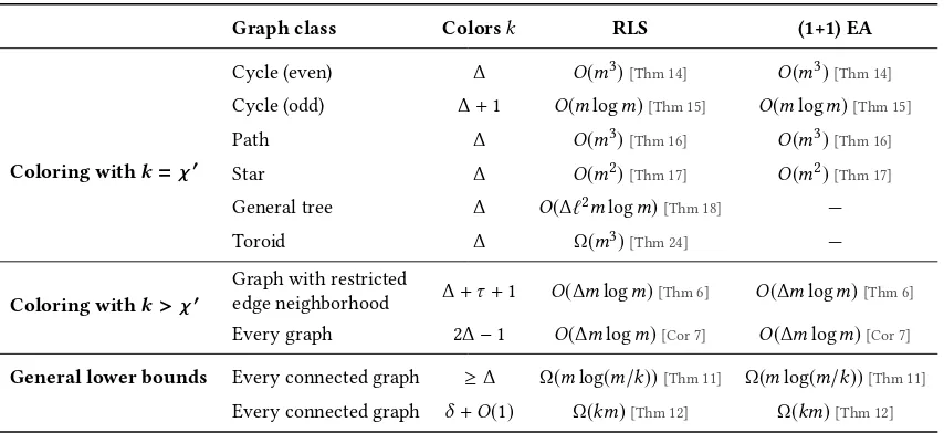
Table 1: Overview of presented results. Heremis the number of edges,∆the maximum degree,δthe minimum degree,ℓthe length of the longest simple path,kis the size of the color palette andχ′is the chromatic index. The lower bound for (bipartite) toroids holds for a worst-case initial coloring with two remaining conlicts. We conjecture an upper bound ofO(m3)for RLS on bipartite toroids from any initialization.
Graph class Colorsk RLS (1+1) EA
Coloring withk=χ′
Cycle (even) ∆ O(m3)[Thm 14] O(m3)[Thm 14]
Cycle (odd) ∆+1 O(mlogm)[Thm 15] O(mlogm)[Thm 15]
Path ∆ O(m3)[Thm 16] O(m3)[Thm 16]
Star ∆ O(m2)[Thm 17] O(m2)[Thm 17]
General tree ∆ O(∆ℓ2mlogm)[Thm 18] Ð
Toroid ∆ Ω(m3)[Thm 24] Ð
Coloring withk>χ′
Graph with restricted
edge neighborhood ∆+τ+1 O(∆mlogm)[Thm 6] O(∆mlogm)[Thm 6] Every graph 2∆−1 O(∆mlogm)[Cor 7] O(∆mlogm)[Cor 7]
General lower bounds Every connected graph ≥∆ Ω(mlog(m/k))[Thm 11] Ω(mlog(m/k))[Thm 11]
Every connected graph δ+O(1) Ω(km)[Thm 12] Ω(km)[Thm 12]
in case of bipartite graphs. For the Ising model/vertex coloring, Fischer and Wegener [11] showed that on cycle graphs RLS and (1+1) EA ind a proper 2-coloring in expected timeO(n3)andO(n2)
if crossover is used. Sudholt [25] considered the class of complete binary trees and showed that (1+1) EA needs exponential expected time, but a simple Genetic Algorithm with itness sharing and crossover locates a global optimum in expected cubic time. Sudholt and Zarges [26] studied the running time of an iterated local search (ILS) algorithm with diferent mutation operators based on color eliminations and Kempe chains (as in the algorithm of Misra and Gries). These operators recolor large connected parts of the graph. They showed that ILS with color eliminations eiciently computes 2-colorings in bipartite graphs while ILS with Kempe chains needs exponential time with overwhelming probability. Recently, Bossek et al. [5] studied vertex coloring in a dynamic setting where edges are added to a properly colored graph over time. Their results show that re-optimization can be much faster than optimization from scratch in certain situations. In contrast, adding edges in an unfavorable order may lead to even worse asymptotic running times than in the static setting.
In contrast to vertex coloring, the edge coloring problem has not been considered by the EA theory community, despite being a well-knownN P-hard problem with important applications. We address this problem here by providing rigorous runtime analyses of RLS and (1+1) EA for selected graph classes. We show that these algorithms are able to ind proper edge colorings eiciently for a range of graph classes. Our main results are gathered in Table 1.
This work is structured as follows. After formulating the founda-tions in Section 2 we given some general bounds in Section 3. We prove that a proper(2∆−1)-coloring can be found in expected time
O(∆mlogm)on arbitrary simple graphs with maximum degree∆, consider the expected time to ind colorings with few conlicts,
and formulate general lower bounds for general graphs. Next, we shift our focus to optimal colorings. In Section 4 we provide up-per bounds for simple graph classes, e. g., cycles, paths and star graphs. In Section 5 we show that on every tree the expected time to ind a proper coloring with∆colors is bounded from above by
O(∆ℓ2mlogm)in expectation whereℓis the length of the longest path in the tree. In Section 6 we discuss the analysis of toroid graphs as an example of a graph class with multiple cycles. Since the anal-ysis turns out to be surprisingly challenging, we only present a rigorous lower bound for a worst-case initialization and discuss the challenges involved in rigorously proving upper bounds. Section 7 joins theory and practice by conducting a series of experiments to (1) empirically back up our results, such as a conjecturedO(m3)
bound for toroids, and (2) to check assumptions on other, more gen-eral graph classes (e. g., hypercubes and complete graphs). Section 8 completes our irst excursion into edge coloring with concluding remarks and pointers to promising future research directions.
The appendix contains tools for the analysis of fair random walks used in the main part; our presentation of these largely known results may be of independent interest.
2
PRELIMINARIES
LetG = (V,E)be a simple undirected graph withn = |V|and
m=|E|. For an edgeewe denote by deg(e)the number of edges incident toeand byN(e)the set of edges incident toe. Note that for every graph with minimum degreeδand maximum degree∆
and every edgeewe have
2δ−2≤deg(e) ≤2∆−2.
We call a functionc:E→ {1, . . . ,k}anedge coloring/coloring
ofG. An edge coloringcis termedproperif no two incident edges share the same color, i. e.,∀e1,e2∈E:e1∩e2,∅ ⇒c(e1),c(e2). A graph isk-colorableif there is a proper edge coloring withkcolors. The smallest numberk, such thatGisk-colorable, is the so-called
chromatic indexand denotedχ′(G)or justχ′in the following. We call an edge pair(e1,e2)withe1,e2aconlictif the edges are incident and have the same color. Likewise, we call an edgeea
conlict edgeif there is at least one edge inN(e)that has the same color assigned. We shall often refer to the unique vertex shared betweene1ande2as thecommon vertexof the conlict. A coloriis termedfreeforeif no incident edge is colored withi.
2.1
Algorithms
In this work we consider the size of the color palette to be ixed to a parameterk ≥ χ′. The search space is thus given byS =
{1, . . . ,k}mand the itness function used is to minimize the number of conlicts, that is, the number of edge pairs that are conlicting. For example, if there are 4 edgese1,e2,e3,e4sharing a common vertex and all colored identically, they contribute 42
=6 conlicts to the itness.
Clearly, a solutionx∈Swith zero itness is a properk-coloring. We are interested in the expected number of function evaluations required until simple randomized search heuristics locate a proper coloring for the irst time. The algorithms under consideration are randomized local search (RLS, see Algorithm 1) and (1+1) EA (see Algorithm 2). Both algorithms maintain a single incumbent solution
x which is initialized uniformly at random. In each iteration the incumbent is subject to mutation and the mutantyreplacesxif it has no more conlicts. The only diference is in the mutation operator. While RLS recolors a single edge in each iteration with probability 1 (called alocal move), (1+1) EA recolors each edge with probability 1/mindependently. It thus has the ability to perform multiple local moves simultaneously.
Algorithm 1RLS
1: Generatex ∈ {1, . . . ,k}muniformly at random. 2: whileoptimum not founddo
3: Generateyby choosing an indexi∈ {1, . . . ,m}uniformly at random, choosing a new valueyi ∈ {1, . . . ,k}uniformly
at random and settingyj=xjfor allj,i. 4: Ifyhas no more conlicts thanx, letx :=y.
Algorithm 2(1+1) EA
1: Generatex ∈ {1, . . . ,k}muniformly at random. 2: whileoptimum not founddo
3: Generateyby deciding to mutate each edgexi with
prob-ability 1/m: if yes, choose a new valueyi ∈ {1, . . . ,k}
uniformly at random.
4: Ifyhas no more conlicts thanx, letx :=y.
Unless stated otherwise, RLS and (1+1) EA start with a coloring generated uniformly at random. Most of the upcoming positive results will hold for arbitrary initial colorings.
It should be noted that for reasons of clarity and consistency ś and because it seems to be more natural foredgecoloring ś all our runtime bounds are stated in terms of the number of edges,m, as opposed to the number of vertices.
2.2
On the Efect of Local Moves
To lay the foundations for the upcoming analyses, we explain the efect of local moves, before considering itness-improving and itness-neutral local moves (that is, local moves not altering the itness) in more detail.
Consider a local move at timetchanging the color of an edge
e ={u,v}fromitoj ,i. This move can only afect the status of edges inN(e) ∪ {e}.
Lete1,e2, . . . ,ekbe alli-colored edges inN(e)(if any). Then the
recolor operation will resolve all conlicts(e,e1),(e,e2), . . . ,(e,eℓ).
However, ife1′,e2′, . . . ,er′are allj-colored edges inN(e)(if any) then
the move will create conlicts(e,e1′),(e,e2′), . . . ,(e,er′).
It will be useful to regard conlicts as particles that can move through the graph. For example, if one previously conlicting edge pair(e,e′)becomes non-conlicting but another edge pair(e,e′′)
now becomes conlicting, we say that the conlict has moved from
(e,e′)to(e,e′′). If a local move atereduces the number of conlicts bys, we selectsconlicts involvinge uniformly at random and declare these to be resolved. The remaining conlicts (if any) are then declared to have moved.
This random selection is used to break symmetries and to ensure that every conlict has a fair chance to be removed in a itness-improving local move. For instance, ifN(e)contains twoi-colored edgese1,e2and onej-colored edgee1′then either the conlict(e,e1) moves to(e,e1′)and the conlict(e,e2)is declared resolved, or the conlict(e,e2)moves to(e,e′1)and the conlict(e,e1)is declared resolved. These decisions are made with equal probability.
2.3
On Possible Improvements
We irst collect some statements that allow us to identify possible improvements.
Recall that a coloriis called a free color for an edgeeif colori
does not appear in the neighborhood ofe. For every conlict(e1,e2), if either edgee1ore2has a free color, there is a local move that resolves the conlict.
The following lemma lower-bounds the number of free colors, or colors that only lead to one conlict.
Lemma 1. For every edgeethe following holds. Letkfreebe the number of free colors ateandkonethe number of colors that only
create one conlict among its incident edges, then
2kfree+kone≥2k−deg(e).
In particular, if there is no free color forethenehas at least2k−deg(e)
colors leading to one conlict only.
Proof. Note thatkonecolors account forkoneedges incident toe. Allkfreefree colors do not contribute any edges, but all remaining
k−kfree−konecolors contribute at least 2 edges. Since there are only deg(e)edges, we have
ByLemma 1 every edgeeinvolved in a conlict either has a free color or it has one other color that leads to one conlict. We refer to the latter color as analternative color.
For edges that are part of many conlicts, there is a larger proba-bility of reducing the number of conlicts.
Lemma 2. For every edgeethat is part of at least3conlicts there are at leastk−∆+⌈(∆−1)/3⌉other colors forethat lead to at most 2 conlicts.
Proof. There are at most2∆−2edges incident toe. There can be at most⌊(2∆−2)/3⌋colors that also lead to 3 (or more) conlicts.
Thus there must bek−1− ⌊(2∆−2)/3⌋ ≥k−∆+(∆−1)/3other colors that have at most 2 conlicts. Since the number of colors is an integer, it is at leastk−∆+⌈(∆−1)/3⌉as claimed. □
Conlicts can be resolved in case two or more conlicts of the same color are incident.
Lemma 3. For every graphGwith maximum degree∆, for every
conlict(e1,e2)the following holds. If the conlict is incident to another
conlict(e3,e4)of the same color, with probability at least1/(2km)
the conlict(e1,e2)is resolved in the next step.
Proof. Note that edgese1,e2,e3,e4may not be mutually
difer-ent, however we know thate1,e2,e3,e4ands:=Ð4i
=1{ei}
≥3
as we are dealing with two diferent conlicts. We consider the fol-lowing cases:
(1) The union of the two conlicts contains a path of length at least 3.
(2) The two conlicts share a common center vertex.
Note that these are the only cases since the absence of a path of length at least 3 implies that all edges must have one vertex in common.
In the irst case, the middle edge of that path can be recolored with another color that only creates at most 1 conlict. By Lemma 1 this reduces the number of conlicts. Since we may create a new conlict, the conlict(e1,e2)may either be declared as resolved, or
declared to have moved to the new conlicting edges. Since there are at least 2 conlicts afected by the recolor operation, one of these will be chosen uniformly at random to be declared to have moved. So with probability at least1/2, conlict(e1,e2)will be declared as
resolved.
In the second case, each of thesedges inÐ4
i=1{ei}is involved
in at leasts−1≥2conlicts. According to Lemma 1, recoloring an edge in{e1,e2}with a free or an alternative color will make at
least 2 edge pairs non-conlicting (including(e1,e2)) while making
at most one non-conlicting edge pair conlicting. As above, the probability that(e1,e2)will be declared resolved is at least1/2. □
2.4
Fitness-Neutral Operations
We also describe and characterize some itness-neutral operations.
Deinition 4. Let(e1,e2)be a conlict at timetand let(e1′,e2′),
(e1,e2)be the same conlict at timet+1. We say that the conlictwas
rotatedat timetif the common vertex has not changed:e1∩e2=
e1′∩e2′. Otherwise, that is, if the common vertex has changed to a neighbouring vertex, we say that the conlicthas moved.
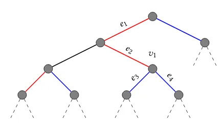
v1
e1
e2
[image:5.612.326.544.72.192.2]e3 e4
Figure 1: Example of a blocked conlict (e1,e2). Here, it is
blocked by another conlict(e3,e4)and cannot move further
down.
The following lemma establishes that conlicts can move in the graph unless they are blocked by other conlicts.
Lemma 5. Consider a conlict(e1,e2). Letv1be the end point ofe1
not shared withe2. If there is no conlict that hasv1as shared vertex
thene1has a free color or an alternative color that, when applied,
leads to the conlict being moved, withv1as the new shared vertex.
The same statement also holds with the roles ofe1ande2swapped.
Proof. W. l. o. g.e1has color 1. Callvthe unique joint vertex in
e1∩e2. We pessimistically assume thate1has no free color as
other-wise the statement is trivial. By Lemma 1 (and excluding the color
c(e1)itself)e1hass:=2k−deg(e) −1 alternative colors, w. l. o. g. color 2. We prove the statement by contraposition. Assume that all these alternative colors lead to the conlict being rotated. Then for all alternative colorsi∈A(e1), there is exactly onei-colored edge atvand there is noi-colored edge atv1, as otherwiseiwould not be an alternative color fore1.
This means that the number of colors used atv1 is at most
k−(2k−deg(e)−1)=deg(e)−k+1=(deg(v1)+deg(v)−2)−k+1≤ deg(v1) −1. By the pigeon-hole principle, there must be at least one color that appears at least twice atv1. This completes the contraposition. Hence if there is no conlict withv1as shared vertex, there must be an alternative color fore1that moves the conlict along the edgee1, withv1as new shared vertex. □
The requirements of Lemma 5 are necessary. Assume there is an-other conlict(e3,e4),e3,e1ande4,e1, withe1's only alternative colorc(e3),c(e1)(assuminge1only has one alternative color) and
v1as its common vertex (see Figure 1). Then recoloringe1with its alternative colorc(e3)yields two conlicting edge pairs,(e1,e3)and
(e1,e4). Unless there are furtherc(e1)-colored conlicts involving
e1, this move leads to a decrease in itness and will be rejected by RLS. We say that then the conlict(e1,e2)isblockedby the conlict
(e3,e4).
3
GENERAL BOUNDS
3.1
(
2∆
−
1
)
-Coloring Arbitrary Graphs
Theorem 6. On every graphG=(V,E)with maximum degree∆
andmaxe∈Edeg(e) =∆+τ for0 ≤τ ≤∆−2, for every initial coloring, RLS and (1+1) EA ind a proper coloring withk=∆+τ+1
colors in expected timeO(∆mlogm).
Proof. First note that given a color palette of sizek=∆+τ+1 for each conlict edge there is always at least one free color. Now letXt ∈Ndenote the number of conlicts andXt(e)the number
of conlicts edgeeis part of at timet. Clearly,Xt ≤ m2 =xmax and ś since every edge is counted twice śÍ
eXt(e)=2Xt. With
probability at least 1/(ekm), (1+1) EA resolves allXt(e)conlicts
the edgeeis involved in. This lower bound does hold for RLS, too. As a consequence we get
E(Xt+1|Xt) ≤Xt−
Í
eXt(e)
ekm =Xt−
2Xt
ekm =Xt
1−ekm2
.
This implies an expected drift of
E(Xt−Xt+1 |Xt) ≥Xt
2
ekm
.
At last we apply the multiplicative drift theorem [9] and obtain a runtime bound of
ekm
2 ln(1+O(m 2))
=O(∆mlogm).
The inal equality is due tok=Θ(∆). □
Note that every simple graph admits a proper coloring with 2∆−1 colors, since deg(e) ≤2∆−2 for all edges. Hence, setting
τ=∆−2 in Theorem 6 we obtain the following result.
Corollary 7. On every graph with maximum degree∆and for
every initial coloring, RLS and (1+1) EA ind a coloring withk=2∆−1
colors in expected timeO(∆mlogm).
3.2
Reducing the Number of Conlicts
The number of conlicts (that is, the number of conlicting edge pairs) can be as large as m2
=Θ(m2)for a star graph or a complete graph where all edges have the same color. We show that, for every number of colorsk≥∆and every initial coloring, the number of
conlicts quickly decreases to at mostm.
Theorem 8. For every graphGwithmedges and maximum de-gree∆and every initial coloring, the expected time until RLS or
(1+1) EA withk ≥ ∆colors have found a solution with at mostm
conlicts isO(mlogm).
Proof. LetXt again denote the number of conlicts at timet
andXt(e)denote the number of conlicts edgeeis part of at timet. For edgesewithXt(e)>2, Lemma 2 states that there are at least
k−∆+⌈(∆−1)/3⌉alternative colors which lead to at most two
conlicts. The probability of executing a local move ateis at least 1/(em)for both RLS and (1+1) EA and the probability to recolor the sampled edge with one of these colors is at least
k−∆+⌈(∆−1)/3⌉
k =1−
∆− ⌈(∆−1)/3⌉
k
≥1−
∆
− ⌈(∆−1)/3⌉
∆
≥ 14.
Here, the last inequality stems from the observation that the term in braces is maximal for∆ = 4. Thus, ifXt(e) > 2 then with
probability at least 1/(4em)we getXt(e) −Xt+1(e) ≥Xt(e) −2. The
same statement holds trivially forXt(e) ≤2 as a local move ate
cannot increase the number of conlicts. As long asXt ≥m+1, the overall expected drift is thus
E(Xt−Xt+1|Xt) ≥
Õ
e
1
4em· (Xt(e) −2)
=41
em Õ
e
Xt(e) −2m
!
=4em1 (2Xt−2m).
The variable drift theorem [16] (Theorem 3 in [17]) then yields an upper bound of
2em+
∫ m2
m+1 4em
2x−2m dx
=2em+4em
∫ m2
m+1 1 2x−2mdx
=2em+4em
ln
(2x−2m)
2
m2
m+1
=2em+4em
ln
(2m2−2m)
2 −
ln 2 2
≤2em+4emlnm. □
We remark without proof that within expected timeO(∆mlogm), both RLS and (1+1) EA ind a solution with at mostm/2 conlicts, for every graph withmedges. This can be shown by waiting for free or alternative colors to be applied, similarly to the proof of Theorem 6.
3.3
General Lower Bounds
To complement our upper bounds and to establish a baseline for good performance, we now turn to proving lower bounds for RLS and (1+1) EA. We show two lower bounds that apply to arbitrary connected graphs. As a irst step, we show that the initial coloring hasΘ(m/k)conlicts with high probability.
Lemma 9. For every connected graph withmedges, if an edge coloring is chosen uniformly at random with colors{1, . . . ,k}then there are at leastm/(4k)conlicts on mutually disjoint edges, with probability1−e−Ω(m).
To show Lemma 9, we irst show the following combinatorial result.
Lemma 10. Every connected graph withmedges admits a sequence of mutually disjoint edgese1, . . .e2⌊m/2⌋ such that for alli with 1≤i≤ ⌊m/2⌋,e2i−1ande2iare incident edges.
Proof. We prove the claim by induction overm. The claim is trivial form≤1. Assume that the claim holds form−2 and consider any connected graphGwithm≥2 edges.
Consider a spanning treeTofGrooted at an arbitrary but ixed vertex and denote by degT(v)the degree of a vertexv inT. We consider leaves inT that have a maximum graph distance from the root in the subgraph induced byT and call thesedeepest leaves.
connected viaTand hence we can decompose the remaining graph ofm−2edges inductively into⌊(m−2)/2⌋=⌊m/2⌋ −1further edge pairs.
Otherwise, if there is a deepest leafu, with a parent that we callv, that is incident to exactly one edgeenot belonging toT, we removeeand{u,v}and the graph remains connected viaT\ {u,v}
sinceuis a leaf inT. The remaining graph can then be decomposed inductively.
Otherwise all deepest leaves inT are also leaves inG. Fix a deepest leafuwith a parent that we callv. Ifuhas a siblingu′in the tree thenu′must be another deepest leaf asuwas chosen to have a maximum graph distance to the root. Then the edges{u,v}
and{u′,v}are incident. Removing these edges leaves a connected graph withm−2edges, which can be decomposed inductively.
Ifudoes not have a sibling inT then, since there are at least2
edges in the graph,vmust have a parent in the tree that we callw. We note that{u,v}and{v,w}are incident, and removing them from the graph leaves a connected graph as there are no further edges atunorv. Removing{u,v}and{v,w}and decomposing the remaining graph inductively as above completes the proof. □
Proof of Lemma 9. By Lemma 10 there is a sequence of mu-tually disjoint edgese1, . . . ,e2⌊m/2⌋such that edgese2i−1ande2i
are incident, for all1 ≤i ≤ ⌊m/2⌋. For each such edge pair the probability that the two edges will be conlicting after a random initialization is1/k. These events are independent for all edge pairs, hence we can apply Chernof bounds. This yields that, with proba-bility1−e−Ω(m), at leastm/(4k)edge pairse2i−1,e2iare conlicting
after initialization. □
The following lower bound follows now from Lemma 9 and standard coupon collector arguments.
Theorem 11. The expected time for RLS or (1+1) EA to ind a properk-coloring on any connected graphG, for any value ofk≤m, isΩ(mlog(m/k)). This isΩ(mlogm)ifk=O(m1−Ω(1)); this is the
case, for example, for all regular graphs or graphs whereδ=Ω(∆).
Proof. By Lemma 9, with probability 1−e−Ω(m), the initial coloring has at leastm/(4k)conlicts on mutually disjoint edges. Assume that this happens and ix a conlicting pair. The conlict can only be resolved if one of the two edges is being picked during mutation. The probability for this event is at most 2/mfor both RLS and (1+1) EA.
The probability that a ixed conlicting pair is not resolved within
t:=(m/2−1)ln(m/(4k))mutations is at least
1−m2
t
≥e−ln(m/(4k))=4mk.
The probability that there is a conlict out of them/(4k)conlicts that is not resolved after timetis at least
1−
1−4mk
m/(4k)
≥1−1e.
This means that the expected optimization time is at least(1−1/e−
e−Ω(m)) ·t=Ω(mlog(m/k)). □
Theorem 11 shows that the upper bound from Corollary 7 is asymptotically tight if∆=O(1)as then log(m/k)=Θ(logm).
We also give a lower bound that includes a factor ofk(but no logmfactor).
Theorem 12. The expected time of RLS and (1+1) EA to ind a properk-coloring on any connected graph with minimum degree δ ≥2andδ ≤k≤mis at leastΩ(km/(k−δ+1)). This isΩ(km)
ifk=δ+O(1), for example when the graph is∆-regular andk ∈
{∆,∆+1}.
Proof. By Lemma 9, the probability of initializing with an opti-mal solution ise−Ω(m).
The best case situation for inding a proper coloring is attained when there is just one conlict(e1,e2), or two conlicts that share an edgee1and form a path of 3 edges. This is because if there are two conlicts with disjoint edge pairs, or multiple conlicts that have the same vertex as common vertex, multiple speciic edges need to be recolored to ind the optimum in one step. This is impossible for RLS and has probabilityO(1/m2)for (1+1) EA.
To ind a proper coloring from a coloring with just one conlict, it is necessary to recolore1ore2. For any such edgee, since there are no other conlicts, at leastδ−1 colors are taken, hence the number of free colors is at mostk−δ+1. The probability to recolor one of the two involved edges and to pick a free color is at most 2(k−δ+1)/(km)and the expected waiting time for this event is at leastkm/(2(k−δ+1)).
In the case of two conlicts with a shared edgee1,e1must be recolored with one ofk−δ+1 free colors, which has probability at most(k−δ+1)/(km). The expected waiting time in this case is
at leastkm/(k−δ+1). □
Together, we obtain the following result for∆-regular graphs.
Corollary 13. The expected time for RLS and (1+1) EA to ind a proper coloring on any∆-regular connected graph, withk≤∆+O(1), isΩ(∆m+mlogm).
4
RUNTIME BOUNDS FOR SIMPLE GRAPH
CLASSES
We now consider the performance of RLS and (1+1) EA on a range of simple graph classes. We start with cycle graphs, that is, graphs that consist of a single cycle visiting all vertices.
Theorem 14. For every initial coloring, the expected time for RLS and (1+1) EA to ind a proper 2-coloring on every cycle graphC2n
with an even number of nodes isO(m3).
Proof. We irst review the notion of aline-graphL(G)of an arbitrary graphG. The line-graph is a graph with one node for each edge ofGand an edge between nodes if and only if the corre-sponding edges inGare incident. It is easy to see that an optimal edge-coloring ofGcorresponds to an optimal vertex-coloring of
ofO(m3)for edge-coloring ofC2n with 2 colors. The key idea of
[11] is to consider connected monochromatic blocks and the length of the shortest block in particular. They estimate the number of so-called relevant steps, i. e., steps that either decrease the number of monochromatic blocks or the length of the shortest block by
O(n2). The key argument is that the algorithms need to overcome plateaus of length at mostn/2. Here, random walk arguments yield the quadratic bound. Sincensuch steps are suicient we end up with a runtime bound ofO(n3)=O(m3). □
Note that cycle graphs with an odd number of edges do not admit a proper 2-coloring and hence at least three colors are needed. The additional color makes the problem much easier, because there is always a free color for a conlicting edge.
Theorem 15. For every initial coloring, the expected time of RLS and (1+1) EA to ind a proper 3-coloring on a cycle graphC2n+1with
an odd number of nodes isO(mlogm).
Proof. Note that inC2n+1we have 2∆−1=3 and hence the theorem follows directly from Corollary 7. □
We also note for completeness that paths can be colored in the same way as even cycles, with almost identical proofs.
Theorem 16. For every initial coloring, the expected time of RLS and (1+1) EA to ind a proper 2-coloring on a path withmedges is O(m3).
Proof. Follows the same arguments as the proof of Theorem 14. □
Now we consider star graphs, deined as a graph with a vertex in the center of the graph, to which all edges are incident. This implies∆=m.
Theorem 17. The expected time of RLS and (1+1) EA to ind a proper coloring withk=∆=mcolors on a star graph withmedges
is bounded byO(m2).
Proof. Consider the number of conlictsXt at timet ∈ N0 and denote byXt(i)the number of edges colored with colori ∈ {1, . . . ,m}at timet. Note thatXt(i) ≥ 1 implies that there are (Xt(i) −1)edges which shall be colored diferently with free colors.
Note further that
Xt =
m
Õ
i=1
Xt(i)
2
=12
m
Õ
i=1
Xt(i) · (Xt(i) −1).
Call the total number of free colorss. With the considerations from above we can concludes=Ími=1max{0,Xt(i) −1}. The
max-function ensures that colors that are not used so far do not have a negative contribution tos.
Note that in bothXt andsall valuesXt(i) ≤1 lead to a
con-tribution of 0, hence we can focus on valuesXt(i) ≥ 2. Using
Xt(i) ≤2(Xt(i) −1)forXt(i) ≥2,
Xt=12
Õ
i:Xt(i)≥2
Xt(i) · (Xt(i) −1)
≤ Õ
i:Xt(i)≥2
(Xt(i) −1)2
≤ Õ
i:Xt(i)≥2
(Xt(i) −1)
2
=
Õ
i:Xt(i)≥2
max{0,Xt(i) −1}
2
=s2,
where the last inequality follows from the Cauchy-Schwarz inequal-ity. We conclude thats≥√Xt.
IfXt >1 we can improve by selecting a single edge and
recol-oring this edge with a free color. This happens with probability at leasts/(ekm) ≥s/(em2)for both RLS and (1+1) EA. Hence, the overall expected drift is
E(Xt−Xt+1|Xt) ≥ 1
2
m
Õ
i=1
Xt(i) · (Xt(i) −1) ·
s
em2
=Xt·
s
em2
≥X
3/2
t
em2.
Withxmin=1≤Xt ≤ m2<m2the variable drift theorem yields
an upper bound of
em2+
∫ m2
1
em2
x−3/2dx
=em2+em2
∫ m2
1
x−3/2dx
=em2+em2
−√2
x m2
1
= em2+em2
2− 2
m
≤3em2−2em=O(m2). □
5
A BOUND FOR TREES
We now show that RLS can eiciently edge-color arbitrary trees with∆colors. We focus on RLS instead of (1+1) EA as the analysis
becomes more involved. Even on simple graphs such as cycles, Fischer and Wegener's work shows that the analysis of (1+1) EA becomes way more complicated than that of RLS [11] and it is not clear whether (1+1) EA has any advantage over RLS (we shall revisit this question experimentally, in Section 7).
Theorem 18. On every treeGwithℓ:=ℓ(G), RLS withk =∆
inds a proper∆-coloring in expected timeO(∆ℓ2mlogm).
Proof. Lethbe the height of the tree, i. e., the length of the longest simple path from the root to any leaf. Note thath≤ℓ≤2h, hence we only need to show an upper bound ofO(∆h2mlogn). For
a vertexvdenote byd(v)the depth ofv, that is, the length of the unique simple path fromvto the root.
color of the conlict taggedi. Deineφt(i):=h−d(vt(i)), where
vt(i)denotes the common vertex of the conlict taggediat timet. If
the tag has disappeared from the graph, we deineφt(i):=0. Note that, while the tag is active,1≤φt(i) ≤has the common vertex of
any conlict cannot be a leaf, hence0≤d(vt(i)) ≤h−1.
By Lemma 5, a conlict can move up or down in the tree as long as it is not blocked by another conlict (see Figure 1 for an example of a blocked conlict). While there is no blocking conlict, there is only at most one recolor operation that would move a conlict closer to the root, thus increasingφt, while there is at least one
recolor operation that would move it away from the root, thus decreasingφt. Whileφt(i)=1the conlict has reached a leaf and can be resolved by recoloring the edge incident to the leaf. However, blocking conlicts complicate the situation as they can eliminate moves that decreaseφt. On the other hand, the blocking conlict
has an advantage as it does not have any moves that can increase
φt. We address this by considering the following model that relects
how conlicts move through the tree.
Consider a conlict taggediand an edgeethat connects levels
d(vt(i))andd(vt(i)+1). Assume thateis incident to both edges of another conlict taggedjon levelsd(vt(i)+1)andd(vt(i)+2). If a recolor operation picks edgeeand colorc(j)then weswap tagsi andj. This is done regardless of whether the recolor operation is ac-cepted or not. The idea behind this swap is that while a conlict may be blocked by another conlict, tags can roam more freely. We will show in the following that theφt-values of tags are stochastically
dominated by a fair random walk.
Lemma 19. For every tagiwe have
Pr(φt+1(i)=φt(i)+1) ≤ km1 .
Proof. A tag can only move up under the following conditions. If the two edges of conlictiare on the same level, the only way the tag can move up is if it is swapped with a tag higher up in the tree. This requires a speciic recolor operation that occurs with probability 1/(km).
If the two edges of the conlict are on diferent levels, tagicannot be swapped łupwardsž, but a recolor operation can move the conlict up. Lete1be the upper edge of the conlict ande2be the unique edge incident toe1on the level above. For a recolor operation to move the conlict up,e1must be recolored with colorc(e2). This operation has probability 1/(km). □
Lemma 20. For every active tagiwe have
Pr(φt+1(i) ≤φt(i) −1) ≥
1
km.
Proof. Consider an edgee ={v1,vt(i)}of the conlict where
d(v1)=d(vt(i))+1.
First assume thatehas a free color. Note that this is implied by
φt(i)=1 as theneis incident to a leaf; since two edges atvare coloredc(i)and deg(e)=deg(v) ≤∆there must be a free color by the pigeon-hole principle. Choosing a free color would remove the tag, yieldingφt+1(i)=0≤φt(i) −1. The probability of applying a
free color toeis at least 1/(km).
Now assume thatehas no free color, which impliesφt(i) ≥2. By
Lemma 5, if there is no other conlict that hasv1as shared vertex, there must be a free color or an alternative color that moves the
conlict further down in the tree, leading toφt+1(i)=φt(i) −1. The
probability for this event is at least 1/(km).
Finally, we assume thatehas no free color but there is a conlict taggedjwithv1as shared vertex. We consider two sub-cases. First assume thate is incident to at least 2 edges of colorc(i). Then, arguing similarly to Lemma 3, there must be two colors that, when applied toe, only lead to one conlict that involvese. More formally, letxbe the number of colors that appear at least twice. Then if there is no free color the number of edges incident toemust respect
x·2+(k−x) ·1 ≤ 2∆−2, which is equivalent tox ≤ ∆−2. With probability at least 1/2, conlictiwill be declared resolved (cf. Section 2.2). The probability for these events is at least 2/(km)·1/2= 1/(km).
Ifeis only incident to one edge of colorc(i)(the other edge of conlicti) then trying to recolorewith colorc(j)will be rejected as it would increase the number of conlicts. However, it would swap tagsiandjand, consequently,φt+1(i)=φt(i) −1. The probability for this recolor operation is 1/(km). □
We conclude thatφtis dominated by a lazy2fair random walk on {0, . . . ,h}where the probability of changing the current state is at least 1/(km). By the irst statement of Lemma 27 in the appendix, the expected time to reach state 0 is at mosth2km. Since there are up to
m2fair random walks for all tags (which are not necessarily indepen-dent), the third statement of Lemma 27 yields that the expected time for all tags to disappear isO(h2kmlog(m2))=O(h2kmlogm). □
6
TOWARDS AN ANALYSIS OF TOROIDS
We now turn our attention to the performance of RLS on toroids, which are essentially two-dimensional grids with edges łwrapping aroundž. The reason for studying toroids is that they represent a simple graph class featuring many cycles. We will see in the following that cycles play a key role in edge coloring, and that the analysis can become quite involved. We believe that many of the arguments applied to bipartite toroids also apply to general∆-regular bipartite graphs, or even arbitrary bipartite graphs.
Toroids are formally deined as graphs with vertices(i,j)for 1≤i≤n1and 1≤j ≤n2and edges from(i,j)to vertices(i+1,j),
(i−1,j),(i,j+1)and(i,j−1), where for ease of notation we identify indices 0 withn1andn1+1 with 1 for the irst argument and likewise forn2and the second argument. The number of vertices in a toroid isn1·n2.
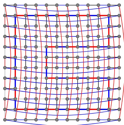
We imagine a toroid drawn as a 2-dimensional grid, with edges wrapping around, such that edges are drawn either horizontally or vertically (see Figure 2 for an example). We speak of rows and columns in an obvious way.
Note that a toroid with parametersn1,n2is bipartite if bothn1 andn2are even. We always assume thatn1,n2 ≥4 as then the toroid is 4-regular, that is, every vertex has degree 4. This implies that the number of edges ism=2n. In the following, we tacitly assume that all toroids are 4-regular.
Bipartite toroids are 4-edge-colorable, and the number of proper colorings is exponential. For example, all colorings where rows are colored with alternating colors 1 and 2 (say) and columns are colored with alternating colors 3 and 4, are proper colorings. For
each row and column we can choose independently which of the two colors comes irst, which gives rise to2n1+n2diferent proper
colorings. There are many further proper colorings that do not follow patterns of rows and columns (see Figure 2 for a coloring that is nearly proper). Note that, sincek=4colors are used and toroids arek-regular, every vertex in every proper coloring must be incident to exactly one edge of each color. The orientation of these edges can vary between neighboring vertices.
For improper colorings we show that there exist unique paths of alternating colors that start and end in a common vertex of a conlict. We refer to a simple path asi-j-pathif colorsiandjare alternating on the path.
Lemma 21. Consider a conlict(e1,e2)with coloriand common
vertexv, wheree1={v1,v}ande2 ={v,v2}. Then the following
statements hold:
(1) For all colorsj,i, there is a uniquei-j-path that starts atv, usese1but note2and ends in a vertexwthat is the common
vertex of a conlict. The same holds when the roles ofv1and
v2are swapped.
(2) For all colorsj ,i, the uniquei-j-path starting withe1does
not share any edges with the uniquei-j-path starting withe2.
(3) Alli-j-paths wherej is a free color atv end in a diferent conlict.
Proof. We follow thisi-j-path, starting fromvand moving tov1.
For every vertexuon this path, the following holds. Ifuhas more than one incident edge coloredjoruhas more than one incident edge coloredi,w=uand the claim holds. Ifuonly has one incident edge colorediorj, by the pigeon-hole principleumust have two incident edges of a diferent color and we can takew =u. If the above cases do not occur,uhas exactly onei-colored edge and onej-colored edge, and the path can be extended, while remaining unique.
The path cannot have any loops, hence it must reach a conlict without using edgee2or return tovviae2. We show that the latter
case is impossible. Assume for a contradiction that it returns tov
viae2, closing a cycle. Then the irst and the last edge of the path
were coloredi. Since colors must alternate on the path, the cycle must have odd length, contradicting the assumption that the toroid is bipartite. Hence the path must end in a conlict without usinge2.
This argument also shows that the uniquei-j-path starting with
e1has no common edges with the uniquei-j-path starting withe2,
proving the second statement.
For the third statement, ifjis a free color atv, there can be no
i-jpaths looping back tovas the last edge cannot be coloredj(asj
is a free color atv) nori(as it would close an odd cycle). □
Lemma 21 in particular implies that every improper coloring must have at least two conlicts.
The following lemma shows that conlicts can move alongi-j
paths, whereiis the color of the conlict andj is a free color at its common vertex. After one such step, the roles ofiandj are swapped. A requirement for the lemma to hold is that no other conlicts interfere.
Lemma 22. Consider a conlict(e1,e2)with coloriand common
vertexv, wheree1 ={v1,v}ande2 ={v,v2}. Assume there is no
other conlict that hasv,v1orv2as common vertex. Then
(1) there is a unique free colorjatv
(2) the only accepted moves involving the conlict(e1,e2)are those
wheree1ore2respectively is recoloredj
(3) after such a move is applied, the conlict has colorjandiis a free color at its joint vertex.
Proof. There must be a unique free color atvsince deg(v)=4 and the two remaining edges must have diferent colors to each other and diferent fromi(as otherwise there would be another conlict withvas common vertex). Let the free color bej.
Since there is no conlict withv1as common vertex, all colors must be present exactly once atv1. The same holds forv2.
Ife1is recoloredjthene1ande2stop being conlicting, ande1 starts being conlicting with the uniquej-colored edge atv. This is a itness-neutral move that moves the conlict towards a new joint vertexv1.
Ife1is recoloreds∈ {1, . . . ,c}\{i,j}then the number of conlicts increases as there is ones-colored edge atv1and anothers-colored edge atv. Hence the only accepted move fore1is to recolor is withj, the free color atv.
All the above holds analogously fore2, completing the proof of the second statement.
The third statement holds since, before applying the move,e1and
e2are the onlyi-colored edges atv1andv2, respectively. When one of these edges is recolored,ibecomes a free color at the respective
vertex. □
We also characterize edges that cannot be recolored as they lead to rejected moves.
Lemma 23. Consider an edgeethat is not part of any conlict. If e has an end point where all other colors are present then all local moves recoloringewill be rejected.
Proof. Lete={u,v}and w. l. o. g. let all other colors be present atv. Sinceeis not part of any conlict, no conlicts will be resolved by recoloringe. However, a new conlict will be created withvas common vertex. Thus the number of conlicts will increase and the
move will be rejected. □
In the following, we consider the time to resolve the last two remaining conlicts. We show a lower bound ofΩ(m3)when starting
with a particular coloring with just two conlicts. Then we argue why we believe that this bound is asymptotically tight and why this is diicult to prove formally.
Theorem 24. For every bipartite toroid, there is a search point with just two conlicts from which RLS withk=4colors needs expected
timeΩ(m3)to ind a proper 4-coloring.
Proof. A cycle is calledchordlessif no two vertices are con-nected by an edge that does not itself belong to the cycle (the cycle highlighted in Figure 2 is chordless).
Figure 2: Sketch of a worst-case initial coloring for toroids. The cycle drawn in bold uses only colors red and blue, with colors alternating, bar two conlicts.
gaps that the remainder of the graph can still be properly colored.) Figure 2 shows an example. Note that the construction can easily be scaled up for larger graphs by duplicating rows and/or columns appropriately.
Call the common vertices of the two conlictsv1andv2,
respec-tively. We have twoi-j-paths betweenv1andv2that together form
the cycleC, whereiandjare the colors of the conlicts and the free colors atv1andv2. We call these pathsaugmenting paths(inspired
by well-known algorithms for maximum matchings and subsequent studies of EAs [13]) as swapping colors on all edges of the path yields a itness improvement (and in this case, a proper coloring). We shall pay particular attention to the length of the shortest augmenting path. Once this length has reduced to 1, RLS is able to recolor this edge and, if the right color is chosen, this yields a proper coloring. The idea of considering the shortest augmenting path is borrowed from Fischer and Wegener's analysis of coloring problems on cycle graphs [11]. On the cycleC, the length of the shortest augmenting path corresponds to the graph distance ofv1
andv2on the subgraph induced byC.
By Lemma 23, as long asv1andv2are not adjacent on the cycle,
only local moves at the conlicting edges will be accepted. This is because the cycle is chordless andv1andv2can only be adjacent if
they are adjacent on the cycle. All other vertices have edges of all four colors, thus every non-conlicting edge meets the conditions of Lemma 23. In other words, the only accepted moves are those moving one of the conlicts along the cycle, unless the conlicts' common vertices have reached a distance of 1. Once this happens, we pessimistically assume that a proper coloring has been found.
Both conlicts can travel in either direction with equal probability
1/(km). This implies that, if the length of the shortest augmenting path is less than|C|/2, there are two local moves that reduce this length by 1, and there are two local moves that increase this length
by 1. If the maximum possible length of|C|/2is reached3, there are 4 local moves that decrease the length of the shortest augmenting path.
Hence the process can be regarded as a fair random walk on states{1,2,3, . . . ,|C|/2}with a relecting state|C|/2and transition probabilities to neighboring states of2/(km)(and4/(km)in the case of|C|/2). With the remaining probability, the random walk stays put.
Since|C| =Θ(m), the initial distance isΘ(m), and transitions happen with probability4/(km), by Lemma 27 the expected time
to reach state 1 isΘ(m3). □
It seems plausible that the last non-optimal itness level is the most diicult one, in the worst case. We conjecture that the lower bound from Theorem 24 is tight and that the last non-optimal itness level is optimized in expected timeO(m3)for all colorings with two conlicts remaining. We do not have a formal proof for this conjecture for reasons explained in the following.
Call the common vertices of the two conlictsv1 andv2. By
Lemma 21 there are two uniquei-j-paths connectingv1 andv2
that form a cycleC. As in the proof of Theorem 24 we consider the length of the shortest augmenting path, or equivalently the graph distance between the conlicts' common vertices onC. The proof of Theorem 24 has already established an upper bound ofO(m3)
for reaching a state 1, assuming thatCis chordless. Note that from state 1 there is a probability of at least1/(km)=Ω(1/m)of inding the optimum in the next step. There is also a probability of at most
3/m=O(1/m)of making any other accepted move (for instance, increasing the current state) as in this situation, by Lemma 23, only moves afecting one of the 3 edges that are part of a conlict may be accepted. Hence, there is a constant probability that the optimum will be found within the nextO(m)steps before any other accepted move is made. If this is not the case, we repeat the above arguments. Thus, if suices to bound the expected time to reach state1by
O(m3).
A problem arises ifCis not chordless and ifv1andv2are
con-nected by an edge not onC. Leta < {i,j}denote the color of
{v1,v2}. Both conlicts must have the same colorias otherwise
every path betweenv1andv2would have even length and the edge
{v1,v2}would close an odd cycle. But in this situation the edge
{v1,v2}can be recoloredjin a itness-neutral operation asjis a
free color for bothv1andv2(note that Lemma 23 does not apply).
This means that the free color at bothv1andv2switches fromj
toa, and there is a corresponding cycleC′with alternating colors
i-abetweenv1andv2on which the conlicts are able to move. Note
that the colors may switch back toiandjat{v1,v2}4, but the colors
might also switch again towards arbitrary combinations of colors on further cyclesC′′,C′′′, and so on.
The same efect may happen even in chordless cycles when the distance of the shortest augmenting path has reduced to 1. Then the edge{v1,v2}is incident to two edges of the two colors diferent
fromiandj. Recoloring the edge with such a color is a itness-neutral move as it removes the two conlicts onC, while creating two new conlicts with joint verticesvandw. This switches the
3Note that|C|/2is an integer asCmust be of even length.
4In other words, if we consider the state graph of all possible colorings that can be
random walk to another cycleC′, while the length of the shortest augmenting path remains at 1. Even ifCwas chordless,C′may not be chordless. Hence, to get a rigorous upper bound ofO(m3)for the last itness level, we would have to assume that all cycles that can ever be reached are chordless.
The situation is complicated further when more than two con-licts are present. Other concon-licts may interfere with the process described above in various ways:
•They can block augmenting paths at one end. While this is the case (and no other interference happens), one end of the augmenting path will be ixed, while the other end can perform a random walk. Then the previous random walk arguments can still be applied with transition probabilities reducing from2/(cm)to1/(cm).
•Augmenting paths may become blocked at both ends, in which case they cease to be łaugmentingž. For trees we used the idea of tags being swapped, so that tags could roam more freely even though the original conlicts were being blocked. Tags could always be removed when reaching leaves. It is not clear whether or how this idea can be applied for toroids as we are lacking conditions on when tags will disappear.
•If two conlicts share the same common vertexv, there are two free colors atv, possibly increasing the number of aug-menting paths.
•Augmenting paths that are blocked can become unblocked, which may suddenly and drastically increase the length of the shortest augmenting path.
It seems plausible that search points with many conlicts have many augmenting paths. However, proving this does not seem ob-vious, even when we consider paths that are blocked on exactly one end as augmenting paths. Even proving that a single augmenting path exists is not obvious. It is possible to construct colorings where several conlicts all block each other on both ends. Hence, it is an open problem to prove or disprove that in every improper coloring there exist conlicts that are not blocked on both ends.
Note, however, that even if all conlicts end up being blocked, it may still be likely that conlicts become unblocked once other con-licts have moved about. And all the above considerations arise from a worst-case perspective, and trying to prove statements that apply toeveryimproper coloring. Observing simulations suggests that blocked conlicts does not seem to be a real issue for performance. In all runs observed, RLS found a proper coloring in a time that seems close to a functionam3for a small constanta(see Section 7). We therefore formulate the following conjecture for future work.
Conjecture 25. For every bipartite toroidG and every initial coloring, RLS inds a proper 4-coloring in expected timeO(m3).
7
EXPERIMENTS
In the following we supplement our theoretical indings with ex-tensive experimentation. We consider all graph classes analyzed in the foregoing sections: paths, even cycles, star graphs, binary trees as a special case of trees and toroidal graphs with dimensions
n1=n2=√nand√nan even integer. Additionally, we consider complete graphsKnwith evenn, complete bipartite graphsKn/2,n/2
with equally sized partitions andd-dimensional hypercubes as spe-cial cases of∆-regular graphs. It seems natural to consider the
number of edgesmas an upper limit for the size of the graphs. Here, we perform experiments for graphs with at mostm=512
edges. Note that this allows values ofm∈ {4,12,32,80,192,448}
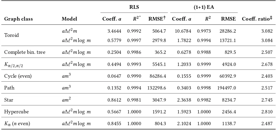
for hypercubes, butm∈ {1,2, . . . ,512}for, e. g., paths. For reasons of comparability and to keep the computational efort justiiable we take the values for the hypercube as the baseline and consider similar values for all other graph classes. For statistical soundness we perform50independent runs on each graph instance for both RLS and (1+1) EA and measure the number of function evaluations until a proper coloring withχ′(G)colors is generated for the irst time. Plots of the average running times of RLS5and itted regres-sion models with95%conidence intervals are depicted in Figure 3. Accompanying results of the regression analysis are provided in Table 2.6A visual inspection of the itted regression curves reveals that the models seem to it the data very well. This observation is supported by theR2indicator and the root mean squared error (RMSE). While the former measures the fraction of variation in the data explained by the model (the closer to 1 the better), the latter describes the average deviation of predicted values and actual observations from the data. TheR2values are≥0.99for all trained models, indicating a very good it. This is supported by the low RMSE values (relative to the potential range of itness evaluations for the corresponding graph class).
Moreover, we observe a clear pattern in the quotient of the estimated model coeicientsafor (1+1) EA and RLS which are all very close toe≈2.71. Sinceerelects the waiting time for (1+1) EA to perform a single local move, this suggests that (1+1) EA is most efective when only recoloring a single edge.
In summary, the experimental study supports all theoretical results obtained in this paper.
In all graphs studied here, the runtime was bounded by, or is conjectured to be bounded byO(∆ℓ2mlogm). (In some cases, such as cycles, paths, star graphs or potentially toroids, the logmfactor may be dropped.) The experiments gave further strong evidence for this bound for further graph classes, including hypercubes, complete graphs and complete bipartite graphs. In all cases we obtained a very good it with functionsa∆ℓ2mlogmora∆ℓ2mwith very reasonable leading constantsa. Again, the model suitability is supported byR2-values close to 1 and very low RMSE. In fact, in particular for complete bipartite graphs and all interesting special cases of bipartite graphs, i. e., toroids, complete binary trees and hypercubes, RMSE values are negligible and the model it is almost perfect. We hence state the following conjecture for future work.
Conjecture 26. RLS and (1+1) EA ind a proper∆-coloring for
every bipartite graphGwith maximum degree∆andℓ:=ℓ(G)in expected timeO(∆ℓ2mlogm).
8
CONCLUSIONS
We have presented the irst runtime analysis of evolutionary algo-rithms on the edge coloring problem, for which it isN P-hard to decide whether∆or∆+1 edge colors are suicient. We presented
general results on the time to obtain(2∆−1)-colorings, reducing the number of conlicts down tomand two lower bounds that apply
5We do not show plots for (1+1) EA since they do not reveal any more information. 6For regression analysis the statistical programming language R [23] (version 3.5.2)
Toroid
100 200 300 400
0e+00 2e+05 4e+05 m # f-e va lu a ti o n s
aΔl2m aΔl2mlog m
Complete binary tree
0 100 200 300 400 500
0 10000 20000 30000 m # f-e va lu a ti o n s
aΔl2mlog m
Complete bipartite
0 100 200 300 400 500
0e+00 2e+05 4e+05 6e+05 m # f-e va lu a ti o n s
aΔl2mlog m
Cycle (even)
0 100 200 300 400 500
0 2500000 5000000 7500000 m # f-e va lu a ti o n s am3 Path
0 100 200 300 400 500
0.0e+00 5.0e+06 1.0e+07 1.5e+07 m # f-e va lu a ti o n s am3 Star
0 100 200 300 400 500
0 50000 100000 150000 200000 250000 m # f-e va lu a ti o n s am2 Hypercube
0 100 200 300 400
0e+00 2e+05 4e+05 6e+05 m # f-e va lu a ti o n s
aΔl2mlog m
Complete (even n)
0 100 200 300 400 500
0e+00 5e+05 1e+06 m # f-e va lu a ti o n s
[image:13.612.58.557.84.331.2]aΔl2mlog m
Figure 3: Average runtime of RLS (black dots) and itted regression functions with95%conidence intervals separated by graph classes.
Table 2: Results of a regression analysis with diferent regression models for RLS and (1+1) EA for optimal edge-colorings on diferent graph classes.
RLS (1+1) EA
Graph class Model Coef.a R2* RMSE2 Coef.a R2 RMSE Coef. ratio3
a∆ℓ2m 3.4644 0.9992 5064.7 10.6784 0.9973 28286.2 3.082
Toroid
a∆ℓ2mlogm 0.5779 0.9997 2979.8 1.7822 0.9994 13721.1 3.084
Complete bin. tree a∆ℓ2mlogm 0.2504 0.9986 365.2 0.6278 0.9988 829.5 2.507
Kn/2,n/2 a∆ℓ2mlogm 0.4494 0.9993 5545.1 1.2033 0.9999 4924.0 2.678
Cycle (even) am3 0.0647 0.9990 86286.4 0.1555 0.9999 60392.9 2.403
Path am3 0.1352 0.9994 132298.6 0.3403 0.9998 194497.0 2.517
Star am2 0.8612 0.9981 3047.9 2.3638 0.9982 8234.7 2.745
Hypercube a∆ℓ2mlogm 0.5667 1.0000 1591.2 1.5923 1.0000 2456.4 2.810
Kn(neven) a∆ℓ2mlogm 0.8455 1.0000 804.3 2.1024 1.0000 1138.7 2.487
*R2: Fraction of variance explained by model;2RMSE: Root Mean Squared Error;3Quotient of regression coeicients of (1+1) EA and RLS
to all connected graphs. For cycles, paths, star graphs and arbitrary trees we have shown that simple evolutionary algorithms such as RLS and (1+1) EA are able to ind proper colorings with a minimum
number of∆colors eiciently, for all initial colorings (see Table 1 for details).
[image:13.612.74.533.415.630.2]