Two-to-One Resonant Multi-Modal Dynamics of Horizontal/Inclined Cables,
Part II: Internal Resonance Activation, Reduced-Order Models and
Nonlinear Normal Modes
Narakorn Srinil, Giuseppe Rega
Department of Structural and Geotechnical Engineering, University of Rome ‘La Sapienza’, via A. Gramsci 53, Rome 00197, Italy
Abstract. Resonant multi-modal dynamics due to planar 2:1 internal resonances in the non-linear, finite-amplitude, free vibrations of horizontal/inclined cables are parametrically investigated based on the second-order multiple scales solution in Part I [1]. The already validated kinematically non-condensed cable model accounts for the effects of both non-linear dynamic extensibility and system asymmetry due to inclined sagged configurations. Actual
activation of 2:1 resonances is discussed, enlightening on a remarkable qualitative difference of
horizontal/inclined cables as regards non-linear orthogonality properties of normal modes. Based on the analysis of modal contribution and solution convergence of various resonant cables, hints are obtained on proper reduced-order model selections from the asymptotic solution accounting for higher-order effects of quadratic nonlinearities. The dependence of resonant dynamics on coupled vibration amplitudes, and the significant effects of cable sag, inclination and extensibility on system non-linear behavior are highlighted, along with meaningful contributions of longitudinal dynamics. The spatio-temporal variation of non-linear dynamic configurations and dynamic tensions associated with 2:1 resonant non-linear normal modes is illustrated. Overall, the analytical predictions are validated by finite difference-based numerical investigations of the original partial-differential equations of motion.
1. Introduction
The goal of this paper is to parametrically investigate the multi-modal dynamics due to planar 2:1 internal resonances in the finite-amplitude free vibrations of horizontal/inclined cables based on the approximate closed-form solution obtained by the method of multiple scales (MMS) in Part I [1]. The underlying mechanical formulation is based on the kinematically non-condensed cable model accounting for the effects of both non-linear dynamic extensibility and system asymmetry due to inclined sagged configurations.
The suspended cable, aligned with the global Cartesian co-ordinate system, refers to Figure 1 in Part I [1], with an inclination angle θ assigned by keeping the horizontal span XH fixed and
varying the vertical span YH. The function y = y(x), where x is the spatially independent co-ordinate, describes the cable sagged static equilibrium, and the ensuing planar dynamics about it is described by the coupled longitudinal (horizontal) u and vertical v displacements. The dynamic behavior of horizontal/inclined cables is governed by several geometrical and mechanical parameters that can be collected in the unique parameter [2]
λ π =
( ) (
1π w SC cosθ)
2EA Ta3 , (1) which accounts for also the inclination θ effects, S being the cable equilibrium length, E the cable Young’s modulus, A its uniform cross-sectional area, wC its self-weight per unit unstretched length, and Ta the static tension at the cable point where the local inclination angle is approximately equal to θ. The input values of EA and wC are fixed for a given θ, whereas the cable static tension (or its horizontal component H) is adjusted to attain the varying λ⁄π, which entails varying values of Ta, S, and cable sag-to-span ratio d. Following [1], a low-extensible cable with a fixed parameter EA/wCXH≈ 2580.35 is analyzed for different θ values. Variation ofThe distinguishing linear dynamic features between horizontal and inclined cables are apparent from Figure 1, namely (i) the modification from crossover (Figure 1a) to avoidance or veering (Figure 1b) phenomenon, and (ii) the associated transition from purely symmetric/anti-symmetric modes to hybrid or asymmetric/anti-symmetric modes†. Amongst other planar (as well as non-planar) internal resonances, nearly tuned planar 2:1 resonances, each one involving the pair of modes (r,
s) indicated along a vertical dotted line, may occur away from (e.g., λ/π≈ 1.28, 2.95, 3.23 and 5.48) crossover/avoidance (λ/π ≈ 2nπ, n=1, 2,..), whereas nearly tuned planar 1:1 or 2:1 resonances may occur at each crossover/avoidance, involving also out-of-plane modes, thus leading to a multiple internal resonance [3]. Herein, we aim at characterizing the non-linear dynamic features of horizontal/inclined cables away from crossover/avoidance, which are more likely responsible for purely planar resonant dynamics – rarely investigated in the literature –, along with the combined effects of cable sag and inclination. Yet, near-avoidance inclined cables having high modal density will also be analyzed here in order to clarify the strong coupling role of the two coexisting hybrid modes and their significant contribution to system non-linear dynamics.
The paper is organized as follows. In Section 2, the actual activation of planar 2:1 internal resonances in various horizontal/inclined cables is investigated by taking into account the non-linear orthogonality properties of normal modes. The first-order interaction coefficients of different horizontal cable models are also discussed. Then, on accounting for second-order quadratic non-linear effects, a multi-dimensional, resonant/non-resonant, modal contribution analysis of the MMS solution is made in Section 3, and the solution convergence is evaluated in Section 4 in terms of resonantly coupled amplitudes and frequencies. Because the accurate determination of cable non-linear modal shapes is of primary interest from a practical point of view as regards long-term dynamic tension effects, the coupled dynamic configurations of
†
resonant non-linear normal modes (NNMs) are determined in Section 5, whereas Section 6 addresses the cable non-linear dynamic tension and its space-time modification. Overall results highlight significant effects of cable sag, inclination and extensibility on system non-linear dynamics. Numerical time histories of the finite difference-based solution, validating the analytical predictions and showing modal interaction features of the original system, are presented in Section 7. The paper ends with a summary and some conclusions. Throughout the paper, reference to Part I [1] is made, where needed, by labeling the relevant Section, Figure, Table and Equation number with the preceding roman ‘I’ symbol.
2. Internal Resonance Activation
Actual activation (non-activation) of planar 2:1 resonance involving a high-frequency (s) and low-frequency (r) mode is governed by the first-order quadratic coefficient ℜ obtained by the MMS, when it is different from (equal to) zero [4]. Based on the kinematically non-condensed model holding for a generic inclined cable, it reads [1]
1 3 0
3 1 3
2 ,
2 2 2 2
s r r r r r r s r r r r r r
y
y y dx
α φ φ φ φ ϕ ϕ ϕ ϕ φ φ φ ϕ ϕ ϕ
ρ
′
′ ′ ′ ′ ′ ′ ′ ′ ′ ′ ′ ′ ′ ′ ′ ′
ℜ = − + + + + +
∫
(2)where a prime denotes differentiation with respect to x, ρ= 1+y′2 , = EA/H, φm and ϕm are the longitudinal and vertical shape functions of the m(m = r, s) planar mode obtained by the Galerkin method using a properly truncated N sine-based series, see Section I.2.4. To discuss also the strain condensation effects on the resonance activation, we evaluate ℜ with the condensed model of horizontal cable as well,
1 1 1 1
0 0 0 0
1
2 ,
2
s rdx y rdx sy dx r rdx
α ϕ ϕ ′′ ′ ′ϕ ϕ ′′ ϕ ϕ′ ′
ℜ = +
∫
∫
∫
∫
(3)whose ϕm are available in closed form, see Appendix I.A. The ℜ value in Equations (2) and (3)
2.1 Horizontal Cables
Previous analytical [4] and numerical [5] investigations have shown that a planar 2:1 internal resonance in horizontal cables is not activated when the high-frequency mode is anti-symmetric, even though a 2:1 (ωs:ωr) frequency ratio is satisfied. Such circumstance is herein ensured in
Table 1 by the vanishing of ℜ coefficients of both the non-condensed (NC) and condensed (CC) crossover cables (λ/π ≈ 2, 4) because of the non-linear orthogonality properties of the anti-symmetric/symmetric (high/low -frequency) modes. On the other hand, due to the involvement of just symmetric high-frequency s modes for non-crossover (λ/π ≈ 1.28, 2.95, 3.23, 5.48) and crossover (λ/π ≈ 4) cables (Figure 1a) having different geometrical (d) and mechanical (α) properties, the 2:1 resonances are activated for both NC and CC models (ℜ ≠0), regardless of the low-frequency r modes being symmetric or anti-symmetric.
To highlight also the ρ-term effects – already addressed through numerical studies in Section I.5.3 – on the ℜ values of the resonantly activated cables, two NC cases, i.e., with ρ≠ 1 and ρ≈ 1, are considered. It can be seen that the ℜ values of the NC (ρ≈ 1) and CC models are slightly different from each other, whereas the latter differ more significantly from those obtained with the general NC (ρ≠ 1) model, notwithstanding the corresponding sag d values are small for all considered cables (i.e., d < 1:8, see [6]).
contributions affects the resonance activation only slightly through the ℜ values appearing at the first-order MMS. However, when continuing the MMS analysis to second order, the discrepancies in the quadratic and, especially, cubic coefficients between NC and CC models become outstanding due to the different combination of coupled quadratic/cubic-based coefficients governing various resonant/non-resonant modes (see Table I.3 and Section I.5.4). As a consequence, greater differences may occur. It is also important to remark that the kinematic condensation plays a more pronounced role when considering a larger-sagged or higher-extensible resonant cable [1].
In Figure 2, we show the negligible difference in the ϕm modal shape functions of the NC and CC models through the normalized vertical configurations (vn) of the symmetric 2nd (r = 2) and
5th (s = 5) modes of the cables with λ/π≈ 2.95 (Figures 2a, 2b) and 5.48 (Figures 2c, 2d). Solid (dotted) lines represent NC (CC) results. It is worth noting that, in spite of the apparent opposite phase occurring in ϕr between the two models for λ/π ≈ 5.48 (Figure 2c), there is no sign difference in the associated ℜ values in Table 1. This is because the r-mode enters Equations (2) and (3) in couple, so that they are independent of the relevant phase change. In contrast, if the phases of the solely-appearing s-mode of the two models are opposite to each other, a sign difference is expected, which, in turn, could affect the resonant NNMs (Equations I.41-I.45) for given system parameters. Yet, such opposite phase does not affect the sign of second-order quadratic coefficients as the latter, embedded in Equations (I.33)-(I.35), appear in couple.
Section I.5.3 has shown how the non-linear planar responses of the approximate NC model with ρ ≈ 1 exhibit greater numerical errors, with respect to the exact model, than those of the corresponding NC model with ρ ≠ 1. Moreover, Table 1 exhibits different ℜ values of various NC or CC models, whose differences become much stronger at second order (see, e.g., Table I.3). Accordingly, in order to achieve the most reliable analytical results, the following parametric studies, which are based on the second-order MMS, will rely upon the NC model, with the pertinent non-linear coefficients accounting for the contribution of longitudinal dynamics (no strain condensation) and ρ ≠ 1,. In turn, some results based on ρ ≈ 1 of the NC model are reported in [7, 8].
2.2 Inclined Cables
Consider now inclined cables with the general NC model. The 2:1 resonance activation, with
0
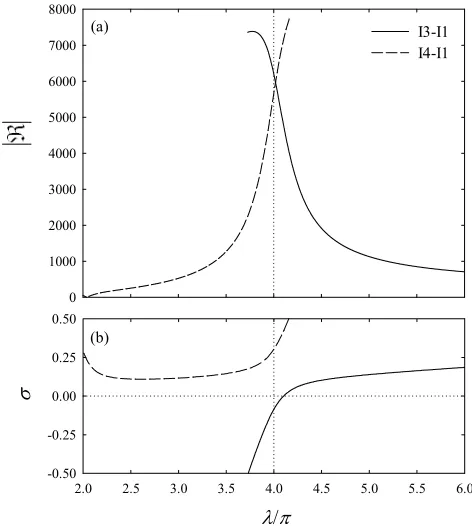
ℜ ≠ , is nearly always possible in the frequency spectrum (Figure 1b), due to vanishing of the purely symmetric or anti-symmetric spatial character of one of the two (or both) involved modes as a consequence of the asymmetry effects due to inclined sagged configurations. In other words, the non-linear orthogonality properties of normal modes never hold. As an example, the 2:1 resonance involving the high-frequency (asymmetric or hybrid) third (I3) or fourth (I4) mode and the low-frequency first (I1) mode may be activated near second avoidance (λ/π≈ 4), besides those of non-avoidance cables having the same λ/π as non-crossover cables (1.28, 2.95, 3.23, 5.48). This is shown in Figures 3a and 3b by the variation versus λ/π of the ℜparameters and of the frequency-tuning σ effects, respectively, for the cable with θ = 30o and N = 15.
despite the non-vanishingℜ. Indeed, being σ significantly different from zero, the frequencies may be far away from proper tuning, consider, e.g., the high values of bothℜ ≈ 7729 (7360) and σ ≈ .5 (-.5) at λ/π≈ 4.16 (3.73) for the I4-I1 (I3-I1) interaction. This implies that ℜ≠ 0 is a necessary, but not sufficient, condition for such internal resonance to be activated, and that the σ value has also to be accounted for. Regardless of the latter, it is worth noting that the two I3-I1 and I4-I1 interactions involving the same I1 mode yield almost equal values ofℜ(≈ 5964.018 and 5967.215) at λ/π ≈ 4.019, thus showing the negligible effect of the difference in hybrid shape functions associated with the two coexisting avoidance modes (I3, I4) on theℜvalue. However, this effect increases as λ/π is far away from avoidance.
In contrast with near-avoidance cables, theℜvalues of the I3-I1, I4-I1 interactions progressively decrease – due to decreasing level of “modal hybridity” – as λ/π moves towards the right (λ/π → ∞) or left (λ/π →2) of second avoidance, respectively, which ultimately reflects the occurrence of a nearly anti-symmetric high-frequency mode.
Overall, the outcomes of the nearly tuned 2:1 resonance activated at second avoidance, irrespective of the involved high-frequency, hybrid, 3rd or 4th mode, theoretically confirm the numerical results in [9], and enlighten on the distinguishing dynamic behaviors of the second-avoidance cable with respect to those of the second-crossover cable, whose 2:1 resonance is activated only when the high-frequency mode, out of the two coexisting modes, is symmetric [5]. As a general remark, the present analysis gives broad hints about the most likely involvement of a larger number of modes within a multiple internal resonance for avoidance than for crossover cables [e.g., 10, 11], owing to the non-satisfied non-linear orthogonality of the relevant modes.
Some resonant non-avoidance (λ/π≈ 1.28, 2.95, 3.23, 5.48) and near-avoidance (λ/π≈ 3.84, 4.14) inclined cables are given in Table 2, with their properties (θ, d, α, ωr, ωs) and ℜ values (N
non-crossover cables, those of all non-avoidance cables (θ = 30o) decrease, even though both the sag d and α parameters substantially increase. This is likely due to the role played by the inclination θ, which, in fact, significantly alters the relative importance of the longitudinal and vertical shape functions affecting the ℜ value. Accordingly, this further decreases as θ becomes 45o and 60o for λ/π ≈ 2.95, consistent with the increasing (absolute) value of σ (≈ -.02, -.10, -.24) as θ = 30o, 45o, 60o, respectively, which shifts the system dynamics far away from nearly-perfect tuning. Indeed, as displayed in Figure 4, though involving the same resonant modes (r = 2, s = 5) for all θ, the (normalized) un plays an increasing role with respect to the corresponding
vn in both the low- (4a, 4c) and high-frequency (4b, 4d) modes as θ increases, up to becoming the most significant component. This shows how the cable inclination plays a role in linear dynamics not only as regards the occurrence of asymmetric modes at avoidance, and generally affects the non-linear dynamics up to giving the smallest ℜ value for the maximum θ (60o).
3. Resonant/Non-Resonant Quadratic Modal Contributions
Apart from the first-order quadratic coefficient ℜ governing resonance activation, the second-order MMS solution of the coupled amplitudes and frequencies also depend on the second-order coefficients Krr, Kss, and Krs (Equations (I.33)-(I.35)), which account for the
combined effects of quadratic/cubic contributions due to the two resonant (modeled) modes, and for the solely quadratic contributions due to the non-resonant (non-modeled) modes. Thus, prior to evaluating the non-linear dynamic displacement and tension profiles, which are amplitude- and frequency-dependent, it is deemed necessary to examine the quadratic modal contributions responsible for solution convergence. Accordingly, the pertinent percent contributions to each of the quadratic coefficients (labeled ΚQii, i = r, s) are evaluated by considering a finite-dimensional model through which M is the highest order of retained modes.
the cable sag effects. In each λ/πcase, the results for θ = 0o (Table 1) and 30o (Table 2) are comparatively reported to show the influence of cable inclination. It can be seen that only the non-resonant symmetric modes contribute to all coefficients for horizontal (non-crossover) cables [5, 12], whereas all non-resonant modes – regardless of their order or spatial character – come into play for inclined cables. This distinctive aspect also holds for the second-order spatial functions of dynamic displacement and velocity (Equations (I.51)-(I.52)). For the cables with
λ/π ≈ 1.28, the quadratic effects due to non-resonant modes, which, in general, can be either positive (softening-type correction) or negative (hardening-type correction), are very small compared with those produced by the two resonant modes (> 99 %). Therefore, for these cables, it makes sense to consider a two-degree-of-freedom reduced-order model accounting for only the two resonant modes. However, this is not the case for the larger-sagged cables with λ/π ≈ 5.48, for which the higher-order effects of quadratic nonlinearities become pronounced. As shown in Table 4, a number of non-resonant modes, e.g., the intermediate-order 4th (3rd and 4th) and the higher-order 7th, 9th, 11th (6th, 7th, 9th and 11th) modes play a meaningful role, too, in all quadratic coefficients of the horizontal (inclined) cable.
In other cases, some non-resonant modes are seen to play a role even greater than the resonant ones. This may happen, for instance, when the associated λ/π values fall in the avoidance zones (Figure 1b), where multiple internal resonances are realized. Consider, e.g., the resonant inclined (θ=30o) cable in Table 2 involving the coupled 1st and 4th modes or the coupled 1st and 3rd modes, whose λ/π is nearly below (λ/π ≈ 3.84) or above (λ/π ≈ 4.14) second avoidance, respectively. As shown in Table 5 with M = 15, the combinations (103.514 %, 94.865
%) of non-resonant modal contributions in the ΚQrr are greater than those (-3.514 %, 5.135 %) of
resonant modal contributions for both λ/π (3.84, 4.14), whereas, in the ΚQrs, the former may be greater than (65.832 %) or nearly equal to (44.038 %) the latter (34.168 % or 55.962 %) for
from the contribution of the 3rd (4th) hybrid mode which nearly coexists with the 4th (3rd) one near avoidance at λ/π ≈ 3.84 (λ/π ≈ 4.14). Yet, other non-resonant modes, e.g., the intermediate-order 2nd and the higher-order 5th modes also play a significant role for both λ/π, like those in Table 4 for cables with λ/π ≈ 5.48.
In conjunction with Equations (I.33)-(I.35), these meaningful contributions are due to the associated nearly-vanishing denominators where the difference between squared resonant and non-resonant frequencies appears, as well as to the coupled quadratic terms whose values are non-trivially affected by the asymmetric spatial character of the coexisting hybrid modes. The former are responsible for a multiple resonance condition of near-avoidance cables. Overall, the quadratic modal contributions put into evidence the significance of accounting for both resonant and non-resonant (higher-order) modes in the resonant dynamic solution of cables exhibiting significant sag and/or remarkable asymmetry due to inclination effects. Of course, the higher-order modal contributions become less important when increasing the higher-order of modal truncation up to finally yielding converging results. It is also worth noticing how the resonant two-mode solution, when embedded in an infinite-dimensional Galerkin expansion, is capable of properly signaling the breakdown of the lowest reduced-order modeling. Thus, accounting for also non-resonant modes becomes mandatory.
4. Resonant Non-linear Amplitudes and Frequencies
are comparatively displayed in Figures 5a, 5b and 5c for λ/π≈ 1.28 (r = 1, s = 3), λ/π≈ 2.95 (r = 2, s = 5) and λ/π≈ 4.14 (r = 1, s = 3), respectively. For the sake of comparison, fixed σ = 0 and γ = π values are considered, and only stable positive amplitudes according to Equation (I.42) are presented.
Figures 5a and 5b highlight that considering only the first-order term gives considerably overestimated ar versus as values with respect to those obtained by second-order solutions. For the low-sagged cable (λ/π ≈ 1.28), the second-order amplitude curves, obtained with M = R
(accounting for only the two resonant modes), M = 3 (confirming the no-contribution of the anti-symmetric 2nd mode) or M = 5 in Figure 5a, are nearly undistinguishable from each other. Thus, it is definitely reasonable to consider only the minimal (2-DOF) reduced-order resonant model for this cable, because the quadratic effects due to non-resonant modes are negligible. However, as the cable sag increases (Figure 5b, λ/π≈ 2.95), considering only the resonant modes (M = R) in the second-order solution entails underestimated ar values which, in addition, are limited to a low amplitude as range, due to the rapidly approaching negative value of the resulting term in the
bracket of Equation (I.41). The solutions improve and converge at once when considering M = 5. This means that, since there is no contribution from the anti-symmetric 1st and 4th modes (see Figure 1a), accounting for only the intermediate symmetric 3rd mode is already satisfactory. Of course, in other λ/π ≈ 2.95 cases with θ ≠0, the 1st and 4th modal contributions are non-trivial. Depending on the symmetric modal interaction, it is also observed that the obtained ar
amplitudes decrease as the sag or λ/π increases for the fixed θ and given as amplitudes.
Unlike horizontal cables, the asymmetry effects play a significant role for the near-avoidance cable shown in Figure 5c. The first-order and M = R second-order solutions yield almost the same ar values, which remain unchanged even if accounting for also the 2nd mode (M = 3). When
range. Eventually, the results converge when M = 5, confirming the need to consider also some non-resonant higher-order modes in Table 5.
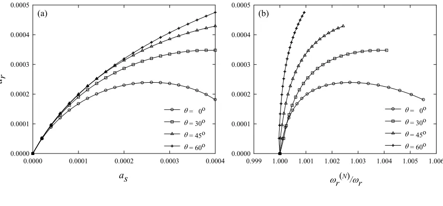
The effects of varying θ on both the ar-as relationship and the backbone curve are now displayed in Figures 6a and 6b, respectively. Since ωs(N) ≈2ωr(N) [1], only the r-mode non-linear frequency (ωr(N)) is evaluated through Equation (I.45) and then normalized with respect to the associated linear frequency ωr. With λ/π ≈ 2.95, the second-order results are shown for the horizontal and inclined (θ = 30o, 45o 60o) cables with M = 5 and 10, respectively. In view of Figure 6a, the estimated ar amplitudes increase as θ (as well as the cable sag) increases for given as values, contrary to the case exhibiting the increased sag effects alone (Figures 5b vs 5a). This may be due to exchanged importance of the u/v shape functions (Figure 4) as θ increases, according to which the u component becomes the dominant contribution to cable response and gives rise to significant changes in the associated non-linear coefficients (ℜ, Krr, Kss, Krs). As
shown in Table 6, the inclination affects both the second-order quadratic (ΚQii ) and cubic (ΚCii) coefficients, which are of softening-type and hardening-type, respectively. As θ increases, all of the absolute summations (∑) of quadratic and cubic coefficients decrease, without changing the sign indicating the effective nonlinearity. Evidently, together with the ℜ decrement in Table 2, this entails an overall increment of the estimated ar values through Equation (I.41), while
keeping σand γ fixed. Thus, while the backbone curves in Figure 6b exhibit, in general, a hardening behaviour, they become as less hardening as higher θ is. This occurs because, as θ increases, the softening correction due to the ar-dependent term in Equation (I.45) somehow reduces the prevailing hardening corrections due to the first-order (remind that ℜ is positive, while cosγ is negative) and as–dependent terms. This augmented softening behaviour appears consistent with the effects of the solely increased sag in non-resonant horizontal cables [3].
horizontal cables with λ/π≈ 2.95 (N = 30, M = 5). While keeping A, wC and XH fixed, the E value (extensibility) is increased (decreased) such that EA/wCXH ≈ 10000, 20000 with respect to the reference one (2580.35). Meanwhile, in order to maintain λ/π≈ 2.95 in Figure 1a, the H and Ta
(sag) values increase (decreases) as E increases. The assumption of small static strain [1] is still satisfied, and the second-order contributions from the non-resonant 3rd mode remain significant. In addition, the absolute values of first-order – as well as second-order (ℜ and Krr remain
positive, while Kss and Krs remain negative) – coefficients decrease as EA/wCXH decreases, even
though the sag increases. Because of the slight changes in the modal shape functions of low-extensible cables, this decrement is mainly due to the decrement of the pertinent
α (=ΕΑ/Η) parameter, despite H also decreases. Similar to the increasing θ case, the estimated
ar values increase as the extensibility increases for given as, as shown in Figure 7a. This is a physically expected behaviour because a lower-extensible (e.g., metallic) cable vibrates with smaller amplitudes than a corresponding higher-extensible (e.g., synthetic) cable. Accordingly, the backbone curve in Figure 7b exhibits as more hardening behaviour as lower the extensibility is: this is again expected as the metallic cable is typically stiffer than the synthetic cable. The
σ and γ parameter effects on the amplitude/frequency results can be found in [7].
5. Resonant NNMs and Their Space-Time Evolution
The second-order effects on the spatial dynamic configurations of the 2:1 resonant NNMs are now illustrated. Three different cables are analyzed in Figures 8a, 8b and 8c, respectively, i.e. the horizontal cable with λ/π ≈ 2.95 and as = .0002 (Table 1), and the inclined (θ = 30o) cables (Table 2) far away from avoidances (λ/π ≈ 5.48, as = .0015) or near second avoidance (λ/π ≈ 4.14, as = .0003). To gain clear insights into different MMS solutions, the first-order, improved
first-order and second-order dynamic configurations (see their definitions in Section I.4.3) of the
v amplitudes (with 51 cable nodes) are comparatively presented with γ = π, σ = βr0 = t = 0, the
Overall, it can be seen that significant quantitative (Figures 8a-8c) as well as qualitative (8b and 8c) errors occur when considering the first-order configurations, due to the overestimated (or underestimated) ar amplitudes at first order, e.g., in Figures 5a and 5b (or 5c). Thus, it is very
important to account for second-order corrections – depending on the non-resonant modes – in both the amplitudes and frequencies. In Figure 8a, quantitative errors are seen to occur also if considering M = R in the second-order displacement. The results suggest taking the symmetric 3rd mode (M = 5) into account, consistent with the observation in Figure 5b, the 7th mode (M = 7) being instead useless. Yet, it is worth noticing how only a small difference occurs between the improved first-order and the second-order configurations with M = 5, which fully highlights the major importance of accounting for higher-order effects in the amplitude and frequency even in a first-order displacement solution, in order to achieve a reliable NNM. This spatial convergence property also holds when varying the time t.
In contrast, the importance of accounting for the full second-order analysis (involving also spatial corrections) is apparent in Figures 8b and 8c which refer to the larger-sagged and inclined cables, whose asymmetric features of all superimposed configurations are clearly noticed with respect to the symmetric horizontal cable in Figure 8a. In agreement with Tables 4 and 5, the spatial configurations converge satisfactorily when considering the second-order displacement solution accounting for both resonant/non-resonant modes (e.g., M≈ 7 in Figure 8b and M≈ 5 in Figure 8c), whereas the improved first-order solution does not converge albeit considering more modes (M = 15 in Figure 8b and M = 11 in Figure 8c). This makes evident that the second-order quadratic nonlinearities are significant for larger-sagged and asymmetric cables, and gives clear hints about the necessity of accounting for also second-order spatial displacement corrections.
frequency solutions only, thereby developing an improved first-order displacement solution, for relatively low-sagged cables; (iii) it is necessary to take them into consideration also in the non-linear dynamic displacements (the second-order spatial solution) as the cable sag or inclination effects are significant.
The space-time evolution of the second-order displacements of resonant NNMs is addressed by referring to both the u (dashed lines) and v (solid lines) components in the analysis over a half non-dimensional r-mode period Tr of non-linear oscillation. They are shown in Figures 9a, 9b and 9c, with M = 5, 10 and 15, respectively, for the horizontal and inclined (θ = 45o) cables with
λ/π ≈ 2.95, as = .0004, and for the inclined (θ = 30o) cable with λ/π ≈ 5.48, as = .001. Having in mind the u and v modal shapes of the underlying 2nd and 5th resonant modes for the horizontal and inclined (θ = 45o) cables in Figure 4, an apparently distinctive time-varying non-linear superposition of the two coupled modes is observable in Figures 9a and 9b. Qualitatively, as θ increases, the longitudinal amplitudes – which are quite small for the horizontal cable – meaningfully increase, up to becoming comparable with the combined vertical ones, which, in turn, are relatively lower than in the horizontal cable. This visualizes how the longitudinal displacements play an increasingly important role in the non-linear resonant dynamics as θ increases for a fixed λ/π, and represents a closed-form confirmation of a behavior already exemplified in [9] within a purely numerical solution. Furthermore, a remarkably different time evolution is observed between the symmetric/asymmetric spatial distributions exhibited by the horizontal/inclined cables, respectively.
6. Space-Time Modification of Cable Non-Linear Tensions
On accounting for the spatial variation of both static e and non-linear dynamic ed strains, the space-time modification of cable total tension can be evaluated through Equation (I.5) with neglected out-of-plane component, wherein the derivatives of the converging second-order u and
v displacements are calculated through Equation (I.43). Tf is the linear total tension
non-dimensionalized with respect to the maximum static tension, which typically takes place at the left support (both supports) for the inclined (horizontal) cable (Figure I.1). Two interesting aspects are emphasized: (i) the inclination effects on the spatial distribution of Tf response
shown in Figure 10a (for cables with λ/π ≈ 2.95, as = .0004 and t = .3Tr); (ii) the space-time Tf
distribution exhibiting the strain variation effects shown in Figure 10b (for the inclined cable with θ = 30o, λ/π ≈ 5.48, as = .001, t = 0-.5Tr). Again, the prescribed values γ = π, σ = βr0 = 0 are
assigned in all cases.
Figure 10a clearly shows that, while the spatially symmetric Tf response of the horizontal cable exhibits a limited variation along the cable span-length, the spatially unsymmetrical Tf
responses of all inclined cables (see also Figure 9b for θ = 45o) markedly diminish (non-linearly) as one moves towards the right support or as θ increases. This entails a meaningful difference between the maximum/minimum total tensions, which increases with θ [9], and implies that, during non-linear vibrations, the resulting total tension at any cable point is smaller than the initial maximum static tension due to a negative oscillation-induced tension. Accordingly, the non-linearity produces a less-hardening behavior of higher-inclined cables, as already observed in Figure 6b. From the engineering viewpoint, special care has to be paid to the possibility of cable loosening [13] at the lower-right end support as θ increases (see, e.g., Figure 10a, θ = 60o), this being one major design aspect. Yet, also the maximum Tf taking place at the left-end support
considerably greater or smaller than their initial estimated values, with the left-support tension still exhibiting the maximum value, whereas the mid-span tension exhibiting the minimum one. Consequently, the time-varying difference between maximum/minimum tensions becomes appreciable at a specific time, highlighting that the usual strain condensation model assuming spatially-uniform dynamic tension is no more suitable for such small-sagged cable exhibiting internal resonance.
In Figure 10b, the overall space-time variability of tension response becomes even more apparent for the inclined and larger-sagged cable, where the spatially uniform and non-symmetric features are seen to entail the occurrence of the largest or smallest values of total tension along time evolution, also at cable positions other than the supports: see, e.g., the distributed tension peaks occurring at t = 0 or .5Tr, and their associated configurations in Figure
9c. All of these results confirm the advantage of making use of the non-condensed model which properly accounts for the spatial variability of non-linear dynamic strain, in order to ascertain the actual extreme values of total tension response.
7. Modal Interaction Features: Numerical Validation of Analytical Predictions
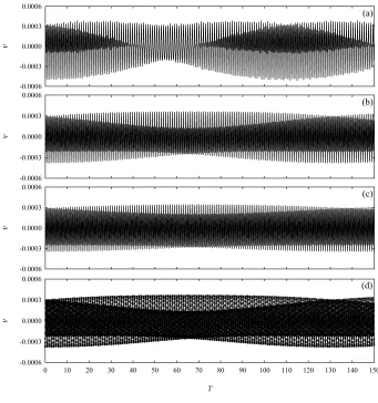
The analytical MMS predictions are now validated by numerical results. Instead of integrating the system ODEs (I.17) with a prescribed number of modes, the space-time finite difference method (FDM), coupled with a predictor-corrector iteration [5, 7], is directly applied to the original PDEs (I.53-I.54) neglecting the out-of-plane component, to determine the actual dynamic responses under specified initial conditions. To this end, the responses are initiated by the associated coupled displacements (Equation I.43) and velocities (Equation I.44). In the following, the non-dimensionalized responses are plotted against the time parameter T obtained by non-dimensionalizing the physical time with respect to the r-mode natural period.
obtained with the u, v initial displacement conditions of first-order, improved first-order and second-order configurations are comparatively illustrated in Figure 12. Depending on the obtained ar amplitudes for the specified as = .0002 (Figure 5b), it can be seen that all responses
show the periodically-modulated interaction features due to the 2:1 resonance, but some of them differ in both the extent and duration of the modulation, see the first-order (Figure 12a), improved first-order with M = 5 (Figure 12b) and second-order with M = R (Figure 12c) time histories. Yet, the modulation feature in the response initiated by the improved first-order solution (Figure 12b) is practically similar to those in the responses initiated by the second-order solutions with M = 5 (solid lines) or 10 (circles) in Figure 12d. This highlights, with regard to the temporal aspect, both the possibility of considering just the improved first-order solution and the convergence properties of the second-order spatial solution, already observed in the analytical framework. This holds also for the corresponding inclined cable which exhibits equally comparable FDM time laws as the present horizontal cable [8]. Of course, the amplitude modulations characterizing the actual resonant interaction in Figure 12 initiated by the coupled-mode displacements are substantially different from those initiated by the single-coupled-mode ones in Figure I.7. On the other hand, they do not occur in the periodic time laws corresponding to the stationary amplitude MMS solutions.
Moving to various inclined cables with λ/π ≈ 2.95 and larger as = .0004 (corresponding to Figure 6), meaningful differences in terms of extent and duration of resonant modal interactions are noticeable in the u (solid lines) and v (dashed lines) responses at 1/8 span shown in Figure 13, which are initiated with the second-order u and v displacements at t = 0. With respect to Figure 12d for the horizontal cable with as = .0002 and ar ≈ .00023 (Figure 6a), the horizontal
cable response in Figure 13a has a longer modulation due to the relatively different contribution of the lower ar ≈ .00018: this reflects the amplitude-dependence of system resonant dynamics
60o (Figure 13d) exhibits the shortest modulation. This highlights the inclination effects on the non-linear temporal features of the original system. The Fourier amplitude spectral densities (PSDs) of the v responses in Figure 13 are also reported in Figure 14, all of them clearly revealing two major frequencies. This property and the observed beating-type energy transfer due to modal interaction confirm the theoretical prediction about activation of the planar 2:1 resonance involving just the modeled 2nd and 5th modes of non-crossover/non-avoidance cables.
With the second-order MMS initial displacement conditions at t = 0, the numerical FDM v
responses (at node 6) showing the effects of varying the given as amplitude, or the angle θ, or the extensibility E on the response of cables with λ/π ≈ 2.95 are summarized in Figures 15a-15c, respectively, also to the aim of validating the non-linear behaviors predicted by the MMS solution. For a fixed θ, i.e. for the horizontal cable, Figure 15a shows that (i) the system responses are as more hardening as greater as is, in agreement with Figure 6. In turn, when varying the angle θ for a fixed as =.0004, (ii) the responses in Figure 15b reflect the less-hardening non-linearity as θ increases, again in agreement with Figure 6. Moreover, when varying the extensibility for fixed θ = 0o and as =.0002 values, (iii) the response in Figure 15c is seen to be as more hardening as higher the parameter EA/WCXH is, in agreement with Figure 7. Hence, overall analytical predictions are validated by numerical FDM results.
Next, it is interesting to evaluate how the non-linear resonant response evolves when initiating both the spatial displacement and velocity fields of second-order MMS solution, with respect to that initiated by zero-velocity (t = 0) displacements. For this purpose, two initial u, v
conditions are considered: one corresponding to the MMS displacements at t = 0; the other corresponding to the MMS displacements/velocities at t = .3Tr. The associated FDM u responses
behavior in both figures regarding the extent and duration of the resonantly periodic modulation, which, indeed, holds true also for other inclined cables. Thus, the characterizing amplitude-modulated response of the original system is shown to be invariant with respect to the stationary MMS displacements and/or velocities entering the initial conditions. In addition, the numerical results confirm that, apart from the distinctive extent of modulation, the duration of modal interaction is the same at different cable positions.
Finally, the amplitude modulation features of the non-dimensional FDM-based displacement and velocity are illustrated through the phase portraits in Figures 17a (1/8 span), 17b (1/4 span) and 17c (mid-span) against the corresponding stationary MMS-based portraits in Figures 17d, 17e and 17f, respectively, for the horizontal cable with λ/π ≈ 2.95 and as = .0002 under initial
conditions of the second-order MMS at t = .3Tr. Besides confirming the different extent of
amplitude modulation occurring at different cable positions, the overall similarity between non-stationary (FDM) and non-stationary (MMS) phase portraits is highlighted, with the mid-span response exhibiting the largest portrait and modulation.
8. Summary and Conclusions
Based on the kinematically non-condensed cable model accounting for the effects of both non-linear dynamic extensibility and system asymmetry due to inclined sagged configurations, planar 2:1 resonant multi-modal non-linear free vibrations of horizontal/inclined cables have been investigated through the second-order multiple scales solution obtained in Part I [1]. The main features of the parametric analysis are summarized as follows.
in inclined cables is nearly always possible – depending on frequency-tuning and hybridity capacity – and occurs over a wide range of system parameters.
(ii) Based on a multi-dimensional Galerkin discretization, analysis of second-order quadratic modal contributions has shown that, besides the two resonant modes, only symmetric non-resonant modes affect the solution of (non-crossover) horizontal cables, whereas all non-resonant modes – irrespective of their order or spatial character – do contribute for inclined cables. Moreover, some non-resonant modes may play a role even greater than the resonant ones. This occurs, for instance, in the avoidance zone of the frequency spectrum wherein, due to the system high modal density and strong coupling, the non-modeled hybrid mode – out of the two coexisting at avoidance – contributes to the response greater than the directly-modeled hybrid mode. This highlights the necessity of accounting for both of them and the possible involvement of a larger number of coupled modes in avoidance cables than in crossover cables.
(iii) As regards the reduced-order modeling issue, the convergence studies accounting for higher-order effects of quadratic nonlinearities on non-linear amplitudes, frequencies and dynamic configurations of the resonant NNMs have indicated that, depending on the system parameters and coupled amplitudes, the contributions of non-resonant (higher-order) modes are very important. The minimal (two-degree-of-freedom) model involving only the resonant modes shows capable of providing reliable results only for a very low-sagged cable. In turn, it may be sufficient to account for non-resonant modes in the non-linear amplitudes and frequencies only, thereby developing an improved first-order solution, for relatively low-sagged cables; otherwise, they should be accounted for also in the dynamic displacements (the full second-order solution) as the cable sag and/or inclination (asymmetry) becomes significant.
inclination increases, and the multi-harmonic response features owed to higher-order non-resonant modes for inclined sagged cables.
(v) The spatio-temporal variability of non-linear dynamic tension has been presented, emphasizing the importance of accounting for spatial variation of cable non-linear strain through the non-condensed model since appreciable time-varying differences between maximum/minimum total tensions occur even in shallow horizontal cables.
Overall, significant effects of cable sag, inclination, extensibility as well as longitudinal displacements on the non-linear resonant dynamics have been evidenced. Moreover, finite
difference displacement time laws obtained from the original partial-differential equations of
motion have confirmed the predictions and the amplitude-dependent properties of the multiple
scales solution, by also showing periodically modulated interaction features.
Apart from making available the approximate general non-condensed model valid for horizontal/inclined sagged cables, and for showing its thorough accuracy with respect to the exact model in Part I [1], the comprehensive analysis of resonant non-linear normal modes has provided worthwhile information as regards deriving accurate reduced-order cable models and qualifying the non-linear dynamic properties of horizontal/inclined cables to be properly recognized within an upcoming forced vibration analysis.
Acknowledgements
Dr. Narakorn Srinil would like to express his gratitude to the support of the University of Rome ‘La Sapienza’, Italy, through a Postdoctoral Research Fellowship.
References
1. Srinil, N., Rega, G., and S. Chucheepsakul, ‘Two-to-one resonant multi-modal dynamics of horizontal/inclined cables. Part I: Theoretical formulation and model validation’, Nonlinear
2. Triantafyllou, M. S., and Grinfogel, L., ‘Natural frequencies and modes of inclined cables’,
ASCE Journal of Structural Engineering112, 1986, 139-148.
3. Rega, G., ‘Nonlinear dynamics of suspended cables. Part II: Deterministic phenomena’,
ASME Applied Mechanics Reviews57, 2004, 479-514.
4. Lacarbonara, W., and Rega, G., ‘Resonant nonlinear normal modes. Part II: Activation/orthogonality conditions for shallow structural systems’, International Journal of
Non-linear Mechanics38, 2003, 873-887.
5. Srinil, N., Rega, G. and Chucheepsakul, S., ‘Three-dimensional nonlinear coupling and dynamic tension in the large amplitude free vibrations of arbitrarily sagged cables’, Journal of
Sound and Vibration269, 2004, 823-852.
6. Irvine, H. M., and Caughey, T. K., ‘The linear theory of free vibrations of a suspended cable’, Proceeding of the Royal Society of London Series A341, 1974, 229-315.
7. Srinil, N., ‘Large-amplitude three-dimensional dynamic analysis of arbitrarily inclined sagged extensible cables’, Ph.D. Dissertation, King Mongkut’s University of Technology Thonburi, Bangkok, Thailand, 2004.
8. Rega, G., Srinil, N., and S. Chucheepsakul, ‘Internally resonant nonlinear free vibrations of horizontal/inclined sagged cables’, in Proceeding of the 5th International Conference on
Multibody Systems, Nonlinear Dynamics, and Control, California, USA, DETC2005-84752,
2005.
9. Srinil, N., Rega, G., and Chucheepsakul, S., ‘Large amplitude three-dimensional free vibrations of inclined sagged elastic cables’, Nonlinear Dynamics33, 2003, 129-154.
10. Rega, G., Lacarbonara, W., Nayfeh, A. H., and Chin, C. M., ‘Multiple resonances in suspended cables: Direct versus reduced-order models’, International Journal of Non-linear
Mechanics34, 1999, 901-924.
12. Arafat, H. N., and Nayfeh, A. H., ‘Non-linear responses of suspended cables to primary resonance excitations’, Journal of Sound and Vibration266, 2003, 325-354.
13. Wu, Q., Takahashi, K., and Nakamura, S., ‘Non-linear vibrations of cables considering loosening’, Journal of Sound and Vibration261, 2003, 385-402.
List of Figures
Figure Page
1 Crossover (symmetric/anti-symmetric) and avoidance (hybrid) phenomena (modes) in natural frequency spectrum of (a) horizontal and (b) inclined (θ = 30o) cables, with pairs (r, s) of 2:1 resonant modes (vertical dotted lines) for non-crossover and non-avoidance cables.
28
2 Vertical vn components of 2nd and 5th modes for horizontal cables with λ/π ≈ 2.95 (a, b) and λ/π ≈ 5.48 (c, d): solid (dotted) lines refer to NC (CC) model.
29
3 Variation of (a) ℜ and (b) σ versus λ/π around second avoidance in 2:1 resonance case involving third (I3) and first (I1) modes (solid lines) or fourth (I4) and first (I1) modes (dashed lines), for inclined cable with θ = 30o.
30
4 Longitudinal un (a, b) and vertical vn (c, d) components of 2nd and 5th modes for various inclined cables having λ/π ≈ 2.95: dashed (dotted, dashed-dotted, solid) lines denote θ = 0o (θ = 30o, 45o, 60o).
31
5 Resonant as-ar amplitudes for different MMS solutions: (a) θ = 0o, λ/π ≈ 1.28;
(b) θ = 0o, λ/π ≈ 2.95; (c) θ = 30o, λ/π ≈ 4.14.
32
6 Cable inclination effects on (a) resonant as-ar amplitudes and (b) r-mode
backbone curve for various inclined cables with λ/π ≈ 2.95.
33
7 Cable extensibility effects on (a) resonant as-ar amplitudes and (b) r-mode
backbone curve for horizontal cables with λ/π ≈ 2.95.
33
8 Different first-order and second-order MMS v displacements of non-linear dynamic configurations for horizontal cable with (a) λ/π ≈ 2.95, as = .0002 and inclined (θ = 30o) cables with (b) λ/π ≈ 5.48, as = .0015 and (c) λ/π ≈ 4.14, as
= .0003.
34
9 Comparison of space-time second-order u (dashed lines) and v (solid lines) components of resonant NNMs over a half non-linear period Tr: (a) θ = 0o,
λ/π ≈ 2.95, as = .0004; (b) θ = 45o, λ/π ≈ 2.95, as = .0004; (c) θ = 30o, λ/π ≈ 5.48, as = .001.
10 Spatially non-uniform total tension responses: (a) cables with λ/π ≈ 2.95, as = .0004 and t = 0.3Tr; (b) inclined (θ = 30o) cable with λ/π ≈ 5.48, as = .001 and t
= 0-0.5Tr.
36
11 Total tension responses at different cable positions for horizontal cable with
λ/π ≈ 2.95 in Figure 9a.
36
12 FDM-based time laws of v component at 1/8 span for horizontal cable with
λ/π ≈ 2.95 and as = .0002, under different initial conditions associated with
MMS solutions: (a) first order, (b) improved first order with M=5, (c) second order with M=R, (d) M=5 (solid line) and M=10 (circles).
37
13 Cable inclination effects on FDM-based time laws of u (solid lines) and v
(dotted lines) components at 1/8 span for cables with λ/π ≈ 2.95 and as = .0004, under second-order MMS initial displacements: (a) θ = 0o with M=5; (b)
θ = 30o, (c) θ = 45o and (d) θ = 60o with M=10.
38
14 Fourier amplitude spectral densities associated with v responses in Figure 13: a)
θ = 0o; (b) θ = 30o, (c) θ = 45o and (d) θ = 60o.
39
15 Effects of varying parameters on system non-linear behavior of cables with
λ/π ≈ 2.95 through FDM time laws: varying (a) as for θ = 0o, (b) θ for as = .0004, (c) EA/WCXH for θ = 0o and as = .0002.
40
16 FDM-based time laws of u component at various cable positions for inclined (θ = 60o) cable with λ/π ≈ 2.95 and as = .00026, under second-order MMS (a)
initial displacements at t = 0 and (b) initial displacements and velocities at
t=.3Tr: nodes 6 (solid lines), 12 (open circles), 26 (dashed lines) and 42 (dotted lines).
41
17 FDM-based (a, b, c) and MMS-based (d, e, f) phase portraits of v component at different cable positions (1/8, 1/4 and middle span) for horizontal cable with
λ/π ≈ 2.95 and as = .0002, under second-order MMS initial displacements and velocities at t =.3Tr.
List of Tables
Table Page
1 Cable properties and ℜ values with NC (N = 30) and CC models for different resonant/non-resonant horizontal cables.
43
2 Cable properties and ℜ values by NC model (N = 30) for different resonant inclined cables.
43
3 Second-order quadratic modal contributions for horizontal and inclined (θ = 30o) cables with λ/π ≈ 1.28, N = 30 and M = 5.
44
4 Second-order quadratic modal contributions for horizontal and inclined (θ = 30o) cables with λ/π ≈ 5.48, N = 30 and M = 15.
44
5 Second-order quadratic modal contributions for inclined (θ = 30o) cables near second avoidance: (a) λ/π ≈ 3.84 and (b) λ/π ≈ 4.14, with N = 30 and M = 15.
44
6 Second-order quadratic and cubic coefficients of various inclined cables with
λ/π ≈ 2.95, N = 30 and M = 10: (a) Krr, (b) Kss, (c) Krs.
Figure 1 λ/π
0 1 2 3 4 5 6 7
0 1 2 3 4 5 6 7
1.28
r = 1
s = 3
r = 2
s = 5
r = 3
s = 7
s = 5
r = 2
2.95 3.23 5.48
ω/
π
λ/π
0 1 2 3 4 5 6 7
1.28
r = 1
s = 3
r = 2
s = 5
r = 3
s = 7
s = 5
r = 2
2.95 3.23 5.48
(a) (b)
vn
-1.0 -0.5 0.0 0.5 1.0
vn
-1.0 -0.5 0.0 0.5 1.0
x
0.00 0.25 0.50 0.75 1.00 vn
-1.0 -0.5 0.0 0.5 1.0
x
0.00 0.25 0.50 0.75 1.00 vn
-1.0 -0.5 0.0 0.5 1.0
r = 2
r = 2
s = 5
s = 5
(a) (b)
[image:29.595.132.455.73.382.2](c) (d)
Figure 2
0 1000 2000 3000 4000 5000 6000 7000 8000
Figure 3
λ/π
2.0 2.5 3.0 3.5 4.0 4.5 5.0 5.5 6.0 -0.50
-0.25 0.00 0.25 0.50
σ
I3-I1 I4-I1 (a)
(b)
un
-1.0 -0.5 0.0 0.5 1.0
un
-1.0 -0.5 0.0 0.5 1.0
x
0.00 0.25 0.50 0.75 1.00 vn
-1.0 -0.5 0.0 0.5 1.0
x
0.00 0.25 0.50 0.75 1.00 vn
-1.0 -0.5 0.0 0.5 1.0
r = 2
r = 2
s = 5
s = 5
(a) (b)
[image:31.595.132.455.72.378.2](c) (d)
Figure 4
0.0000 0.0002 0.0004 0.0006 0.0008 ar
0.0000 0.0002 0.0004 0.0006 0.0008 0.0010 0.0012
1st order 2nd order: M = R
2nd order: M = 3 2nd order: M = 5
(a)
as
0.0000 0.0001 0.0002 0.0003 0.0004
ar
0.0000 0.0002 0.0004 0.0006 0.0008 0.0010 0.0012
1st order 2nd order: M = R
2nd order: M = 5 2nd order: M = 7 2nd order: M = 10
[image:32.595.64.527.109.527.2](b)
Figure 5
as
0.0000 0.0001 0.0002 0.0003 0.0004
ar
0.000 0.001 0.002 0.003 0.004
1st order 2nd order: M = R
2nd order: M = 3 2nd order: M = 4 2nd order: M = 5 2nd order: M = 7
(c)
as
as
0.0000 0.0001 0.0002 0.0003 0.0004
ar 0.0000 0.0001 0.0002 0.0003 0.0004 0.0005
ωr(N)
/ωr
0.999 1.000 1.001 1.002 1.003 1.004 1.005 1.006 0.0000 0.0001 0.0002 0.0003 0.0004 0.0005 (a) (b)
θ = 0o
θ = 30o
θ = 45o
θ = 60o
θ = 0o
θ = 30o
θ = 45o
θ = 60o
Figure 6
as
0.0000 0.0001 0.0002 0.0003 0.0004
[image:33.595.84.524.108.741.2]ar 0.00000 0.00005 0.00010 0.00015 0.00020 0.00025
ωr(N)
/ωr
[image:33.595.70.516.114.322.2]0.998 1.000 1.002 1.004 1.006 1.008 0.00000 0.00005 0.00010 0.00015 0.00020 0.00025 (a) (b) Figure 7 EA/w
CXH= 2580.35
EA/w
CXH= 2580.35
EA/wCXH= 10000
EA/w
CXH= 10000
EA/w
CXH= 20000
EA/w
CXH= 20000
0.00 0.25 0.50 0.75 1.00 v -0.0004 0.0000 0.0004 0.0008 0.0012 1st order Improved 1st order:
M=5
2nd order: M=R
2nd order: M=5
2nd order: M=7 (a)
0.00 0.25 0.50 0.75 1.00
v -0.008 -0.006 -0.004 -0.002 0.000 0.002 1st order Improved 1st order:
M=15
2nd order: M=R
2nd order: M=5 2nd order: M=7 2nd order: M=9
2nd order: M=15
x
[image:34.595.64.528.84.477.2](b)
Figure 8
x
0.00 0.25 0.50 0.75 1.00
v -0.003 -0.002 -0.001 0.000 0.001 0.002 1st order Improved 1st order:
M=11
2nd order: M=R
2nd order: M=3
2nd order: M=4 2nd order: M=5
2nd order: M=7
x (c)
x
0.00 0.25 0.50 0.75 1.00
x
[image:35.595.114.543.102.663.2]0.00 0.25 0.50 0.75 1.00
Figure 9
t = 0
t = 0.1Tr
t = 0.2Tr
t = 0.3Tr
t = 0.4Tr
t = 0.5Tr
(a) (b)
x
0.00 0.25 0.50 0.75 1.00
(c)
Y
0.00 0.25 0.50 0.75 1.00
Tf
0.5 0.6 0.7 0.8 0.9 1.0 1.1
θ = 0o
θ = 30o
θ = 45o
θ = 60o
x (a)
0.00 0.25 0.50 0.75 1.00
Tf
0.0 0.3 0.6 0.9 1.2 1.5
t = 0
t = 0.1Tr t = 0.2Tr t = 0.3Tr t = 0.4Tr t = 0.5Tr
[image:36.595.70.520.87.274.2]x (b)
Figure 10
t
0 100 200 300 400 500 600 700 800 900
Tf
0.92 0.96 1.00 1.04 1.08
Left-support 1/8 span 1/4 span Middle span
[image:36.595.99.494.471.615.2]Figure 12
v
-0.0006 -0.0003 0.0000 0.0003 0.0006
v
-0.0006 -0.0003 0.0000 0.0003 0.0006
v
-0.0006 -0.0003 0.0000 0.0003 0.0006
T
0 10 20 30 40 50 60 70 80 90 100 110 120 130 140 150
v
-0.0006 -0.0003 0.0000 0.0003 0.0006
(d) (c) (b) (a)
u
,
v
-0.0008 -0.0004 0.0000 0.0004 0.0008
u
,
v
-0.0008 -0.0004 0.0000 0.0004 0.0008
u
,
v
-0.0008 -0.0004 0.0000 0.0004 0.0008
T
0 10 20 30 40 50 60 70 80 90 100 110 120 130 140 150
u
,
v
[image:38.595.131.472.79.437.2]-0.0008 -0.0004 0.0000 0.0004 0.0008
Figure 13
(d) (c) (b) (a)
39
0 0.2 0.4 0.6 0.8 1
0 1 2 3
4x 10
-4
Frequency (Hz)
P
S
D
0 0.2 0.4 0.6 0.8 1
0 1 2 3
4x 10
-4
Frequency (Hz)
P
S
D
0 0.2 0.4 0.6 0.8 1
0 1 2 3
4x 10
-4
Frequency (Hz)
P
S
D
0 0.2 0.4 0.6 0.8 1
0 1 2 3
4x 10
-4
Frequency (Hz)
P
S
[image:39.595.231.486.97.416.2]D
Figure 14
(a) (b)
30 31 32 33 34 35
v
-0.0008 -0.0004 0.0000 0.0004 0.0008
as = .0002 as = .0003 as = .0004
(a)
5 6 7 8 9 10
v
-0.0008 -0.0004 0.0000 0.0004 0.0008
θ = 0o
θ = 30o
θ = 45o
θ = 60o
T
20 21 22 23 24 25
v
-0.0004 -0.0002 0.0000 0.0002 0.0004
EA/W
CXH = 2580.35 EA/W
CXH = 10000 EA/W
CXH = 20000
(b)
[image:40.595.112.491.82.395.2](c)
Figure 15
T
0 5 10 15 20 25 30 35 40 45 50 55 60 65 70 75 80
u
[image:41.595.145.483.87.277.2]-0.0008 -0.0004 0.0000 0.0004 0.0008
Figure 16
u
-0.0008 -0.0004 0.0000 0.0004 0.0008
(a)
(b)
-0.00050 -0.00025 0.00000 0.00025 0.00050 dv /dt -0.008 -0.004 0.000 0.004 0.008 v
-0.0010 -0.0005 0.0000 0.0005 0.0010
dv /d t -0.010 -0.005 0.000 0.005 0.010
-0.00050 -0.00025 0.00000 0.00025 0.00050
dv /d t -0.008 -0.004 0.000 0.004 0.008 v
-0.0010 -0.0005 0.0000 0.0005 0.0010
[image:42.595.121.473.101.570.2]dv /d t -0.010 -0.005 0.000 0.005 0.010 Figure 17 (a) (b)
-0.00050 -0.00025 0.00000 0.00025 0.00050
dv /dt -0.008 -0.004 0.000 0.004 0.008
-0.00050 -0.00025 0.00000 0.00025 0.00050
Table 1
r-s ℜ
NC
λ/π α d Order
(Mode*)
r
ω ωs
ρ≠1 ρ≈1 CC
1.28 475.7 .023 1(S)-3(S) 4.76 9.51 465.733 453.730 448.991
1(A)-4(A) 6.26 12.55 0 0 0
2 640.6 .031
2(S)-4(A) 6.28 12.55 0 0 0
2.95 828.2 .040 2(S)-5(S) 7.91 15.82 1210.677 1419.739 1432.430
3.23 878.1 .043 3(S)-7(S) 10.94 22.03 3071.039 3092.333 3189.458
1(A)-3(S) 6.22 12.48 -12265.279 -12534.834 -12851.058
4 1013.5 .049
1(A)-4(A) 6.22 12.54 0 0 0
5.48 1246.7 .060 2(S)-5(S) 8.82 17.57 -31316.003 -31928.934 -31744.898
* S (A): symmetric (anti-symmetric)
Table 2
λ π θ α d r-s ωr ωs ℜ
1.28 30o 548.6 .031 1-3 4.42 8.84 312.729
30o 955.6 .053 7.36 14.70 959.154
45o 1170.8 .080 6.70 13.30 494.389
2.95
60o 1655.5 .161
2-5 2-5
2-5 5.73 11.22 115.426
3.23 30o 1014.3 .057 3-7 10.16 20.46 -2144.941
3.84 30o 1137.5 .064 1-4 5.75 11.72 3231.275
1-3 5.75 11.51 -4297.997
4.14 30o 1195.7 .067
1-4 5.75 11.97 7513.074
5.48 30o 1439.0 .080 2-5 8.19 16.26 -21348.404
Table 3
Modal contributions (%)
θ = 0o θ = 30o
m Q rr Κ Q ss Κ Q rs Κ Q rr Κ Q ss Κ Q rs Κ
1 (r) 98.476 74.014 76.771 98.559 73.776 76.794
2 0 0 0 0.007 0.346 -0.047
3 (s) 1.308 26.009 23.119 1.214 25.886 23.267
4 0 0 0 0.012 0.015 -0.056
M=5 0.216 -0.023 0.110 0.209 -0.023 0.042
Table 4
Modal contributions (%)
θ = 0o θ = 30o
m Q rr Κ Q ss Κ Q rs Κ Q rr Κ Q ss Κ Q rs Κ
1 0 0 0 0.328 0.337 -0.717
2 (r) 35.134 2.131 -6.673 32.805 2.293 -8.105
3 0 0 0 0.433 1.148 -2.091
4 -3.345 15.818 -22.223 -3.229 11.446 -18.826
5 (s) 56.672 81.280 137.184 51.519 84.329 138.869
6 0 0 0 7.497 0.424 -1.536
7 9.650 2.528 -10.053 8.806 1.972 -9.398
8 0 0 0 0.110 0.062 -0.787
9 1.268 0.033 1.850 1.144 0.028 2.517
10 0 0 0 0.021 -0.033 0.044
11 0.381 -2.042 -0.010 0.342 -2.343 0.067
: : : : : : :
[image:44.595.134.458.572.781.2]M=15 0.080 0.067 -0.032 0.071 0.069 -0.021
Table 5
Modal contributions (%)
λ/π = 3.84a λ/π = 4.14b
m Q rr Κ Q ss Κ Q rs Κ Q rr Κ Q ss Κ Q rs Κ a,b
1(r) -0.670 0.150 2.162 0.528 0.013 2.868
2 -2.446 6.998 12.911 1.625 3.643 8.943
b
3 (s) 110.895 25.124 45.217 4.607 86.348 53.094
a
4 (s) -2.844 64.530 32.006 86.348 8.930 29.140
5 -4.326 3.079 6.541 6.159 0.957 4.841
6 -0.036 0.008 0.055 0.053 0.003 0.149
7 -0.397 -0.293 0.752 0.482 -0.171 0.660
8 -0.006 -0.256 0.009 0.007 0.016 0.005
9 -0.102 0.483 0.208 0.116 0.185 0.179
: : : : : : :
Table 6
(a)
Krr
θ Q
rr
Κ C
rr
Κ ∑
0o 3380245.348 -2443516.680 936728.668
30o 1918638.007 -1405070.502 513567.505
45o 891003.539 -705675.662 185327.877
60o 241233.251 -230468.875 10764.376
(b)
Kss
θ Q
ss
Κ C
ss
Κ ∑
0o 43656384.761 -109638064.379 -65981679.618
30o 24731628.708 -61808123.938 -37076495.229
45o 11127469.293 -28054512.094 -16927042.801
60o 2886187.962 -7461794.632 -4575606.670
(c)
Krs
θ Q
rs
Κ C
rs
Κ ∑
0o 10538434.283 -21960899.470 -11422465.188
30o 5918207.453 -12468727.488 -6550520.035
45o 2677493.735 -5945924.924 -3268431.189