Robust time-optimal path tracking control of robots : theory and experiments

C o n tr o l o f R o b o ts:

T h e o r y a n d E x p e r im e n ts

A id a n J a m e s C a h ill

B.Sc. (Hons) Mathematics, Northumbria (UK)

December 1995

A thesis submitted for the degree of Doctor of Philosophy

of the Australian National University

Department of Systems Engineering

These doctoral studies were conducted with supervision from Dr. Matthew James, Dr. Jon Kieffer and Prof. Darrell Williamson, all of the Department of Engineering, Faculty of Engineering and Information Technology, The Australian National Univer­ sity.

The work contained in this thesis, except where explicitly stated, is original research performed by the author under the guidance of M att, Jon and Darrell. This work has not been submitted for a degree at any other university or institution.

Much of the research contained in this thesis has been published in or submitted to conferences and journals as listed below.

J o u r n a l P a p e r s:

[Jl] A.J. Cahill, M.R. James, J.C. Kieffer and D. Williamson, “Remarks on the Ap­ plication of Dynamic Programming to the Optimal Path Timing of Robot Ma­ nipulators” , Submitted to International Journal of Nonlinear and Robust Control.

[J2] A.J. Cahill, J.C. Kieffer and M.R. James, “Robust Time-Optimal Path Track­ ing: Theory and Experiments” , Submitted to IEEE Transactions on Robotics and Automation.

C o n fe r e n c e P a p e r s :

[Cl] A.J. Cahill, M.R. James, J.C. Kieffer and D. Williamson, “Optimal Path Timing of Robot Manipulators via Dynamic Programming” , International Workshop on Nonlinear Systems and Adaptive Control, Sydney, Australia, September 1994. [C2] A.J. Cahill, J.C. Kieffer and M.R. James, “Fast Pick and Place at Robot Sin­

Conference of the Australian Robot Association, Melbourne, Australia, July 1995. [C4] A.J. Cahill, J.C. KiefFer and M.R. James, “On Representing Robot Modelling

Errors as Disturbances in Joint Accelerations: Theory and Experiments” , Sfth IEEE International Conference on Decision and Control, New Orleans, USA, December 1995.

[C5] A.J. Cahill, J.C. KiefFer and M.R. James, “Time-Optimal Path Tracking to a Specified Tolerance in the Presence of Plant Uncertainty” , 1996 IASTED In­ ternational Conference on Applications of Control and Robotics, Orlando, USA, January 1996.

[C6] A.J. Cahill, J.C. KiefFer and M.R. James, “Robust Time-Optimal Trajectory Planning for Robot Manipulators” , Submitted to 1996 IEEE International Con­ ference on Robotics and Automation, Minneapolis, USA, June 1996.

[C7] A.J. Cahill, J.C. KiefFer and M.R. James, “Closed-Loop Trajectory Generation for Robust Time-Optimal Path Tracking”, Submitted to 1996 IEEE International

Conference on Robotics and Automation, Minneapolis, USA, June 1996.

Canberra, December 1995.

Aidan James Cahill, Department of Systems Engineering, Research School of Information Sciences and Engineering,

I would like to thank my supervisors, M att James and Jon Kieffer, for all of their efforts, encouragement and support over the last three and a half years. That I could have had them as supervisors and as friends has been an enormous blessing. Thanks guys. I would also like to thank John Moore and Darrell Williamson who have sup­ ported and encouraged me greatly. And I would like to thank Iven Mareels and Sylvia for the friendship and help th at they have given me throughout my time in Australia. ANU is truly blessed to have such “people” people inside its doors.

I would like to thank Dave Bennett, Stan Scott, Ron Atkinson and Mike Burke who inspired me as an undergraduate, who taught me th at research could be fun, and who encouraged and supported my decision to do a PhD.

To all the people in the Departments of Systems Engineering and Engineering, thanks for your friendships. They have been very much appreciated. A very special thanks goes to my very special Christian brothers - Degsy, Jezza, ’nuth and Perry - who have endured much, yet who have supported and encouraged me far more.

My thanks also to the many friends outside of the ANU in whom meeting my life has been made richer. I thank Julie, Dave and the Fusion crew who let me share their visions. I also thank those at St Christopher’s, at “Uni” Church and in Focus who have shared innumerable words of wisdom and encouragement. And thanks to Jon and Lyn for the south-east coast, Phil Collins and my Christmas lunches!

Finally, to my dear Mum and Dad, who have worked all their lives and forsaken much to give my brothers and I every opportunity in life, thank you. I love you both very very much.

for you created all things,

and by your will they were created and have their being.”

Revelation 4 :H

All I have comes from you, and to you I give all.

In th is thesis, we address th ree problem s concerned w ith th e tim e-op tim al control of ro b o t m anip ulato rs; tra je c to ry planning using dynam ic program m ing, ro b u st tim e- optim al p a th tracking control and fast pick and place a t ro b o t singularities.

We app ly dynam ic program m ing to solve th e optim al p a th tim in g problem in robotics. O ur approach differs to previous dynam ic program m ing approaches to this problem in th a t we solve num erically th e continuous o ptim al-control problem specified by th e H am ilton-Jacobi-B ellm an p artial differential equation of dynam ic p rogram m ing using finite difference M arkov chain approxim ations. We evaluate th e ap p licability of such solutions using a real SCARA m an ip u lato r, and we analyse issues relatin g to th e convergence of th e dynam ic program m ing approach.

We provide a system atic way of controlling an in d u strial ro b o t to achieve ac cu ra te an d tim e-op tim al tracking of specified p a th s, in spite of unm odelled dynam ics. We de­ velop a th eo ry which relates m odelling errors, identified ex perim entally as d istu rb an ces in jo in t accelerations, to th e perform ance of ro b o ts u n der co m p u ted -to rq u e control. T h is th eo ry is used to p red ict th e levels of to rq ue th a t need to b e held on reserve d u rin g tra je c to ry planning an d th e controller gains required to reject th e d istu rb an ces to a specified tolerance. E x perim ents show th a t if these levels of to rq ue are held in reserve a n d if th e controllers are tu n e d in th is way, th e n th e ro b o t perform s n ear tim e- o p tim al track in g of th e p a th , accu rate to th e specified track ing tolerance. We ex ten d th is m eth o d to a less conservative closed-loop a rch itectu re for on-line tra je c to ry gen­ eration. We propose a feedback law for se ttin g th e reference p a th acceleration th a t is nearly tim e-o ptim al, ro b ustly controllable, a n d accu rate to a p rescrib ed tolerance. E x ­ p erim en ts confirm th a t th e tracking tim es are reduced com pared to th e first app ro ach, while th e trackin g accuracy an d robustness rem ain app ro xim ately th e same.

D ecla r a tio n i

A ck n o w led g em en ts iii

A b str a c t v

1 In tr o d u c tio n 1

1.1 B ack g ro u n d ... 1

1.2 The P ro b lem s... 4

1.3 Summary of C ontributions... 8

2 R em ark s on th e A p p lic a tio n o f D y n a m ic P ro g ra m m in g to th e O p tim a l P a th T im in g o f R o b o t M a n ip u lato rs 11 2.1 Intro d u ctio n ... 11

2.2 The Time-Optimal Path Tracking Problem ... 13

2.3 Reformulation of the P ro b le m ... 15

2.4 Solution of the Equivalent Time-Optimal Control P ro b lem ... 18

2.5 E x a m p le s ... 22

2.5.1 Pure Minimum-Time E x a m p le ... 25

2.5.2 Minimum-Time Plus Quadratic Cost Example ... 31

2.7 Including a Friction M odel... 43

2.8 C onclusions... 48

3 R ep resen tin g R o b o t M o d ellin g Errors as D istu r b a n ce s in J o in t A c ­ celeration s: T h eo ry and E x p erim en ts 49 3.1 Introduction... 49

3.2 The T h e o r y ... 50

3.3 The E x p erim en ts... 52

3.3.1 Experimental System ... 53

3.3.2 Experiments and Results ... 53

3.4 Conclusion ... 56

3.A Calculation of the Error and Compensation Torque B o u n d s ... 58

4 R o b u st T im e -O p tim a l T rajectory P la n n in g for R o b o t M a n ip u la to rs 60 4.1 Introduction... 60

4.2 Application of the T h e o r y ... 62

4.2.1 A Conservative Global S o lu tio n ... 63

4.2.2 A Less Conservative Local Solution... 64

4.3 Experimental S y stem ... 66

4.4 Performance M e a su re s... 66

4.5 E x am p le... 67

4.6 Robustness of the M e th o d ... 75

4.7 Technical N o t e ... 81

5 C losed -L oop T rajectory G e n e ra tio n for R ob u st T im e -O p tim a l P a th

T racking 90

5.1 Introduction... 91

5.2 Robust Closed-Loop Trajectory G e n e ra tio n ... 93

5.2.1 Path Acceleration B o u n d s... 93

5.2.2 Worst-Case Admissible, Controllable, and Unreachable Regions . 94 5.2.3 Proposed Feedback Control L a w ... 96

5.3 Application of the T h e o r y ... 97

5.4 Experimental System and Performance M e a su re s... 99

5.5 E x am p le... 99

5.6 Robustness of the M e th o d ... 107

5.7 Conclusion ... 110

5.A Online Admissible s ... I l l 5.B Offline Bounds on Admissible s ...112

6 Fast P ick and P la ce at K in e m a tic S in g u la rities 114 6.1 Introduction... 114

6.2 Illustrative E x a m p le ...115

6.3 The Real P r o b l e m ...122

6.4 Achieving the Task at the Pick and Place S ite ... 124

6.4.1 Instantaneous Kinematics at the Singularity... 124

6.4.2 Local Timing C o n s tra in ts ... 127

6.5 Example R e v is ite d ...129

6.7 C onclusions... 131

7 C o n clu sio n s 133

7.1 C onclusions...133 7.2 Further R e s e a rc h ...136

A E x p erim en ta l S y s te m 139

B ib lio g ra p h y 142

In tro d u ctio n

1.1

B ackground

T h e tim e-op tim al control of ro b o t m an ip u lato rs has been a m ajo r a re a of research for m any years. T his research is m o tivated by economic factors, p rim arily th e desire of in d u stry to m axim ise its profits th ro u g h increased p ro d u ctiv ity a n d red u ced costs. A m ajo r com ponent of p ro d u ctio n costs is due to th e cycle tim e of m an u fa ctu rin g operatio ns. T he cost of each o p eration is pro p o rtio n al to th e tim e th e ro b o t spen ds doing it. T hu s, because th e added value rem ains th e sam e, profits are increased by reducing cycle tim es.

T h ere are generally two different ty p es of m otion control problem s: point-to-point an d path-constrained. T he first ty pe requires only th a t th e end-effector pass th ro u g h some initial an d final positions (and velocities) and includes ap plicatio ns such as pick a n d place o perations. T he second typ e of problem requires th a t th e end-effector m otion be con strained to a prescribed p a th . T his category includes application s such as laser or high-pressure w ater je t c u ttin g , welding, gluing and spraying. In a d d itio n , th e re are m any problem s betw een th ese two extrem es, such as p o in t-to -p o in t m otion control in an environm ent filled w ith obstacles.

A ro b o t’s tim ed m otion is referred to as its “tra je c to ry ” . T h e trajectory which resu lts in p o in t-to -p o in t m otion control is tra d itio n ally un p lan n ed . In m ost o th e r cases, th e ro b o t’s tra je c to ry is planned.

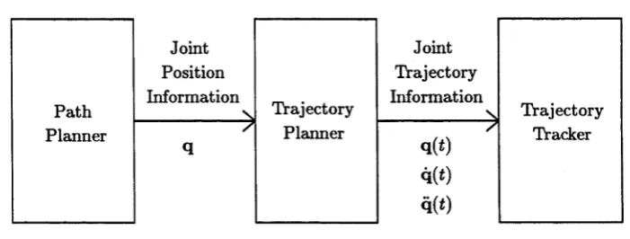
A variety of algorithms have been developed for planning and controlling the motion of robots. When the motion is constrained to a path, it has been usual to sub-divide the control problem into three separate levels; namely path planning, trajectory planning

and trajectory tracking, Figure 1.1. The reason for dividing the problem in this way is th at the collective problem is very complicated to solve because robot dynamics are usually highly nonlinear and coupled, and the control problem is of high dimension with multiple inputs and outputs.

Joint Trajectory Information Joint

Position Information

Trajectory Planner Path

Planner

Trajectory Tracker

Figure 1.1: The 3 Stages of Robot Motion Control

Path planning is concerned with the geometry of the desired task. The path planner would take into account kinematic constraints on the task, for example to ensure that obstacles are avoided, but might also consider dynamic constraints, for example to avoid configurations at which excessively high forces might be generated. The output of the path planner will be the joint position information, q, which may be represented either as a discrete set of points or via one or more continously parameterised functions. Many different path planning schemes have been proposed. However, this area is not the focus of our research and we would refer the reader interested in such schemes to, for example, [49] and references therein.

operates in discrete time.

There have been two main approaches to minimum-time trajectory planning, re­ flecting the two main approaches to optimal control generally. The first is based on the Pontryagin Maximum Principle [52] (such methods are sometimes referred to as

shooting methods in the path timing literature) and the second involves dynamic pro­ gramming. A more detailed discussion of these approaches is given in the descriptions of the problems th at we consider which follows in § 1.2. A comprehensive survey sum­ marising many of the results in the trajectory planning area can be found in [59].

In principle, the path and/or trajectory planning might be performed on-line. How­ ever, for anything more than the simplest of tasks, the computational complexity in­ volved presently requires th at this planning be done off-line.

The trajectory tracker is a part of the robot system. It consists of two parts; the trajectory generator and the tracking controller. The trajectory generator provides to the tracking controller the reference data calculated by the trajectory planner. The purpose of the tracking controller is to make the robot’s position and velocity match the reference position and velocity. Many different tracking controllers have been proposed, see for example [1] and references therein, although most often in practice a simple linear (PID) controller is used. Whilst the nonlinearities of the manipulator dynamics are not taken into account, such trackers can generally keep the manipulator reasonably close to the desired trajectory.

We note th at in contrast to earlier approaches for point-to-point motion control, some more recent work has combined the path and trajectory planning problems of this divided approach in order to obtain time-optimal trajectories for point-to-point motion control [25, 26, 32, 39, 56, 57]. These schemes have developed efficient search techniques in order to overcome the complexities involved in this unified approach.

• The application of dynamic programming to the problem of planning time-optimal trajectories for a robot manipulator whose motion is constrained to a path.

• The time-optimal control of robot manipulators along specified paths and to a specified tolerance in the presence of plant uncertainty.

• To investigate whether singular configurations would be good sites with respect to reducing the cycle times of pick and place operations.

These problems are now discussed in more detail.

1.2

T h e P rob lem s

P r o b le m 1: T ra jecto ry P la n n in g u sin g D y n a m ic P r o g r a m m in g

To use dynamic programming to plan the time-optimal motions of robot manipulators

constrained to specified paths.

Several approaches to the minimum-time trajectory planning problem noted th at the path constraint allows a reduction in the dimension of the state of the problem. The reduction is from typically 12, the joint positions and their derivatives, to 2, the path displacement and velocity [8, 51, 58, 60, 66]. This made calculation of a theoretically time-optimal trajectory feasible. Prior to this, assumptions and simplifications had to be made in order to solve the problem for “near” time-optimal solutions, [36, 42, 43, 71].

w ith singular points [54, 58].

N oting th e dim ension redu ctio n, o th er a u th o rs recognised th e p o ten tia l for using th e dynam ic program m ing m etho d to solve th e m inim um -tim e tra je c to ry planning problem [51, 61, 64]. T he real advantage in using dynam ic program m ing is n o t th a t it gives b e tte r solutions, b u t ra th e r th a t it readily allows solutions for c rite ria o th er th a n pure m in im um -tim e. W hile P o n try ag in ’s M axim um Principle can also h and le such c riteria, solution of th e resulting m ulti-dim ension 2-point b o u n d ary value problem is often less th a n triv ial, see for exam ple [55] where Shiller considers a “tim e-energy” perform ance c riteria. T h e approaches in [51, 61, 64] solve th e reduced-dim ension problem using B ellm an ’s recursion equation [7]. T his equ ation is discrete in th e s ta te s an d in tim e, a n d involves th e in teg ratio n of th e system dynam ics over a fixed tim e interval.

In our approach, we also consider th e application of dynam ic p rogram m ing to th e pro blem of th e planning of th e tim e-optim al m otion of ro b o t m an ip u la to rs along spec­ ified p a th s. However, we approach th e problem from a different asp ect th a n o ther dynam ic program m ing approaches to this problem . We consider th e num erical solution of th e continuous optim al-control problem , specified by th e H am ilton-Jacobi-B ellm an p a rtia l differential equation [41] using finite difference M arkov chain ty p e app rox im a­ tion s. O ur desire is to evaluate th e applicability of th e resu lting solutions to a real m a n ip u la to r and to analyse issues relating to th e convergence of th e approach.

P r o b le m 2: R o b u st T im e -O p tim a l P a t h T racking C o n tro l

To provide a systematic way of ensuring the accurate and time-optim al tracking of the specified path by a robot manipulator.

dynamics and that they take no account of the dynamics of the tracking controller which is used to reject the tracking errors.

Some more recent literature has attem pted to deal with these issues. The first approach involves quantifying the model parameter uncertainties and then making al­ lowances for them when planning the trajectory. Shin and McKay [62] devised an al­ gorithm for planning trajectories th at are robust to given payload uncertainties. They convert bounds on the payload uncertainty to bounds on the torque uncertainty and then plan time-optimal trajectories robust to the payload uncertainty by holding this amount of torque in reserve. Huang and Chen [34] also devise a scheme for dealing with payload uncertainty. This scheme has two parts. Off-line they calculate and tab ­ ulate the switching times for the problem based on several payload masses. On-line, and based on the system response, the payload is then estimated and the appropriate switching times chosen. Given its adaptability, the scheme in [34] has the ability to be less conservative than that in [62].

Another approach which can cope with small parameter uncertainty was proposed by Tam [68]. This is based upon a perturbation scheme which is applied in feedback and which amends the switching times to allow authority to control.

More recently, there has been a push towards considering robust control techniques, including 'H00 approaches, for the robust control of manipulators, [4, 19, 44, 53, 70] for example. However, very little of this work has focussed on the time-optimal control problem, which is more difficult to solve because the actuators are operating at their limits. The only contribution to date has been a theoretical approach by Lyashevskiy and Chen [50] who use Bellman-Lyapunov theory to find a closed-form solution for the optimal control in a point-to-point minimum-time control problem. It is interesting th a t their approach uses a non-minimum-time performance index.

time-scale (slow down or speed up) th e nom inal p a th trajecto ry . T h e nom inal p a th tra je c to ry is calculated using one of th e shooting or dynam ic program m ing m eth o d s described above. T h e approach consists of two p a rts. T h e desired on-line p a th acceleration is calcu lated as a function of th e nom inal p a th velocity an d acceleration, an d of th e on-line p a th positio n an d velocity. B ounds are th e n calculated on th e on-line p a th acceleration. T hese are based on th e on-line p a th position an d velocity, an d on m easured d a ta . N ext, th e on-line tra je c to ry inform ation is u p d a te d by in teg ratin g th e p a th acceleration, s a tu ra te d by th e on-line bou n d s if necessary. T h e on-line bound s on th e acceleration are designed so t h a t th e com m anded torques will not be clipped, so th a t th e end effector rem ains on th e desired p a th . However, because th e b o u nds are calcu lated from m easured d a ta , th ere can be no guaran tee th a t any valid b o un ds will exist, in which case th e com m anded torques will be clipped and a loss of track ing will occur. F u rth e r, th e desired p a th acceleration m ight be such t h a t no a c tu a to r is fully utilised. To overcome th is, th ey introduce th e idea of time-scaling of th e nom inal tra jec to ry . T h is idea provides a tim e shifting of th e nom inal tra je c to ry so th a t it is less or m ore d em and ing as required. Together, these ideas seem to provide good resu lts, a lth o u g h no co nsideration is m ade of th e accuracy of tracking and th e m eth o d requires th e tu n in g of filter p a ra m e te rs in an ap p aren tly ad hoc fashion.

D ahl an d N ielsen’s approach was later m odified by A rai et al. [2, 3] to resolve th e track ing error into com ponents tan g en tial a n d orthogonal to th e direction of m otion, a n d to place a higher p rio rity on reducing th e orthogonal com ponent. F u rth e r, th ey im ­ plem ented an observer to reduce th e am ount of co m p u tatio n of th e n onlinear dynam ics requ ired by th e m eth o d .

P r o b le m 3: Feist P ick a n d P la c e at K in e m a tic S in g u la r itie s

To investigate whether singular configurations would be good sites with respect to re­ ducing the cycle times of pick and place operations.

T h is piece of work is also concerned w ith fast ro b o t m otion, b u t considers a point- to -p o in t m otion control problem .

We hypothesise th a t singular configurations m ight be good sites a t which to perform pick and place operations, because th ey offer th e p o ten tial for reducing cycle tim es versus using neighbouring regular configuration sites. T h is is based on th e observation t h a t th e end effector can be b rou g h t to rest a t a singular configuration w ith o u t stopp ing th e m echanism , allowing th e ro b o t to keep some of its kinetic energy while perform ing th e pick or place task.

O u r aim is to investigate th is hypothesis.

We believe th a t th is idea is original and so we have no lite ra tu re w ith which to com pare our ideas.

1 .3

S u m m a r y o f C o n t r ib u tio n s

T ra jec to r y P la n n in g u sin g D y n a m ic P ro g r a m m in g

In th is work we considered applying dynam ic program m ing to solve th e problem of th e optim al p a th tim ing of ro b o t m an ipulators. O ur approach differed to previous dynam ic program m ing approaches to this problem in t h a t we solved num erically th e continuous optim al-control problem specified by th e Hamilton-Jacobi-Bellman p a rtia l differential equation of dynam ic program m ing using finite difference M arkov chain ty pe appro xim atio ns. O ur desire was to evaluate th e applicability of th e resu lting solutions to a real m an ip u la to r and to analyse issues relating to th e convergence of th is approach.

• We have applied solutions of th e dynam ic program m ing alg o rith m to a real SC A RA m an ip u lato r w ith good results

• We have shown th a t th e ra te of convergence of th e num erical schem e is consistent w ith th a t pred icted by theory.

• We have found th a t th e m inim um -tim e en d-point (ta rg e t) c o n stra in t im poses severe lim itatio n regarding th e ra te of convergence and co m p u tatio n al speed of th e dynam ic program m ing algorithm (in p a rticu la r, com m only used acceleration m eth o d s do n ot work).

• If a pure m inim um -tim e c riteria is required, th e P ontryagin M axim um P rinciple based shooting m eth od is superior an d is th e m eth o d of choice. However, th e dynam ic program m ing algorithm can easily handle m ore general o p tim isatio n c riteria , in which case th e advantages of th e P M P ap proach dim inish.

R o b u s t T im e -O p tim a l P a t h T racking C o n tro l

In th is work our goal was to provide a system atic way of controlling in d u stria l ro b o ts to achieve accu rate and tim e-optim al tracking of specified p a th s. T h e m ajo r issue th a t we ad dressed was to take previously developed th eory and to develop ways of m aking it p rac tic a l, to apply to real in d u strial robots. In p a rtic u la r, our focus has been to add ress th e issue of how a user specified trackin g tolerance can be achieved in spite of u nm odelled dynam ics.

To th is end, we have developed th re e m ajo r results:

• B ased on representing m odelling errors as distu rb an ces in jo in t accelerations, we have developed a th eo ry for relatin g these distu rb an ces to th e perform ance of a ro b o t u n d e r com p uted-to rq u e control. E x perim ental results confirm ed t h a t th e th eo ry works well in practice.

the disturbance using a trajectory close to the time-optimal trajectory being sought. The theory is then used to predict the torques th at need to be held on reserve during trajectory planning and the controller gains required to reject the disturbances to a specified tolerance. Experiments have shown th at if trajectories are planned and the controllers tuned in this way, then the robot performs near time-optimal tracking of the path, accurate to the specified tracking tolerance. • We have extended this method to a less conservative closed-loop architecture

which generates the trajectory on-line. We have proposed a feedback law for set­ ting the reference path acceleration such th at path tracking is nearly time-optimal, robustly controllable, and accurate to a prescribed tolerance. Experimental re­ sults have demonstrated th at the tracking times are reduced compared to the first approach, while the tracking accuracy and robustness remain approximately the same.

F ast P ick a n d P la c e at K in em a tic S in g u la r itie s

In this work we investigated whether singular configurations might be good sites, with respect to reducing cycle times, for pick and place operations.

• We have shown th at cycle times of pick and place operations can be reduced by placing the pick and place sites at kinematic singularities, compared to nearby regular configurations.

R e m a r k s o n t h e A p p lic a tio n o f

D y n a m ic P r o g r a m m in g to t h e

O p tim a l P a th T im in g o f R o b o t

M a n ip u la to r s

A b s t r a c t

In this chapter, we investigate the use of the dynamic programming approach in the. solution of the optimal path timing problem in robotics. This problem is computationally feasible because the path constraint reduces the dimension of the state in the problem to

2. The Hamilton-Jacobi-Bellman equation of dynamic programming, a nonlinear first

order partial differential equation, is presented and is solved approximately using finite difference methods. Numerical solution of this results in the optimal policy which can then be used to define the optimal path timing by numerical integration. Issues relating to the convergence of the numerical schemes are discussed, and the results are applied to an experimental SCAR A manipulator.

2 .1

I n tr o d u c t io n

Optimisation methods are commonly used in engineering design. In the context of

systems theory, two main approaches to optimal control have emerged: (i) Pontryagin

Maximum Principle (PMP) [52], (ii) Dynamic Programming (DP) [7]. The PMP is a set of necessary conditions th at an optimal control (if one exists) must satisfy, and is used to identify candidate open loop optimal controls. Dynamic programming involves the use of a value function and provides a means for determining optimal state feedback controls (verification theorem).

In many problems of interest in nonlinear control a state feedback controller is desired, and often such problems lend themselves to potential solution via dynamic programming, such as minimax (including Woo) control and stochastic optimal con­ trol. The usual difficulty with dynamic programming is the well known “curse of dimensionality” [7], and this limits the utility of DP in practice. Even if the optimal solution cannot be found (due to prohibitive computational costs), knowledge of the theoretically optimal solution can serve as a useful guide in designing implementable suboptimal controllers. However, there are some applications where the DP method is feasible. Such applications are of interest because they afford an opportunity to study practical issues relating to the DP method. Such issues include approximate (i.e. numerical) computation of the optimal state feedback controls, properties of the algorithms such as rate of convergence and memory requirements, and also real-time implementation issues. The purpose of this work is to study some of these issues in the context of optimal path timing for robot manipulators.

The optimal path timing problem has been studied extensively in the past. Typi­ cally, shooting techniques based on the PMP are employed, for example Bobrow et al.

[8] and Shin and McKay [60]. These methods assume knowledge of the bang-bang na­ ture of the optimal controls. Thus the DP and PM P methods can be directly compared in this application. Other papers using DP for this application include Pfieffer and Jo­ hanni [51] and Shin and McKay [61], although they solve the method in a different manner to th at presented below.

system ) w ith one control in p u t, s ta te d ep en d en t co n strain ts on th is in p u t a n d s ta te co n stra in ts, and reform ulate th e optim al control problem . In §2.4 we use dynam ic p rogram m ing m ethods to solve th e optim al control problem , an d presen t a num erical ap p ro x im atio n to th e solution based on th e num erical solution of th e H am ilto n-Jacob i- B ellm an (H JB ) p artial differential equation. T his num erical solution em ploys discreti­ satio n of th e s ta te space an d so provides discrete approxim ations to th e continuous solution. Solution of th e H JB equation provides th e value function (th e m inim um -tim e function in th e pure m inim um -tim e case), th e associated optim al feedback control pol­ icy (a feedback function of th e p a th position and velocity), and in form ation concerning th e con trollability of th e system . In §2.5 we present two exam ples based on a SCA RA m a n ip u la to r th a t we have in our laboratory. T he first is a pure m inim um -tim e exam ple, a n d th e second an exam ple using a m inim um -tim e plus s ta te an d control energy cri­ te ria which serves to d em o n strate th e versatility of th e dynam ic p ro g ram m in g m eth o d w hen dealing w ith problem s which have non bang-bang solutions. In b o th exam ples, we im plem ent th e resulting optim al solutions on th e SCARA m an ip u la to r to assess th e applicability of th e m eth od . In §2.6 we discuss th e co m p u tatio n al issues involved in th e calculation an d im p lem en tatio n of th e solutions, an d in §2.7 we consider th e effects of adding a discontinuous friction m odel into th e system dynam ics.

2.2

T h e T im e-O p tim a l P a th Tracking P ro b lem

C onsider a generalised n degree of freedom , rigid-body n o n -re d u n d a n t ro b o t. T he dynam ic equations m ay be w ritte n as

M ( q ) q + n ( q , q ) = T (2.1)

w here q E IRn are th e jo in t variables, T E IRn are th e jo in t a c tu a to r forces or torques whose co n strain ts, r ( q , q ) < r < r ( q , q ) , m ay be position a n d /o r velocity d e p e n d en t,

M (q ) E IRnxn is th e in e rtia m atrix , and n ( q ,q ) E IRn is th e vector con tain in g th e friction, coriolis, centrifugal force an d gravity term s.

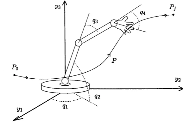
Figure 2.1: T he P a th To Be Traversed

jo in t variables th ro u g h th e kinem atic m apping y = r(q), and th e tim e-optim al problem is to find th e jo in t torques r ( t ) , 0 < t < t f, so th a t th e end-effector traverses a task space p a th P as fast as possible.

A ssum e th a t P is given as a regular, p aram etric curve, y = p ( s ), p E C 2, p aram e- terised by th e scalar s, so < s < Sf. T h en , q a n d s are rela te d by th e forw ard kinem atic eq u ation

r(q) = p (s) (2.2)

which we assum e can be solved th ro u g h inverse kinem atics for q = f (s ) .

A ssum ing an explicit and differentiable expression for f(s ) can be d eterm in ed , th e n th e sy stem dynam ics (2.1) can be re-expressed in term s of s ra th e r th a n q as

a ( s ) s -I- b ( s , s) = r (2.3)

w ith t(s,s) < T < r ( s , s), [8, 51, 58, 60]. T his form describes how th e control in p u ts

of equation (2.2), Slotine and Yang [66].)

The optimal control problem is now defined as:

Find the control T( t ) , T ( s ( t ) , s(t)) < T(t) < T( s( t ) , s( t ) ) , which minimises the perfor­

mance measure

J (s(0 ),s(0 )) = f f L( s( t ) , s( t ) , s{t ) ) d t , (2.4)

Jo

L (s,s, s) > 0 and L (s ,s ,s ) E C 2, subject to the dynamics (2.3) and to the boundary

conditions (s(0),s(0)) = (so>so) and {s(tf), s(tf)) = (s / , s / ) .

N o te: In the pure minimum-time case, L (s(i), s(£), r (t)) = 1, which yields J(s(0 ), s(0)) =

t f in (2.4).

2.3

R eform u lation o f th e P rob lem

In this section, we reformulate the problem into an equivalent second order state space

form with a single control input, state dependent constraints on the input, and state constraints, [8, 51, 60, 64, 66].

Let x\ = s and X2 = s . Then x\ = X2 and X2 = s , and equations (2.3) may be

rewritten in the equivalent nonlinear state space form:

or

1 0

0 ai( xi ) 0 o2(*i)

*2 -& i(x)

~b2(x)

+

0 0 0 - 0

1 0 0 - 0

0 1 0 - 0

n

T2

0 an(xi) _ -6 „ (x ) _ 0 0 0 - 1 Tn

(2.5)

E (x )x = A (x ) + B r . (2.6)

R em ark: Equation (2.6) differs from the usual nonlinear state space representation

due to presence of the E (x) matrix premultiplying x. This representation is known as

a nonlinear descriptor system form.

into a system equivalent form such that upper 2 x 2 sub-matrix of E (x) is diagonal and the rest is zero, but are prevented from using any one of the latter n rows as the

pivotal row because a^ xi) may equal zero for some x\. To circumvent this problem,

we define the path acceleration, s, to be a function of a new and independent control

ro,

* = ±2 = t o, (2.7)

augment equations (2.5) with (2.7), and row reduce the latter n equations of the aug­

mented system using the augmenting equation as the pivotal equation which allows the system (2.3) to be represented as follows:

1. Second Order System:

Xl ' 0 1 ‘ Xl

+ ’ 0 '

X 2 -1 O o

__

2. State and Control Constraints:

6i(x) a i(x i) Tl

• + T0 • = •

_ &n(x) _ _ an(*i) _ _{. Tn .} 3. Control Constraints:

(2.8)

r*(x) < T i < Tj(x), i = 1 to n.

Controls ri,...,rn can be eliminated from the problem by considering that equations

(2.8) can be satisfied for x if and only if

2i(x ) < bi(x) + ai(xi)ro < ri(x), i = 1 to n. (2.9) %

In (2.9), there are two possibilities, depending on whether a»(xi) = 0 or aj(xi) ^ 0. Let I (x i) = { i G {1,2, ...,n } : a;(xi) ^ 0 }.

If ai(x i) = 0, inequalities (2.9) can be written as state constraints t*(x) < 6i(x) <

t7(x). For a given x i, the set of all X2 simultaneously satisfying all such inequalities, denoted A z (xi), is

A z {xi) = P| {x2: 2i(x) < bi(x) < r7(x)} ,

and the region all x simultaneously satisfying all such inequalities, denoted

Az

A z

—

(^J-Az^l) •

Xi

Note that the inequalities defining

Az

Az

then the motion of the end-effector will not be constrained to the path and there will

exist no tq which will avoid this.

On the other hand, if a{(xi) ^ 0, the remaining inequalities of (2.9) can be rear­

ranged to give

i,(x) + tB £ L < To < _{S To S --- ;— r +}. . h ( x ) + ^ E L . T i ( x ) (2.10) a«(*l) ' M * l ) | U a«(*i) \a i ( x l ) \

In order that the end-effector tracks the path, there must exist at least one to satis­

fying all inequalities (2.10) simultaneously. Thus, the inequalities (2.10) act as state

constraints. For a given x i, the set of x2 simultaneously satisfying inequalities (2.10),

denoted

AnZ(x\),

b*(x)

Anz(x l) £ 2 • max

i e l ( x 1)

■ £ ( * ) } •

a,(xx) + M * ! ) ! / - < “ <*,)

j bj(x

\ a Ax

f bt(x) Ti(x)

\ Oj(®]':l) ' |a*(*i)|J

The region of all x simultaneously satisfying inequalities (2.10), denoted AnZ, is

A i z — A n Z{.X\) .

xi

In turn, for x € AnZ, to will be constrained to lie in an interval whose limits are a function of the state and determined by

max

* € / ( xi ) a » ( * i ) M * i ) U < r „ < min i e l ( x i ) { a i ( x 1) + | o i ( £ i ) | J

Define

A.

AnZ

A-z

Then we see that (2.9) can be solved for x if and only if x E

A.

A

admissible region.

Write

Wo(x) max

t € / ( x i )

bj{x) Tj(x) 1

at (Xl ) + l a i M I J ’i€/(xni)

Then we see th at Uq(x) = 0 if x & A and Z^o(x) ^ 0 if x G A. We will call ^o(x) the interval of admissible control values when in the state x.

The original optimal control problem is now equivalent to:

Find the control To(t) which minimises the performance measure

J ( x ( 0 ) ) = [ f L(x(t), T0(t)) dt , (2.11)

Jo

subject to the dynamics

*1 ' 0 1 ' X l

4 _ ’ 0 '

X2 _i o o *2 1 1

to the state and control constraints

x(i) 6 A, r 0(t) EZY0(x(t)), 0 < * < * , ,

where A and Wo(x) are defined above, and to the boundary conditions Xo = x(0) and

x / = x(t/).

Thus, we have reduced the problem of the simultaneous solution of n second order differential equations, to th at of the solution of one second order differential equation which is subject to state and control constraints.

2.4

S o lu tion o f th e E quivalent T im e-O p tim a l C ontrol

P rob lem

smooth, the optimal control policy can be determined from the HJB equation, via the verification theorem [30].

We define the value function, T (x), by

T(x) = inf

I

f

ro€Wo(x) L J o )

where x is the solution of (2.12) and ZJo(x) is the interval of admissible controls defined above. Notice th at T(x) G [0,+oo] and T(x) = +oo if x g A since £Yo(x) = 0- Also, T(x) < +oo if x is controllable to x /, otherwise T(x) = -foo. Let C denote the set of points controllable to xy. Then C C A .

The Hamilton-Jacobi-Bellman equation for the optimal-control problem is

0 = min (V T (x) • b(x,To) + L(x,ro)} , x G C

T o f z U o (x)

< T(xy) = 0

0 < T(x) < 1 if x ^ x f

T(x) = + 0 0 if x G dC

where b(x,ro) represents the system dynamics (2.12). The boundary conditions for this PDE are 5(xy) = 0 at the target state xy and S(x) = + 0 0 for x on the boundary

of the controllable subspace, dC.

Because T(x) = + 0 0 is difficult to deal with numerically, we consider the dis­

counted value function (see Bardi and Falcone [5] and Evans and James [29] for the case L (x (t),r0(t)) = 1).

S(x) = inf { [ e~Xh dsA L(x(t),ro(t),t) dt : x(0) = x x(ty) = x y l ,

tögWo(x) I Jo J

whence

S(x) = 1 - e ~ A:r(x), (2.13)

The HJB equation for the discounted optimal-control problem is 0 = min {V5(x) • b(x, ro) + AL(x, ro)(l — S(x))} , x G C

t0 €£4)(x)

< 5 ( x / ) = 0 (2.14)

0 < S(x) < 1 if x ^ x / S(x) = 1 if x E dC

The boundary conditions for this PDE are S (x /) = 0 at the target state X/ and

S ( x) = 1 for x on the boundary of the controllable subspace, dC. Note th at since the transformation (2.13) is monotonic, the minimising control To is the same for both the un-discounted and discounted problems.

If the HJB equation (2.14) has a smooth solution S(-), then the verification theorem of optimal control [30] implies th at if Tq(x) achieves the infimum in (2.14), then Tq (x) is an optimal feedback control, if sufficiently regular. However, in general, (2.14) does not have a smooth solution. In fact, typically S(-) is only Holder continuous with exponent 0 < a < 1 [5, 29] (such functions are not everywhere differentiable), and so does not satisfy (2.14) in a classical sense, but only in a weak sense, viz. the viscosity sense [31]. Because we cannot solve (2.14) explicitly, we must resort to a numerical approximation

S h(‘) of S(-). From this, an approximate optimal policy, Tq^x), will be obtained. Let V h be a rectangular grid of size h > 0 covering the admissible region A, or the

part of A of interest, Figure 2.2. Now, approximate V S(x) by a first order approxima­ tion over a grid of size h, so that

V S ( x ) • b(x, tq) ~

s ^ ±^ - s ^ ) bt(xTo)

bf = — b{ if b{ < 0, 5(x + hei) is taken when b{ > 0 and 5 (x — he*) when b{ < 0. Note th a t the difference quotient respects the system dynamics. This leads to algorithms with good stability properties, Kushner and Dupuis [41].

If we now define

v ( x ) = max | ^ | 6t ( x ,r 0) |} , A*h(x) = (2.16)

r0ez^(x) J v(x)

noting th at in our formulation v(x) is simply

v(x) = max {|x2| + |r0|} = |®2| + max {|r0(x)|, |tö(x)|} ,

T0eWo(x)

then using a modification of an algorithm presented by Kushner and Dupuis [41] (Chap­ ter 4, pp 76-77), the HJB equation (2.14) may be re-written in the form

S fc(x) = min <

r 0€Wo(x) 1

x G int V h

1 + AL(x,r0)A t/l(x)

f

\ z £ / S h (x)

S h( x , ) = 0

0 < 5^(x) < 1 if x 7^ x /

S h(x) = 1 if ^o(x) = 0 (x £ .4), or x G d V h

(2.17) where J\fh(x) = { x ,x ± hei} is the simplex consisting of x and its nearest neighbours in the discretised state space, V h,

P h{z\x,Tq)

6f ( x , r 0) v(x)

|fei(x,r0)| + |62( x ,r 0)| v(x)

if z = x ± hei

if z = x

an d we note th a t XIzgA/^x) P h(z|x, ro) = 1. T he num bers P h( z|x, ro) can be in te rp re te d as tra n sitio n probabilities for a controlled M arkov chain. K ushner an d D upuis show t h a t M arkov chain approxim ation m etho ds produce num erical schem es which have nice convergence prop erties, und er broad conditions.

L et S ^ x ) , x E V h, be th e solution of (2.17). T h en TqH {x.) E Uo(x) m inim ising th e righ t h an d side of th e P D E in (2.17) is th e desired ap p ro x im ation to Tq(x).

T h ere are two classical m eth od s of solving th e b o u n d ary value problem (2.17), nam ely th e value space or Jacobi m eth o d , which can be in te rp re te d as a fixed p o in t ite ratio n m eth o d , a n d th e policy space m eth o d which is analogous to a grad ien t procedure in th e space of controls, [41]. T h ere are also m any variations thereof, m ostly aim ed a t speeding up th e ra te of convergence. More discussion of co m p u tatio n al issues will be given in §2.6 after p resen tatio n of th e following exam ples.

2 .5

E x a m p le s

We now apply th e th eory developed in §2.2, §2.3 and §2.4 to exam ples based on an ex p erim en tal m an ip u la to r th a t we have in our laboratory. T h e m an ip u la to r is a 4 degree-of-freedom SCARA arm an d is described in A ppendix A. For sim plicity, we re s tric t th e m otion to be plan ar, driven by only th e first a n d second jo in t m otors.

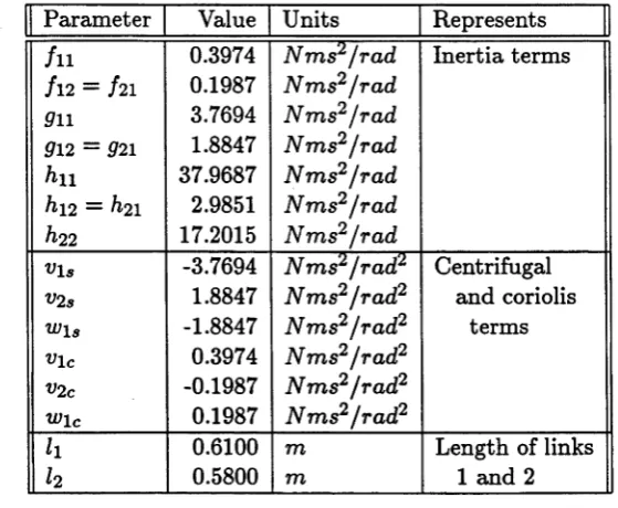
T h e p lan a r dynam ics of th e SCARA are m odelled as

M ( q ) q + v ( q , q ) = T (2.18)

w here M (q ) and v ( q ,q ) represent th e m ass m atrix and coriolis-centrifugal vector re­ spectively, a n d are defined in equations (A .2) and (A.3) of A ppendix A.

Param eter Value Units Represents h i 0.3974 N m s 2/r a d Inertia term s fl2 = /2 1 0.1987 N m s 2/ r a d

911 3.7694 N m s 2/ rad

912 = 921 1.8847 N m s 2/ rad

h\\ 37.9687 N m s 2/ r a d h \ 2 — h2\ 2.9851 N m s 2/ r a d h22 17.2015 N m s 2/r a d

V l s -3.7694 N m s 2/ r a d 2 Centrifugal

V 2 s 1.8847 N m s 2 / r a d 2 and coriolis

V J \ s -1.8847 N m s 2/ r a d 2 term s

V i c 0.3974 N m s 2/ r a d 2

v2c -0.1987 N m s 2/ r a d 2

V J \ c 0.1987 N m s 2/ r a d 2

h 0.6100 m Length of links h 0.5800 m 1 and 2

Table 2.1: SC ARA M anipulator Param eter D ata

The torque limits for this robot are given by

r ( q ) = max {-3 0 9 .4 2 ,-1 1 4 6 .0 - 984.987q> ^ r ( q ) = min {+309.42,+1146.0 - 984.987q}

J

(2.19)

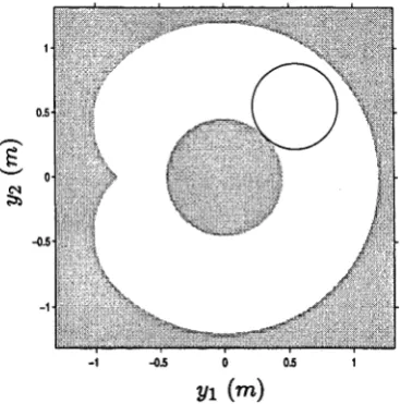
We choose the following joint space p ath param eterisation which traces a circle in the real physical space, Figure 2.3:

g i

92

arctan 2 ( ( W . M ) )

arccos (_V »i(*)+i/2 (*)-*?_2M2 i (s ) , (2.20) where

y i ( s ) = 0.55 — \/0.125cos(s) , V2(s) = 0.55 + \/0.125 sin(s) ,

a = l2 sm{q2) , ß = h + h cos (q2) ,

••

Figure 2.3: The Cartesian Space Path

Having specified the dynamics of the manipulator, (2.18), the torque limits, (2.19), and the joint path parameterisation, (2.20), we can now calculate the admissible region

A and admissible control space Z^o(x). Choosing h = 0.0125, these are displayed in Figures 2.4 and 2.5 respectively.

Figure 2.4: Admissible Region - A

50 v,

Figure 2.5: Adm issible Controls - Uq{x)

versus th e equivalent solution calculated using a P M P based shooting m eth o d . T he second criterion is a m inim um -tim e plus q u a d ra tic s ta te an d control cost which serves to d e m o n stra te th e versatility of th e dynam ic program m ing approach w hen calculating solutions which are n o t bang-bang in n a tu re .

2 .5 .1 P u r e M in im u m -T im e E x a m p le

In th e p u re m inim um -tim e case, we set L ( x (t) , ro(t)) = 1 which provides th e m inim um ­ tim e function T (x ) = fgf l d t = t f , as required. T h e num erical solution of th e cor­ responding H JB equation (2.17) th e n yields th e discretised discounted m inim um -tim e fu nction S h(’x ), from which th e m inim um -tim e can be recovered via

t f = “ X 1 0 ^ 1 '

Solu tion o f th e Exam ple

function S h(x) and the optimal control policy Tq^ x) shown in Figures 2.6 and 2.7. Note from Figure 2.6 that in this example, there are no points in the interior of A

where Sh(x) = 1. Thus, the controllable subspace C coincides with the admissible region A. (Other examples exist where Sh(x) is close to 1 in the interior of A. Such regions represent those states which are uncontrollable to the target state X f . )

-e CO

Figure 2.6: Value Function - Sh(x)

X

V 5

Using the initial state x(0) = 0, the discounted minimum-time function provides

S h(x) ~ 0.976 which predicts the minimum-time to complete the task as t f « 3.746s. We now integrate equations (2.12), choosing an initial state of x(0) = 0 and applying the optimal feedback control policy Tg^x) at each integration step by feeding back the state information. This yields the time-optimal path trajectories x*(<), displayed in the phase plane in Figure 2.8. The control To(t) achieving these trajectories, and the corresponding controls Tj(t) and r ^ t ) are shown in Figure 2.9. Note th at the time taken to reach the desired final state Xf is t f 3.727s which is marginally less than th at predicted by the discounted minimum-time function.

Figure 2.8: Optimal Path Trajectory - x^{x\)

The time taken for the system to reach the desired final state compares well with the minimum-time solution t f « 3.683s calculated using the PM P based shooting method of Bobrow et al [8]. The estimate is in error by only approximately 1%, which shows th at the numerical methods work well.

c

t (s)

Figure 2.9: Optimal Path Control -T*(t)=r*(x*(t))

A p p l i c a t i o n o f t h e R e s u l t

To im plem ent th is solution on our experim ental SCARA m an ip u la to r, we use a com puted- to rq u e controller, which is a m odel based-controller an d seems an a p p ro p riate choice given t h a t th e reference tra je c to ry which will drive th e ro b o t is calcu lated b ased on th e m odel.

T h e controller gains are chosen as k p = (100,100)T an d k v = (20,20) , an d cor­ resp o n d to critical dam ping and n a tu ra l frequencies of 10 r a d / s (sim ilar figures are com m only used in th e litera tu re ).

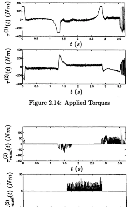
T h e tim e-o ptim al jo in t tra jec to rie s, Figure 2.10, are applied as reference to th e ex p erim en tal system and th e results logged. F igure 2.11 displays th e desired C artesian space p a th of th e end-effector, shown as th e solid line, a n d th e a c tu a l p a th tra c e d by th e end-effector, shown as th e dashed line. T h e tracking a p p ears to be qu ite good. However, if we exam ine a plo t of th e jo in t angle errors, Figure 2.12, we see t h a t th e erro r is ~ 0 (0 .0 5 rad) which th ro u g h th e forw ard kinem atics eq uates to approxim ately 5cm in th e end-effector position.

F igure 2.13 displays th e levels of com m anded torques th a t are clipped w hen th e a c tu a to rs s a tu ra te . C om paring th is to Figure 2.12, it is a p p a re n t t h a t th e jo in t angle errors, an d hence th e end-effector tracking error grow as th e a c tu a to rs sa tu ra te . T his is intu itiv ely obvious since th is is w hen th e ability to control to reject th e errors is lost.

In F igure 2.14, we see th a t th e torques dem and ed of th e a c tu a to rs contain some high frequency noise. E arly in th e tra je c to ry th e noise is not overly large, b u t late r on th ere are rap id oscillations in th e signal. A priori, our concern was th a t th is would m anifest itself as high frequency oscillations during th e experim ent. In fact, such oscillations were n o t visible d uring th e experim ent.

y i (m)

Figure 2.11: Cartesian Space Path - Predicted and Actual

Figure 2.12: End-Effector Tracking Error

t (s)

Figure 2.14: Applied Torques

Figure 2.15: Difference in Model Based Control for Numerical and Online Data

2 .5 .2 M in im u m -T im e P lu s Q u a d ra tic C o st E x a m p le

The second criterion that we consider is a minimum-time plus quadratic state and

control cost of the form

L(x(t),To(t)) = 1 + 0.25x2 + 0.02tq •

This example serves to demonstrate the versatility of the dynamic programming ap­

proach when calculating solutions which are not bang-bang in nature.

likewise, and also smooth out to, and hence the joint torques, at transitions (remember th at To = s and so we are limiting the acceleration).

Note th at this in this example, S h(x) is not the discounted minimum-time function. Thus, we cannot determine the time taken to traverse the path directly from S h(x).

Solu tion o f the Exam ple

Solution of the derived HJB equation (2.17), again choosing A = 1 for simplicity and using the same target state Xf = (6.3,0)T, yields the value function S h(x) and optimal control policy Tq^ x) shown in Figures 2.16 and 2.17 respectively . Notice in the optimal control policy the smoothing effect of the penalty on the control.

j;

Figure 2.16: Value Function - S h(x)

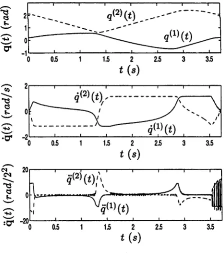
The optimal path trajectory, x*(t), is shown in the phase plane Figure 2.18. The control Tg (t) achieving this, and the corresponding controls Tj (t) and (t) are shown in Figure 2.19. The optimal joint trajectories q(t), q (t) and q (t) are shown in Figure 2.20.

causing much smoother transitions in the control signals (c./. Figure 2.9). Note finally the resulting increase in the time to complete the task compared to the pure minimum­ time case, from 3.723s to 4.300s.

Figure 2.17: Optimal Control Policy - r ^ f x )

-Figure 2.19: Optimal Path Control - r*(t)=T*(x*(t))

A p p lic a tio n o f th e R esu lt

We now implement the reference trajectory on our experimental SCARA manipulator, using the same computed-torque controller and gain settings as before.

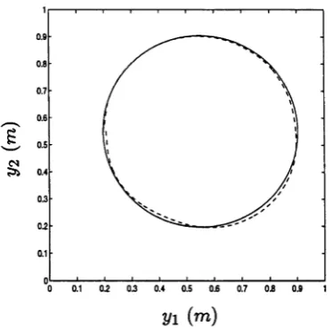
Figure 2.21 displays the desired Cartesian space path of the end-effector, shown as the solid line, and the actual path traced by the end-effector, shown as the dashed line. Clearly, the tracking is better than for the pure minimum-time example. Indeed, if we examine a plot of the joint angle errors, Figure 2.22, we see th at the error is now only ~ 0(0.03 rad), which through the forward kinematics equates to only approximately 3cm in the end-effector position.

Figure 2.23 displays the levels of commanded torques th at are clipped when the actuators saturate. It is again evident, by comparison to Figure 2.22, that the errors are correlated to the clipping of the commanded torques. However, we note th at the levels of clipping are less in this case than for the pure minimum-time example, c.f.

Figure 2.13, and so although there is no more ability to control the errors (this ability is lost as soon as the actuator saturates), the difference driving the errors is less.

Note in Figure 2.24, th at the level of noise present in the torques demanded of the actuators is much less than in the pure minimum-time example.

These results will be discussed in more detail in §2.6.

yi (m )

t (s)

Figure 2.22: End-Effector Tracking Error

T 200 !$; I«»

r \

N " -100 ^ • 8* ~ T3 -200

0.5 1 1.5 2 2.5 3 3.5 4

t (s)

T 20° l o o

—**— '“V

s ' -100 C S •«* 2 2* * 0 -200

0 0.5 1 1.5 2 2.5 3 3.5 4

t (s)

Figure 2.23: Torque Clipping

t (s)

2 .6

C o m p u ta t io n a l I s s u e s

A m ajo r issue w ith th e dynam ic program m ing m eth o d is co m p u tatio n al cost, viz. th e m em ory requirem ents and th e tim e required for com putations. T his depends critically on th e s ta te dim ension n: th e co m p u tatio n al cost grows exponentially w ith n (th e curse of dim ensionality). Since in th is problem th e dim ension is low (i.e. 2), co m p u ta tio n is feasible in practice, as we have d em o n strated . However, as w ith any num erical ap p ro x im atio n schem e, th ere is a tra d e off betw een co m p u tatio n al effort and accuracy.

As m entioned in § 2.4 above, th e discounted m inim um -tim e function S(-) is generally n o t everyw here differentiable, ra th e r only Holder continuous w ith exponent a, 0 < a < 1. T his lack of differentiability has im p o rta n t p ractical consequences. W ith o u t c o n stra in ts, th eory suggests a = ^, w ith ra te of convergence a n d th e error in th e ap p ro x im atio n e(h) ~ 0 (/i2), as th e step size h \, 0. O ur resu lts are consistent w ith th is predictio n , Figures 2.25 th ro u g h 2.28. T h is is a ra th e r slow ra te of convergence, m eaning th a t for th e error e(h) to be sm all, th e step size h m u st be very sm all w ith a consequent increase in th e m em ory requirem ents and co m p u tatio n al tim e. Indeed, th e n u m b er of iteratio n s to converge ap p ears to double as h is halved, while th e tim e to converge ap p ears to increase by a factor of 8, Figures 2.25 an d 2.26. T his d ram atic increase in tim e is of course due to th e to th e num ber of po ints in th e dom ain of calcu lation , an d hence also m em ory requirem ents, increasing by a factor of 4 as h is halved. T his slow ra te of convergence is due to th e ta rg e t-p o in t co n strain t.

A fu rth e r problem is th a t one m u st exercise care in d eterm in ing w hen th e num erical schem e has converged. O ur m easure of convergence 7 (-) com pares th e change in th e value fun ctio n relative to th e value function a t each ite ra tio n , viz

convergence is slow until it increases rapidly at 7 (k) ps 10- 8 , Figure 2.29. Unfortunately, the 7(A:) which signifies convergence is different for different examples, and would not

be known prior to solving the equation.

Considering all of these issues, it is important to solve the problem only as accurately

as required. If significant modelling errors, disturbances, etc., are anticipated then

errors of 5 — 10% might be seen as an acceptable engineering trade-off, and so h need

not be taken so small in practice. Also, we note that these computations are done off-line.

However, if high accuracy is important, there are schemes available to speed up the

rate of convergence. Details of many such schemes are given in [41]. In our work, we

tried a common acceleration scheme discussed by Capuzzo-Dolcetta and Falcone [27],

and Kushner and Dupuis [41]. In our theory, we specify two boundary conditions for solution of the PDE; on the boundaries of the admissible region d A and/or domain of

approximation &D, and at the target state X/. Unfortunately, the acceleration method failed due to the presence of the internal boundary condition at the target state xy, which is related to the Holder continuity of the (discounted) minimum-time function.

Without such a condition, substantial acceleration is possible, as advertised. (Note also that if the external boundary condition is removed, whilst the solution ultimately

converges to that calculated with the external boundary condition applied, there is a

substantial degradation in performance - it is not possible to remove the target state

boundary condition.)

We also tried multi-grid methods, where a solution calculated over a grid of size h is

interpolated into a new grid with hnew < h, and this then used as the initial guess for a

finer, and hence more accurate approximation. In fact, these methods proved fruitful.

Figure 2.30 displays the time savings when using multi-grid method which interpolates

a solution from a grid of size h to one of size The asterisks denote the time taken

for the solution to converge, in cpu mins, without using the multi-grid method, and the