Evolving boolean functions with conjunctions and disjunctions via genetic programming

This is a repository copy of

Evolving boolean functions with conjunctions and disjunctions

via genetic programming

.

White Rose Research Online URL for this paper:

http://eprints.whiterose.ac.uk/144390/

Version: Accepted Version

Proceedings Paper:

Doerr, B., Lissovoi, A. and Oliveto, P.S. (2019) Evolving boolean functions with

conjunctions and disjunctions via genetic programming. In: GECCO '19 : Proceedings of

the Genetic and Evolutionary Computation Conference. The Genetic and Evolutionary

Computation Conference - GECCO 2019, 13-17 Jul 2019, Prague, Czech Republic. ACM

Digital Library . ISBN 9781450361118

https://doi.org/10.1145/3321707.3321851

© 2019 The Authors. This is an author-produced version of a paper subsequently

published in GECCO 2019 Proceedings. Uploaded in accordance with the publisher's

self-archiving policy.

[email protected]

https://eprints.whiterose.ac.uk/

Reuse

Items deposited in White Rose Research Online are protected by copyright, with all rights reserved unless

indicated otherwise. They may be downloaded and/or printed for private study, or other acts as permitted by

national copyright laws. The publisher or other rights holders may allow further reproduction and re-use of

the full text version. This is indicated by the licence information on the White Rose Research Online record

for the item.

Takedown

If you consider content in White Rose Research Online to be in breach of UK law, please notify us by

Evolving Boolean Functions with Conjunctions and

Disjunctions via Genetic Programming

Benjamin Doerr

´Ecole Polytechnique, CNRS Laboratoire d’Informatique (LIX)

Palaiseau, France

Andrei Lissovoi

Deparment of Computer Science

University of Sheffield Sheffield, United Kingdom

Pietro S. Oliveto

Deparment of Computer Science

University of Sheffield Sheffield, United Kingdom

ABSTRACT

Recently it has been proved that simple GP systems can efficiently evolve the conjunction ofnvariables if they are equipped with the minimal required components. In this paper, we make a consid-erable step forward by analysing the behaviour and performance of the GP system for evolving a Boolean function with unknown components, i.e., the function may consist of both conjunctions and disjunctions. We rigorously prove that if the target function is the conjunction ofnvariables, then the RLS-GP using the complete truth table to evaluate program quality evolves the exact target function inO(ℓnlog2n)iterations in expectation, whereℓ ≥ n is a limit on the size of any accepted tree. When, as in realistic applications, only a polynomial sample of possible inputs is used to evaluate solution quality, we show how RLS-GP can evolve a conjunction with any polynomially small generalisation error with probability 1−O(log2(n)/n). To produce our results we introduce a super-multiplicative drift theorem that gives significantly stronger runtime bounds when the expected progress is only slightly super-linear in the distance from the optimum.

CCS CONCEPTS

•Theory of computation→Genetic programming;

KEYWORDS

Theory, Genetic programming, Running time analysis.

1

INTRODUCTION

Genetic Programming (GP) uses principles of Darwinian evolution to evolve computer programs with some desired functionality. The most popular and well-known GP approach, pioneered by Koza [11], represents programs using syntax trees. It uses genetic algo-rithm inspired variation operators to search through the space of programs that may be generated with the available components, and principles of natural selection to favour the ones which exhibit better behaviour on a wide variety of possible inputs. In this set-ting, program quality is evaluated by executing the constructed programs and comparing their output to the desired one.

Despite the many examples of successful applications of GP (see e.g. [1, 12, 15]), there is only a limited rigorous understanding of its behaviour and performance. While theoretical analyses exist, the available results have considered simplified GP systems, namely the RLS-GP and (1+1) GP algorithms, which evolve a program by applying a simple tree-based mutation operator called HVL-Prime to a single individual at a time for the evolution of non-executable tree structures [6, 7, 10], hence with no input/output behaviours.

Only recently, it has been proven that Boolean conjunctions ofnvariables can be evolved by RLS-GP [17] and (1+1) GP [14] algorithms in an expected polynomial number of iterations. The evolved conjunctions are exact when the complete truth table (i.e., the set of all 2npossible inputs) is used to evaluate solution quality, and generalise well when fitness is, more realistically, evaluated by sampling a polynomial number of inputs uniformly at random from the complete truth table in each iteration (i.e. employing Dynamic Subset Selection [8] to limit the total computational effort required to be polynomial with respect to the problem size).

While the mentioned results are promising, the considered GP systems were considerably different to those used in practice. In particular, they were required to evolve a simple arity-nBoolean conjunction from only its basic components (i.e. only the AND binary Boolean operator, and the inputs necessary for the problem). However in realistic applications, GP systems have access to a wider range of components than strictly necessary, because the required set of components is not necessarily known in advance. Ideally, the system should be equipped with a complete set of operators (i.e., a set from which any Boolean function may be constructed).

In this paper, we make a considerable step forward by analysing the behaviour and performance of RLS-GP for evolving an unknown Boolean function. More precisely, while the target function we consider is still ANDn, the conjunction ofnvariables, the GP system

has access to both the binary conjunction (i.e., AND) and disjunction operators (i.e., OR). Using ANDnas the target function simplifies

our understanding of the quality of candidate solutions that mix conjunction and disjunction operators.

This more complex problem setting induces us to introduce more sophisticated features into the RLS-GP system than those neces-sary to evolve conjunctions using the AND operator alone, thus making the GP system more similar to realistic applications. Since the presence of disjunctions in the current solution may reduce the effectiveness of the mutation operator at producing programs with better behaviour, we introduce a limit on the size of the syn-tax tree. This allows us to avoid issues due to bloat (a common problem for GP systems, where the size of the solution is allowed to increase without a corresponding increase in solution quality [11, 20]). While alternative bloat control measures, such as lexi-cographic parsimony pressure [16], would prevent RLS-GP from adding any unnecessary disjunctions entirely, a limit on the tree size is likely required to avoid pathological cases for more sophisticated insertion operators such as that of the (1+1) GP, which would be able to accept disjunctions if the mutation operator simultaneously improves the solution in some other fashion.

With the limit on the tree size in place, our theoretical analysis reveals that the HVL-Prime mutation operator used in previous

work [7, 14], which either inserts, substitutes or deletes one node of the tree, may get stuck on local optima. Hence, the expected runtime of RLS-GP with the traditional HVL-Prime operator has infinite expected runtime. To this end we introduce a mutation mechanism closer to the most commonly used subtree mutation [11, 20], specifically allowing deletion to remove entire subtrees in one operation, rather than limiting it to only a single leaf and its immediate parent.

We show that RLS-GP with the above modifications is able to cope efficiently with the extended function set. In particular we prove that using the complete truth table to evaluate program quality, and rejecting any tree with more thanℓ₌(1+c)n(where c>0 is a constant) leaf nodes, it evolves the exact target function inO(ℓnlog2n)iterations in expectation. While using the complete truth table to evaluate program quality requires exponential time, we consider this setting for two main reasons: first, this setting represents the best-case model of the GP system’s behaviour (i.e. a system unable to find the optimal solution when given access to a reliable fitness function is unlikely to be able to perform well with a noisy one); and second, the deterministic fitness values somewhat simplify the behaviour of the algorithm and hence our analysis.

Afterwards we consider more realistic training sets of polyno-mial size sampled in each iteration uniformly at random from the complete truth table. In practice some information about the func-tion class to be evolved may be used to decide which inputs to use in the training set. For instance, if the target function was known to be the conjunction ofnvariables, then a compact training set of linear size would suffice to evolve the exact solution efficiently [14]. How-ever, we assume that the target function is an unknown arbitrary function composed of conjunctions and disjunctions ofnvariables. Our aim is to estimate the quality of the solution produced by the RLS-GP in this setting.

We show that with probability 1−O(log2(n)/n)RLS-GP is able to construct and return a conjunction with a polynomially small generalisation error in a logarithmic number of iterations. Hence, if multiple runs of the GP are performed as in practice, a solution that generalises well is generated with probability converging quickly to 1 with the number of runs.

To achieve our results, we introduce a super-multiplicative drift theorem that makes use of a stronger drift than the linear one required by the traditional multiplicative drift theorem [5]. This new contribution to the portfolio of methodologies for the analysis of randomised search heuristics [13, 19] allows for the achievement of drastically smaller bounds on the expected runtime in the presence of a strong multiplicative drift.

We complement our theoretical results with an empirical inves-tigation that, on one hand, confirms our theoretical intuition that leaf-only deletion may get stuck on local optima if a limit on the tree size is imposed for bloat control reasons. On the other hand, while the experiments indicate that the algorithm would evolve the solution more quickly without a limit on the tree size, the size limit reduces the amount of expected undesired binary disjunction operators in the final solution.

Algorithm 1The RLS-GP algorithm with a tree size limitℓ.

1: Initialise an empty treeX 2: fort←1,2, . . .do

3: X′←HVL-Prime(X)

4: ifLeafCount(X′) ≤ℓandf(X′) ≤ f(X)then

5: X ←X′

2

PRELIMINARIES

In this work, we will analyse the performance of the simple RLS-GP algorithm on the ANDnproblem: evolving a conjunction of alln

input variables while usingF ={AND,OR}binary functions and L={x1, . . . ,xn}input variables. When program quality is

evalu-ated using the complete truth table, the fitness functionf(X)counts the number of truth-value assignments on which the candidate solu-tionXdiffers from the target function ˆh(x_{)=ANDn=x1∧. . .∧xn.}

From [14], we repeat the observation that a conjunction ofadistinct variables differs from ANDnon 2n−a−1 rows of the complete truth

table.

We will analyse the performance of the RLS-GP algorithm, which repeatedly chooses the best between its current solution and an offspring generated by applying the HVL-Prime mutation operator, which with equal probability inserts, deletes, or substitutes a leaf node in the current solution [7]. We observe that the presence of disjunctions in the current solution may lead to bloat issues: each OR increases the minimum number of leaf nodes required to represent the exact conjunction (up to a factor of at most 2, depending on its position within the tree), can be difficult for HVL-Prime to remove (as its deletion sub-operation only removes a single leaf node and its immediate ancestor), and may additionally slow the progress toward the optimum (as insertions under an OR have a diminished effect on the overall solution semantics). To counteract this, we add a simple bloat control mechanism to RLS-GP, making it reject trees which contain more thanℓleaf nodes, as described in Algorithm 1.

With the tree size limit in place, applying the original HVL-Prime mutation operator [7] may cause RLS-GP with the limitℓto get stuck on a local optimum.

Theorem 2.1. The expected optimisation time of RLS-GP with leaf-only deletion and substitution sub-operations of HVL-Prime, and any

ℓ >0on ANDnwithF={AND,OR}is infinite.

Proof. It is possible for RLS-GP to construct trees which cannot be further improved by local mutations. One example of this is a tree constructed by initially creating a disjunction ofℓ/2x1leaf

nodes, and then transforming eachx1leaf into anx1∧x2subtree.

No leaf node in the final tree can be deleted or substituted without decreasing fitness, and no insertion will be accepted due to the tree size limit, rendering RLS-GP unable to reach the optimum. As this tree can be constructed with non-zero probability, the expected time to construct the optimal solution is infinite by the law of total

expectation.

To avoid this issue, we modify the deletion operation of HVL-Prime to allow deletion of subtrees as described in Algorithm 2.

We use the termsampled errorto refer to the fitness value of a particular solution in a particular iteration, andgeneralisation error

Algorithm 2HVL-Prime with subtree deletion on treeX.

1: Chooseop ∈ {INS,DEL,SUB},l ∈ L, f ∈ F uniformly at random

2: ifXis an empty treethen

3: Setlto be the root ofX.

4: else ifop=INSthen

5: Choose a nodex ∈Xuniformly at random

6: Replacex withf, setting the children off to bex andl, order chosen u.a.r.

7: else ifop=DELthen ⊲modified (subtree) deletion

8: Choose a nodex ∈Xuniformly at random

9: Replacex’s parent inXwithx’s sibling inX 10: else ifop=SUBthen

11: Choose a leaf nodex∈X uniformly at random

12: Replacexwithl.

13: returnthe modified treeX

to refer to the probability that a particular solution is wrong on an input chosen uniformly at random from the set of all 2npossible inputs. When program quality is evaluated using the complete truth table, the sampled error of a solution is always exactly 2n times its generalisation error. When the complete truth table is used, the goal of the GP system is to construct a solution that is semantically equivalent to the target function i.e., achieve a sampled (and generalisation) error of 0.

As it is computationally infeasible to evaluate all 2n possible inputs for larger values ofn, we also analyse the behaviour of RLS-GP when evaluating solution quality based ons∈poly(n)inputs chosen uniformly at random from the set of all possible inputs. A fresh set ofsinputs is chosen in each iteration, and f(X), or

thesampled error, then refers to the number of inputs, among the

chosens, on whichX differs from the target function. The sampled error is thus a random variable, and its expectation is exactlystimes the generalisation error of the solution. We bound the probability of the sampled error deviating from its expectation in Lemma 2.2 below. When a polynomial training set is used to evaluate program quality, the goal of the GP system is to construct a solution with a low generalisation error. OnANDn, and most other non-trivial

problems, we do not expect the GP systems to reach a generalisation error of 0 whilesremains polynomial with respect to the problem size, unless the problem’s fitness landscape is well understood and a problem-specific training set is used. We assume that this is not the case, and that the aim is to find a solution that has a polynomially small generalisation error.

Lemma 2.2. Lets∈poly(n)be the number of inputs sampled by

the GP system,Fbe the generalisation error of a solution, andX be a

random variable denoting the sampled error of that solution. Then,

for anycthat is at least a positive constant,

|Fs−X| ≤max{clgn,Fs}

with probability at least1−n−Ω(c).

Proof. X is a sum ofsBernoulli variables, each with a prob-abilityF of assuming the value 1 (and 0 otherwise), and hence E[X]₌Fs. As bothXandFsare non-negative,Fs−X ≤Fs, and

we focus solely on the case whereX significantly exceeds its ex-pectation, the probability of which can be bounded by applying a Chernoff bound.

Suppose thatE[X] ≥ (c/2)lgn; then, Pr[X ≥ (1+1)E[X]] ≤

e−E[X]/3 ≤n−Ω(c); and hence|Fs−X|<Fs, with probability at least 1−n−Ω(c). Otherwise, we upper boundE[X] ≤µ+_=(c/2)lgn,

and apply a Chernoff bound usingµ+_{[3, Theorem 66], obtaining}

Pr[X ≥ (1+1)µ+_{] ≤e}−µ+_/3

=n−Ω(c); and hence|Fs−X| ≤X ≤

clgnwith probability at least 1−n−Ω(c).

Finally, we use the following notation throughout the paper: N _{:= {0},1,2, . . .}, lg(n) and ln(e)denoting the base 2 and the natural logarithms ofn, while lognis used in asymptotic bounds.

3

COMPLETE TRUTH TABLE

In this section, we will present a runtime analysis of the RLS-GP algorithm with subtree deletion (i.e., Algorithm 1) on theANDn

problem, using the complete truth table to evaluate solution quality, i.e. executing each constructed program on all 2npossible inputs.

Theorem 3.1. The expected runtime of RLS-GP withℓ ≥non

ANDnisE[T]=Ω(nlogn).

Proof. No tree which does not contain allndistinct variables can be equivalent to theANDn function. By a standard coupon

collector argument,Ω(nlogn)insertion or substitution operations are required to insert allndistinct variables into the tree.

The following drift theorem deals with the situation that the expected progress when in distancedfrom the target is of order

Ω(dlogd). This assumption is slightly stronger than the linear, that is,Ω(d), progress assumed in the multiplicative drift theorem. De-spite this apparently small difference, the resulting bounds for the expected time to reach the target differ drastically. For an initial dis-tance ofd0, they are, roughly speaking,O(logd0)for the

multiplica-tive drift situation andO(log logd0)for our super-multiplicative

drift.

Theorem 3.2 (super-multiplicative drift theorem). Letγ >

1andδ >0. LetX0,X1, . . . be random variables taking values in

Ω₌{0} ∪ [1,∞). Assume that for allt∈N_{and allx} ∈Ω\ {0}such

thatPr[Xt=x]>0we have

E[Xt−Xt+1|Xt =x] ≥ (log_γ(x)+1)δx. (1)

Then the first hitting timeT =min{t∈N|Xt =0}of zero satisfies

E[T |X0] ≤ 3 δ +

2(2+log2logγmax{γ,X0})lnγ

δ .

Proof. For allk∈N_{≥1, letTk :=min}{t ∈N|Xt <γ2

k−1

}. We first show that

E[Tk−Tk+1] ≤

1+2klnγ

(2k−1_+1)δ

holds for allk≥1. To this aim, we regard the processYtdefined

for allt ∈N_{byYt =Xt ift} ≤Tk−1 andYt =0 otherwise. By definition,T_kY :=min{t ∈N|Yt <γ2

k−1

}satisfiesT_kY =Tk. The

process(Yt)satisfies the multiplicative drift condition

E[Yt−Yt+1|Yt] ≥ (2k−1+1)δYt.

This follows from treating separately the trivial caseYt =0 and the more interesting caseYt ≥γ2

k−1

and exploitingYt+1≤Xt+1,

Yt =Xt, and (1) in the latter case.

LetTY :=min{t∈N_{|Yt=0}. SinceT}Y _=TY

k =Tkand since

Yt ≤γ2

k

for allt ≥Tk+1, the multiplicative drift theorem [5] yields

E[Tk−Tk+1]=E[TY −T_kY₊₁] ≤ 1+lnγ 2k (2k−1_+1)δ =

1+2k

lnγ

(2k−1_+1)δ.

By a simple application of the multiplicative drift theorem, we also observe thatE[T−T1] ≤ 1+_δlnγ.

In the following, we condition on the initial valueX0. Assume

thatX0∈ [γ2

k−1

,γ2k)for somek∈N_{≥1. ThenTk}

+1=0 and thus T =Íki=1(Ti−Ti+1)+(T−T1). We compute

E[T]₌

k

Õ

i=1

E[Ti−Ti+1]+E[T−T1] ≤ k

Õ

i=1

1+2ilnγ

(2i−1_+1)δ +

1+lnγ δ

≤ 3

δ +

2(k+1)lnγ

δ ≤

3 δ +

2(2+log2logγX0)lnγ

δ .

ForX0<γ, we have in an analogous wayE[T] ≤ 1+ln_δ(X0) ≤1+_δlnγ.

This proves the claim.

The proof of the above theorem estimates the super-multiplicative drift by piece-wise multiplicative drifts. We preferred this proof method because of its simplicity and because it could, by using the multiplicative drift theorem with bounds [4], also lead to tail-bounds for super-multiplicative drift as well (we do not elaborate on this as we do not need tail bounds). An alternative approach which would improve the time bound by a constant factor (again a feature we are not interested in here) would be to use variable drift [9, 18].

We use the super-multiplicative drift theorem to prove our upper bound for the runtime of RLS-GP on theANDnfunction. We start

by bounding the time spent in iterations in which the tree is not full, that is, it has not reached the size limit of havingℓleaf nodes.

Lemma 3.3. Consider a run of RLS-GP on ANDn, using a tree size

limit ofℓ≥n. LetT be the number of iterations before the optimum

is found, andT0≤T be the number of these iterations in which the

parent individual is not a full tree. Then,E[T0]=O(ℓnlog2n).

Proof. To boundE[T0], we will apply Theorem 3.2 using

so-lution fitness as the potential function, and considering only the iterations in which the tree is not full. While the treeisfull, we instead rely on the elitism of the RLS-GP algorithm to not accept mutations which increase the potential function value (i.e., off-spring with a worse fitness value). Thus, theT0iterations in which

the tree is not full need not be contiguous.

In an iteration starting with a tree containing less thanℓleaf nodes, it is possible to insert a new leaf nodexi with anAN D

parent anchored at the root of the tree. We call such an operation a root-and. The probability that in one iteration a root-and with a fixed variablexiis performed, is at least 1₃·1₂·₂1ℓ·n1 = 121ℓn.

We compute the expected fitness gain caused by such modifi-cations. Because the fitness never worsens, it suffices to regard certain operations that improve the fitness. Recall further that the fitness is just the number of assignments to the variablesx1, . . . ,xn

such that the tree evaluates differently fromANDn(“contradicting

assignments”).

Letx1, . . . ,xnbe such an assignment. This implies that not allxi

are true, because any tree generated by RLS-GP evaluates correctly to true for the all-true assignment. Assume that exactlyk≥1 of the variablesx1, . . . ,xnare false, but that our tree solution evaluates to

true. Then there are exactlykvariables such that a root-and with one of them would make this assignment evaluate to false (and thus improve the fitness since this assignment is not contradicting anymore). The probability for such a mutation is at least₁₂k_ℓn.

For any 1 ≤i ≤ n, there are exactly n_i

assignments where exactlyi variables are set to false, and hence there are exactly

Ík−1

i=1 n i

possible assignments where less thankvariables are set to false. Therefore, if the fitness of the current solution is at least Mk=2Íki=−11

n i

, at least half of the assignments contributing to the fitness have at leastkvariables set to false. Only regarding the progress caused by these, we have, forx ≥Mk,

Ef(Xt) −f(Xt+1_{) |f(X}t₎

=x≥ 1

12ℓ

k

nx. (2) Since fornsufficiently large we haveMk ≤2nk−1for allk ∈

[1..n]. This implies that for allx∈ [1..2n]and allt ∈N_{, we have}

E

f(Xt) −f(Xt+1_{) | f(X}t₎

=x ≥ ₁₂1_ℓ

n(⌊logn(x/2)⌋+1)x

≥ 1

36ℓn(logn(x)+1)x, where the last estimate usesn≥2. Hence Theorem 3.2 withγ =n andδ=1/36ℓngives

E[T] ≤36ℓn(3+2(2+log2logn2n))lnn)=O(ℓnlog2n).

We can then show that the conditions required to apply Lemma 3.3 occur sufficiently often to not affect the asymptotic expected run-time.

Theorem 3.4. Consider a run of RLS-GP on ANDn, using a tree

size limit ofℓ₌(1+c)n. LetTbe the number of iterations before the

optimum is found. Ifc=Θ(1), thenE[T]=O(ℓnlog2n).

Proof. To prove the theorem, we combine the result of Lemma 3.3 with an argument showing that with high probability, the parent solution contains fewer thanℓleaf nodes in at least a constant fraction of anyt∈Ω(ℓnlog2n)iterations.

LetT′ =c∗ℓnlog2n, for some constantc∗ > 0, be an upper bound on the expected number of iterationsE[T0]in which the tree

is not full before the optimum solution is found per Lemma 3.3. By an application of Markov’s inequality, the probability that the optimum is found in at most 2T′such iterations is at least 1/2. We will show that ifℓ ₌(1+c)n, for any constantc >0, 2T′such iterations occur in(2+c′)T′iterations with high probability, where c′>0 is constant with respect ton. The theorem statement then follows from a simple waiting time argument: during each period of

(2+c′)T′iterations, the optimum is found with at least probability 1/2· (1−o(1))₌Ω(1), so the expected number of such periods before the optimum is found is at mostO(1), and thus the expected runtime is at mostO(T′)₌O(ℓnlog2n)iterations.

at most increase the number of leaf nodes in the tree by 1, there will with high probability be at leastc′′Niterations in which the tree is not full among any(1+c′′)Niterations. AsT′∈Ω(ℓnlog2n), 2T′ iterations in which the tree is not full will with high probability occur in(2+c′)T′iterations wherec′=2/c′′=Ω(1).

Consider a treeXwith exactlyℓleaf nodes. LetLA(X)be a set of

leaf nodes connected to the root ofX via only AND nodes, and call

essentialall the leaf nodes in this set that contain a variable which

only appears on nodes in this set exactly once. IfX is non-optimal, at mostn−1 leaf nodes inX are essential, and at leastℓ− (n−1)

leaf nodes are non-essential. All non-essential nodes are either directly deletable (in the case of redundant copies of variables in LA(X)), or indirectly deletable (by deleting a branch at any of their

OR ancestors).

Every non-essential leaf node can thus be deleted by performing an HVL-Prime deletion sub-operation on at least one node in the tree. For some non-essential leaf nodes, a larger subtree may need to be deleted to remove the leaf without adversely impacting fitness. The longer waiting time for such subtree deletions (requiring that the root of the subtree be chosen for deletion rather than one of the many leaf nodes in the subtree) is balanced by the increased number of leaf nodes deleted as part of the mutation. We note that the tree contains 2ℓ−1 nodes, and thus forℓ≥ (1+c)nand any c>0, an HVL-Prime mutation in expectation reduces the number of leaf nodes in the tree by at least

E[∆] ≥ 1

3

ℓ− (n−1)

2ℓ−1 ≥

ℓ−n 6ℓ ≥

c

6+6c ≥δ ∈

Ω(1),

whereδ >0 is a positive constant, asc∈Ω(1).

LetX1, . . . ,XN be the number of leaf nodes deleted in an

ac-cepted mutation during each iteration performed while the tree is full, andX =ÍNi=1Xi. Furthermore, define a sequenceZ0, . . . ,ZN,

whereZ0 := 0 andZi := Zi−1+Xi −δ; clearly,ZN −Z0 = ZN =X −δ N. We will show thatZN >−δ N/2 (and therefore

X >δ N/2∈Ω(N)) holds with high probability.

AsE[Zi |Z1, . . .Zi−1]=Zi−1+E[Xi |Z1, . . .Zi−1] −δ ≥Zi−1,

the sequenceZ0, . . . ,ZNis a sub-martingale, andci :=|Zi−Zi−1| ≤

ℓ. Hence, by applying the Azuma-Hoeffding inequality forN ∈ Ω(ℓnlog2n)andt=δ N/2,

Pr[ZN−Z0≤ −t] ≤exp

−t2 2ÍN

i=1c2i

!

≤exp

−δ2N

8ℓ2

≤n−Ω(logn)

asN/ℓ2₌Ω(nℓlog2n/ℓ2)₌Ω(log2n)forℓ₌(1+c)nwherecis a constant.

Thus, there exists a constantc′′>0 such that over the course ofN ∈Ω(nℓlog2n)iterations where the tree is full, deletions of at leastδ N/2=c′′N leaf nodes are accepted with high probability, and hence over the course of 2/c′′Niterations, at least 2Niterations occur while the tree is not full with high probability. SettingN = T′ = c∗nℓlog2niterations per Lemma 3.3 completes the proof: amongΘ(T′)iterations, at leastΩ(T′)will take place while the tree is not full, allowing the application of the Markov inequality and waiting time arguments to produce the bound on the expected

runtime.

4

POLYNOMIALLY SIZED TRAINING SETS

While Theorem 3.4 provides a polynomial bound on the number of iterations required to evolve the conjunction ofnvariables, calcu-lating solution quality by evaluating the output of the candidate solution and the target function on each one of the 2n possible inputs in each iteration requires exponential computational effort, and is thus only computationally feasible for relatively modest values ofn.

In this section, we consider the behaviour of the RLS-GP algo-rithm when using only a polynomial computational effort in each iteration. To this end, the solution quality is compared by evaluat-ing the output of the ancestor solution, the offsprevaluat-ing, and the target function on only a polynomial number of inputs (“the training set”), sampled uniformly at random from the set of all possible inputs in each iteration. This setting was previously considered in [14], where it was shown that the RLS-GP and the (1+1) GP algorithms usingF ={AN D}are able to construct a solution withO(logn)

distinct variables which fits a polynomially large training set in polynomial time.

For our main theoretical result below, we opt to have RLS-GP ter-minate and return a solution once the sampled error on the training set is below a logarithmic acceptance threshold. This effectively pre-vents RLS-GP from entering a region of the search space where the mechanism it uses to evaluate program quality is overly noisy. This slightly decreases the expected solution quality, but does preserve the overall guarantee on the quality of the produced solution.

Theorem 4.1. For any constantc>0, an instance of the RLS-GP

algorithm withF ={AN D,OR},L={x1, . . . ,xn},ℓ≥n, using a

training set ofs=nclg2nrows sampled uniformly at random from

the complete truth table in each iteration to evaluate solution quality, and terminating when the sampled error of the solution is at most

c′lgn, wherec′is an appropriately large constant, will with

proba-bility at least1−O(log2(n)/n)terminate withinO(logn)iterations,

producing a solution with a generalisation error of at mostn−c.

To prove this theorem, we will show that RLS-GP is able to create a tree that contains no more than one copy of each variable, no OR functions, and enough distinct variables to sample an error below the acceptance threshold withinO(logn)iterations with probability at least 1−O(log2(n)/n). Additionally, we will show that with high probability, the GP system will not terminate early (i.e., it will not return a solution with a generalisation error greater thann−c).

Lemma 4.2. If RLS-GP never accepts solutions containing OR nodes or multiple copies of any variable, and never accepts solutions with a

worse generalisation error than their ancestors, it will withinO(logn)

iterations reach a solution with a sampled error belowc′lgn, where

c′>0is an appropriate constant, with probability at least1−O(1/n).

Proof. To ensure that an error belowc′lgnis sampled, we con-sider the time required to construct a solution with an expected sampling error of at most(c′/4)lgn. Such a sampling error can be achieved by a generalisation error of at most((c′/4)lgn)/(nclg2n)₌ (c′/4)n−c/lgn≥n−(c+1)_{(for a sufficiently largen), i.e., a} conjunc-tion of(c+1)lgnvariables or more.

ANDnode, and using a Chernoff bound to show that a sufficient number of such insertions occur within a particular number of iterations (as the number of distinct variables in the current so-lution is never reduced by the lemma’s conditions). Specifically, suppose that the current solution containsi <n/2 distinct vari-ables and no OR nodes, and letXi be the event that a mutation

inserts a new variable and connects it to the tree using an AND node, and is accepted. We bound Pr[Xi] ≥ (1/3)(1/2)(n−i)/n≥δ,

i.e.,δ ≥1/12 fori<n/2. The probability that at least(c+1)lgn such mutations are accepted within(c′′/δ)(c+1)lgn=O(logn)

iterations is then, by applying a Chernoff bound [2, Lemma 1.18], at least 1−e−Ω(c′′logn)=1−n−Ω(c′′). Thus, whenc′′is a sufficiently large constant, this probability is at least 1−O(1/n).

We bound the probability that a solution with a low-enough expected sampled error does not meet the acceptance threshold by applying Lemma 2.2: once a solution with an expected sampled error of at most(c′/4)lgnis constructed, the probability that its sampled error exceeds the acceptance threshold is at mostn−Ω(c′), and thus, whenc′is picked appropriately, the solution is accepted immediately with probability at least 1−O(1/n).

By combining the failure probabilities using a union bound, we conclude that RLS-GP under the conditions of the lemma and with an appropriately-chosen constantc′, is able to construct a solution with an acceptable sampled error withinO(logn)iterations with probability at least 1−O(1/n).

We will now use this bound on the runtime of RLS-GP to show that it is likely to avoid all of the potential pitfalls preventing the application of Lemma 4.2.

Lemma 4.3. With probability at least1−O(log2(n)/n), during its

firstO(logn)iterations and while the expected sampled error of its

current solution remains above(c′/4)lgn, RLS-GP is able to avoid

accepting mutations which: (1) insert copies of a variable already present in the current solution, (2) insert OR nodes, or (3) increase the generalisation error of the current solution.

Proof. For claim (1), we note that within the firstO(logn) it-erations, the tree will contain at mostO(logn)distinct variables (as each iteration of RLS-GP is only able to insert one additional variable). Thus, the probability that a mutation operation adds a variable which is already present in the solution (using either the insertion or substitution sub-operation of HVL-Prime) is at most O(logn/n), and by a union bound, this does not occur during the firstO(logn)iterations with probability at least 1−O(log2(n)/n).

For claim (2), we note that there are two main ways an OR can be introduced into the solution by an insertion operation: either the OR is semantically neutral (which, if the ancestor contains only ANDs and unique variables requires replacing a leafxiwithxi∨xi),

or the sampling process used to evaluate solution fitness did not sample any inputs on which the offspring is wrong and the ancestor is correct. We will consider the two possibilities separately.

As semantically-neutral insertions of OR nodes require inserting a duplicate copy of a variable, claim (1) already provides the desired probability bound on these insertions not occurring withinO(logn)

iterations (and hence not being accepted). All other OR insertions will increase the generalisation error of the solution. The magnitude of this increase depends on the number of distinct variables in the

subtree displaced by the insertion, with insertions displacing only a single leaf node being the easiest to accept.

If a leaf of the ancestor solution is replaced with a disjunction with a new variable, we use the termwitnessto refer to inputs which set the displaced variable to 0 while setting the remaining variables in the offspring solution to 1. As the offspring solution also differs from the target function on all the inputs on which the ancestor solution does so, as long as the sampling procedure sam-ples at least one witness, RLS-GP will reject the mutated solution. Suppose the ancestor conjunction containsUdistinct variables; it is then incorrect on 2n−U −1 possible inputs, while there are at least 2n−(U+1)_{witnesses; i.e. the probability of randomly selecting}

a witness is at least half that of randomly selecting a row on which the ancestor is wrong. Thus, if the expected sampled error of the ancestor solution is at leastX, the expected number of witnesses in the sample is at leastX/2. By a Chernoff bound, the probability that fewer than(c′/16)lgnwitnesses are present in the sample is at moste−(c′/128)lgn =n−Ω(c′). By setting the constantc′ appro-priately, this probability can be made intoO(1/n), and by a union bound, the probability that no OR which increases the generalisa-tion error is accepted withinO(logn)iterations while the expected sampled error of the solution remains above(c′/4)lgnis at least 1−O(log(n)/n).

Finally, for claim (3), we note that decreasing the number of dis-tinct variables in the solution more than doubles its generalisation error. Applying a similar argument for rejecting detrimental ORs above (this time, the expected number of witnesses in the sample is at leastX), the probability that no mutations increasing the gen-eralisation error are accepted duringO(logn)iterations is at least 1−O(log(n)/n).

Combining the error probabilities of the three claims using a union bound yields the theorem statement.

Finally, we show that with high probability, RLS-GP does not terminate unacceptably early (i.e. by sampling an error below the acceptance threshold for a solution with a worse generalisation error than desired by Theorem 4.1).

Lemma 4.4. With high probability, no solution with a

generalisa-tion error greater thann−chas a sampled error of at mostc′lgnon

a set ofs≥nclg2nrows sampled random from the complete truth

table, within any polynomial number of iterations.

Proof. Recall that when samplingsrows uniformly at random from the complete truth table to evaluate solution fitness, RLS-GP terminates and returns the current solution when the solution appears wrong on at mostc′lgn of the sampled rows. As the generalisation error of a solution is also the probability that the solution is wrong on a uniformly-sampled row of the complete truth table, a solutionXwith a generalisation errorд(X)of at leastn−c, has an expected sampled errorE(f(X)) ≥lg2nons=nclg2nrows sampled uniformly at random. Applying a Chernoff bound, the probability that the sampled errorY is less than half of its expected value (which for large-enoughnis above thec′lgnthreshold), is super-polynomially small:

Pr[Y ≤1/2E[Y]] ≤e−E[Y]/8≤n−Ω(logn).

∨

∧

x3 x2 ∧

x2 x3

∧

∨

∧

∧

x2 x3

x5 ∧

x2 ∧

x3 x5

x1

∧

∨

∧

x3 ∧

x5 x7 ∧

x3 ∧

x7 x5 ∧

x2 ∧

[image:8.612.57.294.81.154.2]

x8 x4

Figure 1: Examples of locally optimal trees, which cannot be improved by substitution or have any single leaf deleted without affecting fitness, constructed by RLS-GP using leaf-only substitution and deletion operations.

Bya union bound, RLS-GP with high probability does not return a solution with a generalisation error of at leastn−c within any polynomial number of iterations when samplings =Ω(nclg2n)

rows of the complete truth table uniformly at random to evaluate solution quality in each iteration.

Our main result is proved by combining these lemmas.

Proof of Theorem 4.1. By Lemma 4.3, the conditions neces-sary to apply Lemma 4.2 occur with probability at least 1−O(log2(n)/n), and thus with probability at least 1−O(log2(n)/n) −O(1/n), a so-lution with a sampled error meeting the acceptance threshold will be found and returned withinO(logn)iterations. By Lemma 4.4, the generalisation error of any solution returned by RLS-GP within a polynomial number of iterations is with high probability better

than the desiredn−c.

We remark that performingλruns of RLS-GP, as is often done in practice, and terminating once any instance determines that its current solution meets the acceptance threshold, will guarantee that a solution with the desired generalisation error is produced usingO(λlogn)fitness evaluations with probability 1−n−Ω(λ).

5

EXPERIMENTS

We performed experiments to complement our theoretical results. For each choice of algorithm and problem parameters, we per-formed 500 independent runs of the GP system.

Theorem 2.1 showed that using the standard HVL-Prime oper-ator, which applies leaf-only deletion and substitution, can cause RLS-GP with the complete truth table to get stuck on a local op-timum when a tree size limit is imposed, thus leading to infinite expected runtime. However, the theorem does not provide bounds on the probability that this event occurs. Table 1 summarises the experimental behaviour of RLS-GP. The experiments confirm that when using small tree size limits, RLS-GP indeed gets stuck on local optima. Examples of the ones constructed during the runs are depicted in Fig. 1. However, the probability of getting stuck decreases asℓ, the limit on the size of the tree, increases. Con-cerning solution quality, with small tree size limits, the number of redundant variables in the final solution decreases at the expense of higher runtimes. Forℓ₌n,‘exact’solutions are returned when the algorithm does not get stuck. On the other hand, larger tree size limits (including no limit) lead to smaller expected runtimes at the expense of redundant variables in the final solutions.

ℓ₌n ℓ₌n+1

n B T S B T S

4 0.008 46.3 (28.0) 4.0 (0.0) 0.002 40.9 (21.8) 4.4 (0.5) 8 0.002 151.8 (91.9) 8.0 (0.0) 0.004 113.8 (51.5) 8.6 (0.5) 12 0.016 284.1 (148.2) 12.0 (0.0) 0.002 214.3 (99.5) 12.7 (0.5) 16 0.008 469.9 (258.0) 16.0 (0.0) 0.010 345.8 (161.0) 16.8 (0.4)

ℓ₌2n ℓ₌∞

n B T S B T S

4 0 42.5 (25.8) 5.1 (1.2) 0 38.9 (24.3) 5.4 (2.0) 8 0 98.8 (49.0) 11.0 (2.3) 0 95.3 (43.8) 11.2 (3.0) 12 0 170.7 (99.7) 17.1 (3.3) 0 160.1 (57.1) 17.9 (4.5) 16 0 232.5 (80.9) 23.8 (4.1) 0 235.3 (92.7) 24.6 (6.0) Table 1: Proportion of runs stuck in a local optimum (B), and average runtime (T) and solution size (S) of successful runs of the RLS-GP using leaf-only substitution and deletion with the complete truth table to evaluate solution quality for varyingnandℓ. Standard deviations appear in parentheses.

ℓ₌n ℓ₌n+1 ℓ=2n ℓ=∞

n T S T S T S T S

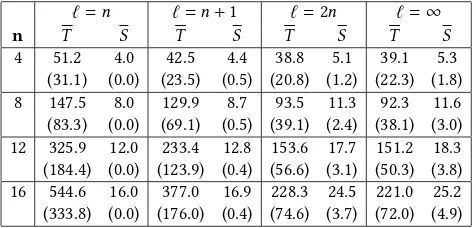
[image:8.612.318.561.82.230.2]

4 51.2 4.0 42.5 4.4 38.8 5.1 39.1 5.3 (31.1) (0.0) (23.5) (0.5) (20.8) (1.2) (22.3) (1.8) 8 147.5 8.0 129.9 8.7 93.5 11.3 92.3 11.6 (83.3) (0.0) (69.1) (0.5) (39.1) (2.4) (38.1) (3.0) 12 325.9 12.0 233.4 12.8 153.6 17.7 151.2 18.3 (184.4) (0.0) (123.9) (0.4) (56.6) (3.1) (50.3) (3.8) 16 544.6 16.0 377.0 16.9 228.3 24.5 221.0 25.2 (333.8) (0.0) (176.0) (0.4) (74.6) (3.7) (72.0) (4.9) Table 2: Average runtime (T) and solution size (S) of RLS-GP using the subtree deletion sub-operation, and the complete truth table to evaluate solution fitness, for varyingnandℓ. Standard deviations appear in parentheses.

We now turn our attention to the HVL-Prime modified to allow subtree deletion, as considered by Theorem 3.4. As predicted by the theory, RLS-GP never gets stuck in our experiments when using the complete truth table and a tree size limit. Table 2 shows the average number of iterations required to find the global optimum for various problem sizes and varying tree size limits. Once again the experiments show that smaller tree size limits lead to lower numbers of redundant variables at the expense of a higher runtime. Larger limits, including no limit at all, lead to faster runtimes at the expense of admitting more redundant variables. Noting that in practical applications a tree size limit is often necessary, we leave the proof that the algorithm evolves an exact conjunction without any limits on the tree size for future work.

[image:8.612.320.558.311.425.2]

101 102 103 104 105 106 0

20 40 60 80 100 120

Training Set Size (rows)

Runtime

(iterations)

A=0 A=8

A=16

A=32

101 102 103 104 105 106

0 5 10 15 20

Training Set Size (rows)

Solution

Size

(leaf

no

des)

A=0

A=8 A=16

[image:9.612.58.290.78.364.2]

A=32

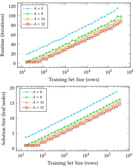
Figure 2: Average runtime and tree size produced by RLS-GP with subtree deletion, using an incomplete training set, stop-ping once sampled error is at mostA,n=50, ℓ₌∞, averaged over 500 independent simulations.

in Figure 2. The figure confirms our theoretical result that the algorithms generally run in logarithmic time and produce solutions that contain a logarithmic number of leaf nodes with respect to the training set size. Stopping at 0 error, though, leads to better solutions at the expense of higher runtimes. Figure 3 shows the average number of ORs in the final solution. While these are small in number, they grow as the stopping criteria, i.e. the threshold on acceptable sampled error, decreases.

6

CONCLUSION

In this paper, we analysed the behaviour of a variant of the RLS-GP algorithm, providing rigorous runtime bounds when using the complete truth table to evaluate solution quality, as well as when using a polynomial sample of possible inputs chosen uniformly at random. Equipped with a tree size limit and a mutation operator capable of deleting entire subtrees, RLS-GP is able to efficiently evolve a Boolean function –ANDn, the conjunction ofnvariables –

when given access to both the binary conjunction and disjunction operators.

When using the complete truth table to evaluate the quality of solutions, we show that in expectation, an optimal solution is found withinO(ℓnlog2n)iterations. Experimentally, we see that the GP system is able to find solutions quicker asℓ, the limit on the tree size, increases, suggesting that the theoretical bound is overly pessimistic

101 102 103 104 105 106

0 0.2 0.4 0.6 0.8 1

Training Set Size (rows)

ORs

accepte

d

during

run

A=0

A=8

A=16 A=32

101 102 103 104 105 106

0 0.1 0.2 0.3 0.4

Training Set Size (rows)

ORs

in

returne

d

solution

A=0 A=8

A=16 A=32

Figure 3: Number of OR nodes inserted and surviving to the solution returned by RLS-GP with subtree deletion, using an incomplete training set, stopping once sampled error is at mostA,n = 50, ℓ ₌ ∞, averaged over 500 independent simulations.

in its modelling of the process. Conversely, solutions with larger tree size limits tend to contain more redundant variables, suggesting a trade-off between optimisation time and solution complexity.

When sampling a polynomial number of inputs to evaluate pro-gram quality, the evolved solutions are not exactly equivalent to the target function, but generalise well: any polynomially small gener-alisation error can be achieved by sampling a polynomial number of inputs uniformly at random in each iteration. Our theoretical results predict that RLS-GP is usually able to avoid inserting ORs in this setting, which is reflected in our experimental results.

While these results represent a considerable step forward for the theoretical analysis of GP behaviour, much work remains to be done: apart from the open problem of removing the limit on the tree size, the analysis could be extended to cover yet larger function sets (e.g. by also including NOT, allowing the GP to express any Boolean function), introducing more variables than required by the target function, or considering a more complex target function where populations and crossover may be required.

Acknowledgements.Financial support by the Engineering and

Physical Sciences Research Council (EPSRC Grant No. EP/M004252/1) is gratefully acknowledged.

[image:9.612.322.553.81.365.2]

REFERENCES

[1] Alberto Bartoli, Simone Cumar, Andrea De Lorenzo, and Eric Medvet. 2014. Compressing Regular Expression Sets for Deep Packet Inspection. InProceedings of Parallel Problem Solving from Nature - PPSN XIII.394–403.

[2] Benjamin Doerr. 2011. Analyzing Randomized Search Heuristics: Tools from Probability Theory. InTheory of Randomized Search Heuristics, Anne Auger and Benjamin Doerr (Eds.). World Scientific, 1–20.

[3] Benjamin Doerr. 2018. Probabilistic Tools for the Analysis of Randomized Opti-mization Heuristics.CoRRabs/1801.06733 (2018). arXiv:1801.06733

[4] Benjamin Doerr and Leslie A. Goldberg. 2013. Adaptive drift analysis. Algorith-mica65 (2013), 224–250.

[5] Benjamin Doerr, Daniel Johannsen, and Carola Winzen. 2012. Multiplicative Drift Analysis.Algorithmica64, 4 (2012), 673–697.

[6] Benjamin Doerr, Timo K¨otzing, J. A. Gregor Lagodzinski, and Johannes Lengler. 2017. Bounding bloat in genetic programming. InProceedings of the Genetic and Evolutionary Computation Conference (GECCO 2017). 921–928.

[7] Greg Durrett, Frank Neumann, and Una-May O’Reilly. 2011. Computational complexity analysis of simple genetic programming on two problems model-ing isolated program semantics. InProceedings of the Foundations of Genetic Algorithms workshop (FOGA 2011). 69–80.

[8] Chris Gathercole and Peter Ross. 1994. Dynamic Training Subset Selection for Supervised Learning in Genetic Programming. InProceedings of Parallel Problem Solving from Nature - PPSN III.312–321.

[9] Daniel Johannsen. 2010.Random combinatorial structures and randomized search heuristics. Ph.D. Dissertation. Universit¨at des Saarlandes, Saarbr¨ucken. [10] Timo K¨otzing, Andrew M. Sutton, Frank Neumann, and Una-May O’Reilly. 2014.

The MAX problem revisited: The importance of mutation in genetic programming.

Theoretical Computer Science545 (2014), 94–107.

[11] John R. Koza. 1992.Genetic programming - on the programming of computers by means of natural selection. MIT Press.

[12] John R. Koza. 2010. Human-competitive results produced by genetic program-ming.Genetic Programming and Evolvable Machines11, 3-4 (2010), 251–284. [13] Per Kristian Lehre and Pietro S. Oliveto. 2017. Theoretical Analysis of Stochastic

Search Algorithms. InHandbook of Heuristics (to appear), Rafael Marti Mauricio G.C. Resende and Panos M. Pardalos (Eds.). Springer. arXiv:1709.00890 [14] Andrei Lissovoi and Pietro S. Oliveto. 2018. On the Time and Space Complexity of

Genetic Programming for Evolving Boolean Conjunctions. InProceedings of the Thirty-Second AAAI Conference on Artificial Intelligence. AAAI Press, 1363–1370. [15] Li Liu and Ling Shao. 2013. Learning Discriminative Representations from RGB-D

Video Data. InProceedings of the 23rd International Joint Conference on Artificial Intelligence (IJCAI 2013). 1493–1500.

[16] Sean Luke and Liviu Panait. 2002. Lexicographic Parsimony Pressure. In Pro-ceedings of the Genetic and Evolutionary Computation Conference (GECCO 2002). 829–836.

[17] Andrea Mambrini and Pietro S. Oliveto. 2016. On the Analysis of Simple Ge-netic Programming for Evolving Boolean Functions. InProceedings of Genetic Programming - 19th European Conference (EuroGP 2016). 99–114.

[18] Boris Mitavskiy, Jonathan E. Rowe, and Chris Cannings. 2009. Theoretical analysis of local search strategies to optimize network communication subject to preserving the total number of links.Int. J. Intelligent Computing and Cybernetics

2, 2 (2009), 243–284.

[19] Pietro S. Oliveto and Xin Yao. 2011. Runtime analysis of evolutionary algorithms for discrete optimization. InTheory of Randomized Search Heuristics: Founda-tions and Recent Developments, Anne Auger and Benjamin Doerr (Eds.). World Scientific, Chapter 2, 21–52.

[20] Riccardo Poli, William B. Langdon, and Nicholas Freitag McPhee. 2008.A Field Guide to Genetic Programming. http://lulu.com.