A simplified creep-reverse plasticity solution method for bodies subjected to cyclic loading

(1)

A simplified creep-reverse plasticity solution method

for bodies subjected to cyclic loading

Haofeng Chen and Alan R.S. Ponter

Department of Engineering, University of Leicester, Leicester, LE1 7RH, UK Email: [email protected], [email protected]

Tel: 0044-1162522549 Fax: 0044-116252252

Abstract: An extension of the upper bound shakedown theorem to load histories in excess of shakedown has been applied recently to the evaluation of a ratchet limit and the varying plastic strain magnitudes associated with a varying residual stress field. Solutions were obtained by the Linear Matching Method. In the present paper, this technique is extended to the evaluation of creep-reverse plasticity mechanism for bodies subjected to thermal cyclic loading including creep effects. The accumulated creep strain, the varying flow stress and the corresponding varying residual stress field during a creep dwell time are evaluated as well as the elastic follow-up factor. Three alternative computational strategies are discussed with differing but related assumptions. The problem of a plate with a central circular hole is discussed, subjected to cyclic thermal load. All three methods provide similar values for the elastic follow-up factor, indicating that the result is insensitive to the range of assumptions made. The simplest method, Method 1, is suggested as the basis of a general purpose method for use in life assessment.

Keywords: cyclic loading, creep, reverse plasticity, elastic follow-up

NOTATION

(2)

E

E, Young’s modulus and effective modulus for uni-axial and multi-axial conditions

ε

σ

,

stress and strain

dt

t

,

, τ times 2

1,t

t , Δt time instances and creep dwell time

p

ε

Δ , Δεc _{plastic strain range and accumulated creep strain}

c

p ρ

ρ Δ

Δ , varying residual stress associated with reverse plasticity mechanism and creep relaxation

rp ij ε

Δ total varying strain

Dc, N0 creep endurance limit and cycles to failure

ij

σˆ applied linear elastic stress field

ij

ρ , ρ_ij(t) constant and changing residual stress field

μ

, K Linear elastic shear modulus and modulus of compression pr

i

u

Δ displacement increment c

σ , Δεijc creep stress and creep strain

0

σ

, ε&₀, n creep materials data

c ij

ε& creep strain rate

θ θ

θ, 0,Δ temperatures

E, S, P, R elastic, shakedown, reverse plasticity and ratchetting region ε

σ, & von Mises effective stress and strain rate in

ij

σ initial stress field for creep computation

D, L diameter of the hole and length of the plate

0

t

σ maximum von Mises effective elastic thermal stress ν

σ_Y, yield stress and Poison’s ratio

(3)

1. Introduction

The processes of engineering design and life assessment of structures subjected to cyclic loading require the evaluation of load histories for which certain types of material failure occur (Ainsworth, 2003; Ainsworth and Budden, 1992). The prediction of these failure mechanisms of structures with variable repeated loading is significant and has attracted the attentions of many researchers (Chen and Ponter, 2001a, 2001b; Chen et al., 1999, 2003; Engelhardt, 1999; Ponter and Chen, 2001; Maier, 1977; Corradi and Zavelani, 1974; Hachemi and Weichert, 1998; Mackenzie et al., 1996; Seshadri and Mangalaramanan, 1998; Boyle et al., 1997) generally using programming methods.

(4)

amplitude and the proximity to a ratchet limit, based upon a new minimum theorem (Ponter and Chen, 2001).

In practice, components can operate at high temperature within the creep range both within shakedown and for load ranges in excess of shakedown. Typically, in power plant, a creep dwell periods exist where the temperature of some proportion of the structure lies within the creep range. For some components, e.g. heat exchangers, the mechanical loads can be relatively small but the thermal stresses can be significantly in excess of yield. In such circumstances creep strains occur, and this results in the relaxation of initially high stresses as creep strains replaces elastic strains. Lifetime integrity may then be limited not only by low cycle fatigue but the damaging effects of the creep strains produced during creep relaxation. The evaluation of the creep relaxation, the determination of the accumulated creep strain, the varying flow stress and the corresponding elastic follow-up factors during dwell period are very important components of life assessment methods. The work of this paper is part of a general study of the application of the Linear Matching Method to the various stages of Life Assessment methods, using R5 (Ainsworth, 2003; Ainsworth and Budden, 1992) as the beginning point. It is anticipated that such methods may then replace the rule-based methods currently used, providing more accurate and less conservative predictions.

The term “elastic follow-up” has been used to describe the effects of creep strains in local regions where the total strain increases through interaction with the overall elastic compliance of the structure (Ainsworth, 2003). The concept was introduced to allow the local accumulation of creep strain to be estimated without the need to performing full time-dependent structural analysis. The process may be described for a uniaxial state of stress by an equation of the form:

0 = +Z d

dε_c σ

(5)

where Z is the elastic follow-up factor, E is Young’s modulus, εc is the creep strain accumulated during the dwell, and

σ

is the applied stress. The factor Z characterises the stress-strain path followed during stress relaxation. For example, Z=1 corresponds to relaxation at a constant total strain and Z →∞ corresponds to creep at a constant stress. Although equation (1) is an approximation, in detailed calculations of relaxation, Z is found to be relatively constant in time.

For a restricted class of problems, where the stress relaxes proportionally throughout the structure, an analytic solution for Z may be computed. All of the known solutions are of this type (Hubel and Zeibig, 1996). In Appendix 1 we give a general derivation of this result and apply the result to three simple examples where creep occurs throughout the structure or, alternatively, in only part of the structure. These solutions demonstrate that the variation of Z values between otherwise similar structures can be significant. Accurate assessments of Z and creep accumulation may only be achieved through an accurate description of the initial stress and the variation of the creep rate throughout the structure during the dwell period.

(6)

2. Elastic Follow-up factor Z for Proportional Relaxation

For certain simple problems the stress relaxes according to the simple equation )

( )

(t _ij0f t

ij σ

σ = (2)

where 0 ij

σ is the stress at time t=0. In this case Z may be evaluated explicitly;

c

D U

Z _~

~ 2

&

= (3)

where U~ is the total elastic strain energy and D~&c is the total creep energy dissipation rate, both evaluated for 0

ij

σ . Each quantity is normalised with respect to the stress at the location where Z is

required, usually the position of maximum von Mises effective stress. The derivation of this result is given in Appendix 1. A valuable insight into the dependence of Z on the characteristics of the problem is also provided.

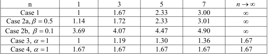
Using these formulations in Appendix 1, we can evaluate Z for simple beam structures. Table 1 lists the variation of Z for two simple beam structures with creep index n. The detailed analysis is given in Appendix 2. Generally Z increases with n but there are significant differences in behaviour. For a typical value of n=5, Z has values across the range 1.3≤Z≤4.47. From these results we observe that an accurate assessment of Z is only possible if the initial stress is modelled effectively and the variation of the creep rate throughout the structure is properly modelled. The methods described in the next section are designed to achieve these ends.

3. Definition of the problem

(7)

and the elastic behaviour is isotropic. A schematic of a typical load history is shown in Fig.1. The structure is subjected to high temperature into the creep range, beginning at time t₁ followed by a dwell period Δt and then a return to low temperatures at times t2. Hence creep relaxation occurs

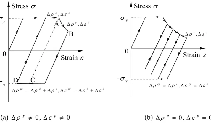
in the body during dwell period Δt and reverse plasticity appears in the body at times t₁and t₂. This paper discusses two kinds of creep-reverse plasticity mechanisms for the cyclic loads shown in Fig. 1. Fig. 2a shows, schematically, the case where the load range exceeds the reverse plasticity limit, and the plastic strain increment Δεijp as well as the associated residual stress range p

ij ρ

Δ occurs at both extremes of the load cycle. This is determined before the evaluation of

the accumulated creep strain Δεijc and the corresponding residual stress c ij ρ

Δ for creep relaxation.

The total varying strain Δεijrp is the summation of p ij ε

Δ andΔεijc. Fig. 2b shows the case where the

load variation is below the elastic shakedown limit, i.e. Δ =0,Δ p =0 ij p

ij ρ

ε , and the total varying

strain c

ij rp ij ε

ε =Δ

Δ in the steady state. In order to understand the difference between pure reverse

plasticity mechanism (Ponter and Chen, 2001; Chen and Ponter, 2001b) and creep-reverse plasticity mechanism proposed in this paper, Fig. 3 presents a schematic representation of the plastic and creep quantities in the above two mechanisms in biaxial stress space. For the pure reverse plasticity mechanism (Fig.3a), there are two plastic strain increments associated with two load extremes. For the creep-reverse plasticity mechanism (Fig.3b), the strain increment during loading cycle is split into two increments, i.e. the plastic strain increment and the creep strain increment. Note that the accumulated creep strain c

ij ε

Δ is shown as associated with a flow stress

(8)

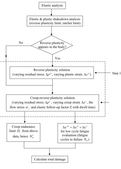
Fig. 4 gives a flow chart for the creep-reverse plasticity solution method. The first step in all three methods is to perform a reverse plasticity solution method (Ponter and Chen, 2001; Chen and Ponter, 2001b) and calculate the varying plastic strain Δε_ijp and the varying residual stress p

ij ρ

Δ . This step can be ignored (Fig. 2b) when the applied load domain is below the elastic

shakedown limit. The second step is to perform a creep-reverse plasticity solution method, where the initial elastic stress amplitude has been amended by the varying residual stress Δρijp associated with pure reverse plasticity mechanism. This results in an additional change in residual stress c

ij ρ

Δ during the creep dwell Δt and an accumulated magnitude of creep strain c ij ε

Δ . The

details of how this may be done will be presented in the next several sections. In the context of the life assessment method R5, once Δε_ijc and the corresponding residual stress Δρ_ijc are determined, the elastic follow-up factor Z, the creep endurance limit Dc, the number of cycles to

failure N0 induced by low cycle fatigue mechanism can be evaluated and the total damage

parameter then be determined thereafter.

4. The numerical procedure for the varying residual stress field associated with a reverse plasticity mechanism

In (Ponter and Chen, 2001; Chen and Ponter, 2001b), we considered the case when the elastic solution varies, proportionally between two extreme values σˆ_ij(t₁) and σˆ_ij(t₂) and describes a straight line path in stress space. The complete steady state solution has a stress history of the general form

(9)

where ρij is a time constant residual stress field corresponding to the residual stress at the beginning of the cycle, and ρij(t) is the change of residual stress during the cycle, i.e.

0 ) ( ) 0

( = ij Δt =

ij ρ

ρ . Within the reverse plasticity regime, the accumulated plastic strain over a

cycle is zero and, where plastic yielding occurs, the accumulation of strain consisted of two increments p

ij ε

Δ and p ij ε Δ − ,

p ij t

p

ijdt ε

ε =Δ

∫

1

0

& and ijp

t

t p

ijdt ε

ε =−Δ

∫

2

1

& (5a)

The development of these plastic strains results in a change in, ρ_ij(t),

p ij t

ijdt ρ

ρ =Δ

∫

1

0

and p

ij t

ijdt ρ

ρ =−Δ

∫

1

0

(5b)

These increments are related through the elastic properties of the structure. The solution is completed by introducing the simplifying assumption that the total stresses at times t1_andt2,

ij ij ij

ij t σ t ρ ρ

σ (1)= ˆ (1)+Δ + (6a)

ij ij ij

ij t σ t ρ ρ

σ (₂)= ˆ (₂)−Δ + (6b)

each lies upon the yield surface corresponding to the plastic strains Δεijp and p ij ε Δ

− . Comparisons

with full step-by-step solutions (Chen and Ponter, 2001b) indicate that the error associated with this assumption is generally small.

(10)

In a typical iteration we begin with an estimate of the plastic strain increment i ij p ij ε ε =Δ

Δ (the

solution from the previous iteration) and define the following linear problem for a new estimate f

ij p ij ε ε =Δ

Δ . A linear coefficient μi is defined by

) ( 2 2 3

2 ijci

i

y με ε

σ ⎟ Δ

⎠ ⎞ ⎜ ⎝ ⎛

= (7)

A new distribution f ij ε

Δ and corresponding f ij ρ

Δ are defined as the solution of the following

linear problem; ′ Δ + ′ Δ = ′ Δ f ij f ij Tf

ij _μ ρ ε

ε 2 1 (8) f kk Tf kk K ρ

ε = Δ

Δ 3

1

(9)

and _⎟

⎠ ⎞ ⎜

⎝

⎛_Δ _′ ₊_Δ ′ ⎟⎟ ⎠ ⎞ ⎜⎜ ⎝ ⎛ = ′ Δ cf ij ij i f

ij μ σ ρ

ε ˆ

2 1

(10)

where Tf ij ε

Δ satisfies conditions of compatibility, f ij ρ

Δ satisfies equilibrium conditions and

) ( ˆ ) ( ˆ

ˆij σij t₁ σij t₂

σ = −

Δ (11)

Note that Δσˆ denotes the deviatoric component of ij′ Δσˆij, etc.

Repeated application of this iterative algorithm provides a sequence of solutions k ij ε

Δ , which

converges to the solution that minimises the functional I defined in (Ponter and Chen, 2001; Chen and Ponter, 2001b). If we consider two consecutive iterations, k and (k+1), the relationship (7) may be written as;

(

k

)

(11)

The details of the procedure, as implemented in the commercial finite element code ABAQUS, is given in the appendix of (Chen and Ponter, 2001b). The process is initiated by choosing

= 1

μ constant.

Upon convergence when i ij f ij ε ε =Δ

Δ and i

ij f ij ρ ρ =Δ

Δ , it follows from (7) and (10) that

y f

ij

ij ρ σ

σ

σ(Δˆ +Δ )=2 (13)

i.e. the total stress change in stress lies within the yield surface for a suitable ρij.

There are two properties of this simple solution method that are worthy of note. The solution is entirely concerned with the change in stress over the cycle and is independent of the constant residual stress ρij and any component of the linear elastic solution σˆ that remains constant ij during the cycle.

The second property is that the yield stress values at t₁ and t₂ need not be identical. If 1 y σ

and σy2 are the yield values so associated, the method outlined above remains unchanged except that equation (7) is replaced by

) ( 2 2 3 2

1 i

ij i y

y σ με ε

σ ⎟ Δ

⎠ ⎞ ⎜ ⎝ ⎛ =

+ (7A)

and, at convergence,

2 1 ) ˆ

( f _y _y

ij

ij ρ σ σ

σ

σ Δ +Δ = + (13A)

5. Creep Relaxation

Now consider the history of load and temperature shown in Figure 1. During the time interval

t t t

t1≤ ≤ 1+Δ , where τ =t−t1, relaxation of stress takes place so that

c ij c ij

ij σ ρ

(12)

c ij ij t σ

σ (Δ)= . A creep strain c ij ε

Δ occurs, related to the relaxation of stress c ij ρ

Δ by the equations

(8) and (9), i.e.

c ij c ij Tc

ij _μ ρ ε

ε ′ = Δ ′+Δ Δ

2 1

(14)

c kk Tc

kk

K ρ

ε = Δ

Δ 3

1

(15)

In the following we describe a method of relating σij(Δt)=σijc, c ij ρ

Δ and Δεijc by integration

along the relaxation path. With this relationship we then interpret Δεijc as associated with c

ij ij t σ

σ (Δ )= and arrive at a calculation that is equivalent to the reverse plasticity calculation

described above, except that the yield value corresponding to t=t1+Δt,

c c ij σ σ

σ( )= is an

implicit function of Δεijc and c ij ρ Δ .

6. Integration of the Relaxation Process

In conformity with the plasticity solution we assume a kinematically constrained solution where the creep strain rate during t1 ≤t≤t1+Δt remains in a constant tensorial direction, i.e.

ij c c ij ε n

ε& = & where nij is a constant tensor. The constitutive relation is assumed to be Norton’s law,

ij n n c

ij _σ σ σ

ε

ε = −1 ′

0 0 2 3 &

& , i.e. c _nσn σ

ε ε

0 0 &

& = (16)

(13)

effective strain. During the relaxation process we assume, at each point in space, that an elastic follow-up factor Z exists, i.e. for uni-axial conditions

ε& σ&

E Z

c =−

and ε& σ&

E Z

c =−

(17)

for multi-axial conditions where

) 1 ( 2 3 v E E + = .

Combining (16) and (17) and integrating over the relaxation period, we obtain

⎭ ⎬ ⎫ ⎩ ⎨ ⎧ Δ + − − = − =

Δ

_∫

Δ ₋₁ ₋₁

0 0 0 ) ( 1 ) ( 1 1 1 n c c n c n n n d t Z E c ρ σ σ σ σ σ

ε_& ρ

(18)

where ( c) ij

c σ ρ

ρ = Δ

Δ . Integrating (17) gives

c c c ij E Z _ρ ε ε

ε(Δ )=Δ = Δ (19)

Combining (18) and (19) and eliminating Z/E provides an implicit relationship between the effective values σc, Δρc and Δεc. Computationally it is advantageous to be able to compute σc at each iteration in terms of a fictional rate ε&F,

n F c 1 0 0 ⎟⎟ ⎠ ⎞ ⎜⎜ ⎝ ⎛ = ε ε σ σ & & (20)

Combining(18), (19) and (20) gives,

⎭ ⎬ ⎫ ⎩ ⎨ ⎧ ⎭ ⎬ ⎫ ⎩ ⎨ ⎧ Δ + − − Δ Δ Δ = Δ Δ Δ

= ₋₁ ₋₁

) ( 1 ) ( 1 1 1 ) ( ) , ,

( _c _c _n _c _c _n

n c c c f c F n t n f

t ρ σ σ ρ

σ ε ρ

σ ε

ε& (21)

Hence in the iterative process we begin with current estimates σci, Δρciand Δεci and compute a new value of the creep stress σc=σcf from (20) where

) , , ( n f t ci ci ci

F ε σ ρ

ε Δ

Δ Δ =

(14)

Note that in the limit when ρc σc /

Δ is small, f →1 and

t

c F =Δ Δ

/ ε

ε& (22B)

with an error of the order of 2 ) / (Δρc σc

.

On the basis of this calculation we develop two alternative solution schemes.

Method 1: The solution scheme consists of two parts as illustrated in Figure (3B). Initially creep relaxation is ignored and the amplitude of plastic strain p

ij ε

Δ is evaluated by the methods of

(Ponter and Chen, 2001; Chen and Ponter, 2001b) as described above. The solution method is then repeated with the yield stress at time τ =Δt being taken as σc using the iterative scheme (20) and (22A). A linear coefficient μi

is defined by

) ( 2 2

3 _ci

ij i c

y σ μ ε ε

σ ⎟ Δ

⎠ ⎞ ⎜ ⎝ ⎛ =

+ (7B)

where σc is evaluate from (20) and (21) using values from the previous iteration. The same

procedure as in equations (8) to (10) is used except that (11) becomes p

ij ij

ij

ij σ t σ t ρ

σ = − +Δ

Δ ˆ ˆ (₁) ˆ ( ₂) (23)

where Δρijp is the residual stress change due to the plastic strain. The converged solution then has the property

c y f ij

ij ρ σ σ

σ

σ(Δˆ +Δ )= + (24)

i.e.

σ

(

σ

ˆ_ij(t₁)−

σ

ˆ_ij(t₂)+Δ

ρ

_ijp +Δ

ρ

_ijc)=

σ

_y +

σ

_c

(15)

Method 2: In this solution scheme, we adopt the simpler approximation of equation (22B). The creep dwell time Δt is divide it into m increments, i.e. Δt=Δt₁+Δt₂+L+Δt_m, where Δt_i is a short time period. and, for each increment

i

i c

i F

t

t t

t t t

t t

Δ

Δ + + Δ + Δ Δ − Δ + + Δ + Δ Δ ≈ Δ + + Δ +

Δ ₎ ( ) ( − )

( 1 2 1 2 1

2 1

L L

L

& ε ε

ε (25)

Hence in the step 1, we calculate the accumulated creep strain ( t1) c _Δ

Δε using equation (22B) directly. In the step i, the equation (25) is used to evaluate the accumulated creep strain

)

( 1 2 i

c

t t

t +Δ + +Δ

Δ

Δε L based on the solution of Δ (Δ1+Δ2+ +Δi−1) c

t t

t L

ε calculated by step (i

-1).

In this calculation the value of Z may change from increment to increment, in contrast to Method 1 where Z is assumed to remain constant in time.

Methods 1 and 2 assume no overall accumulation of strain due to creep. The following method relaxes this condition and is useful for comparative purposes.

Method 3 - Creep computation based upon the rapid cycle solutions

(16)

ij p

ij ij

in

ij σ t ρ t ρ

σ = ˆ ( )+Δ ()+ (26)

where Δρijp is the varying residual stress field associated with the pure reverse plasticity mechanism (Ponter and Chen, 2001; Chen and Ponter, 2001b), and ρij is the constant residual stress associated with the rapid cycle solution for creep. The estimate of Z and the creep relaxation strain then obtained by carrying out a step by step solution for the initial value problem

′ + ′ =

′ c

ij ij cT

ij μρ ε

ε& & & 2

1

, _kkcT _kk

K ρ

ε& & 3

1

= (27)

and the creep strain rate is given by Norton’s law. The initial condition for the calculation is taken as the rapid cycle solution (26) at t =t1 . This solution is similar in nature to a method recommended in R5 although the initial stress state here is a more accurate estimate of the cyclic solution. Comparisons with full cyclic solutions (Boulbibane and Ponter, 2002) indicate that the method tends to give an over-estimate of Z when compared with the exact cyclic solution.

For the rapid cycle solution method we adopt the procedure described by (Ponter and Engelhardt, 2000) and the details will not be given here. The constitutive equation is assumed to be the Bailey Orowan model, which tends to overestimate creep recovery effects.

7. Numerical example: A plate with a central hole and subjected to varying thermal loads The geometry of the structure and its finite element mesh are shown in Fig.5, posed as a three dimensional problem. The 20-node solid isoparametric element with reduced integration is adopted. The ratio between the diameter D of the hole and the length L of the plate is 0.2 and the ratio of the depth of the plate to the length L of the plate is 0.05.

(17)

) 5 ln( ) 5 ln(

0 θ a r

θ

θ = +Δ (28)

which gives a simple approximation to the temperature field corresponding to θ =θ₀+Δθ around the edge of the hole and θ =θ0 at edge of the plate.

The elastic stress field and the maximum effective value, σ_t₀ , at the edge of the holed plate due to the thermal load was calculated by (ABAQUS, 2001), where θ0 =0 , Δθ =500 C

o

and a coefficient of thermal expansion of 10−5 oC-1. The yield stress σY =360MPa, and the elastic

modulus E = 208 GPa and ν =0.3.

For the creep material data in equation (16) we adopt 2 0

y σ

σ = and n=5, and make two

alternative assumptions for the uniaxial steady state creep rate ε&0 as follows: 6

0 2 10

−

× =

ε& /hr (29A)

and .

) 273 (

) 19700 (

exp 53108 . 576

0 ⎥

⎦ ⎤ ⎢

⎣ ⎡

+ − =

θ

ε& /hr (29B)

where, in (29A) we assume creep properties independent of temperature and in (29B) the creep properties depend on temperature, typical of type 316 stainless steel.

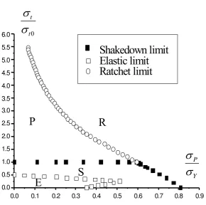
Figure 6 shows the shakedown and ratchet boundaries for the problem, using the methods described in (Ponter and Chen, 2001; Chen and Ponter, 2001b). Note that σ_t₀ =2σ_y is the value of σ_t at the reverse plasticity shakedown limit. In this paper we use the perfect plasticity material model.

(18)

varying strain Δεrp

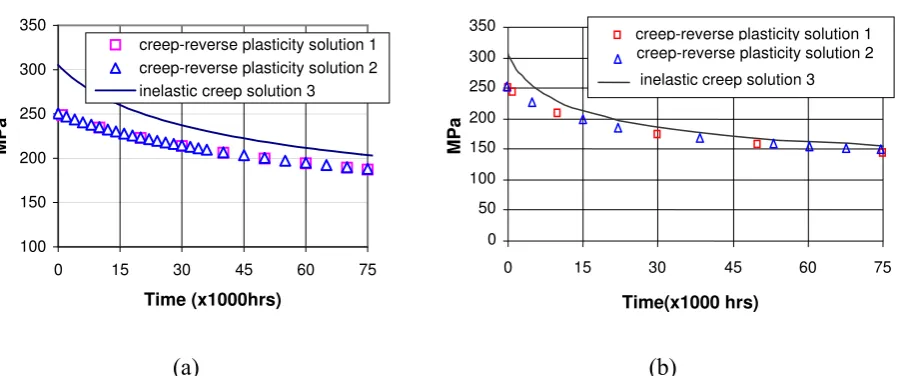
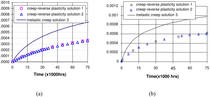
, including creep relaxation is the summation of varying plastic strain Δεp and accumulated creep strain Δεc. Fig. 7, 8 and 9 present the calculated maximum von Mises creep flow stress, the maximum von Mises creep strain and the elastic follow-up factor Z with creep dwell time for equation (29A) and (29B), respectively. Although the rate of relaxation and the growth of strain differ, the Z values are very similar, Figures 9a and 9b, with lower values for the temperature dependent case. Solutions for Method 1 and 2 are coincident, indicating that the assumption in Method 1, that Z remains constant during the relaxation process, is acceptable. The results from Method 3 also have a good agreement with those from Method 1 and 2. This numerical fact verifies the applicability of the proposed creep-reverse plasticity solution methods 1 and 2 in the paper as well as the monotonic creep computation method 3 based upon rapid cycle creep solutions.

For load case 2, the applied load domain is in the elastic shakedown region, where 0

, 0 Δ = =

Δεp ρp

(19)

8. Discussions

Although the solutions for method 1 and 2 are near identical, they differ from those of method 3 that tends to give higher values of Z, particular in the case of loading below the shakedown limit. (Boulbibane and Ponter, 2002) have noted that this method tends to give conservative values of Z although for a different constitutive equation and loading history.

Methods 1 and 2 use different material assumptions to method 3. In method 3 the Bailey-Orowan model is used for the rapid cycle solution. The Bailey-Bailey-Orowan model produces a different start-of-dwell stress below the shakedown limit, but a value that is very similar to Methods 1 and 2 in excess of shakedown where the initial stress needs to satisfy yield in all cases. If the applied load domain exceeds elastic shakedown and is in the reverse plasticity region, the start-of-dwell stress using rapid cycle solutions by Bailey-Orowan model (method 3) is consistent with the initial flow stress by the proposed methods 1 and 2 because in all cases the initial elastic stresses associated with the applied cyclic loads were amended by a varying residual stress field associated with the reverse plasticity mechanism. Both the maximum start-of-dwell stress and initial maximum flow stress equal to the yield stress of the material. Hence for load case 1 in this paper, where the applied load domain induces the reverse plasticity mechanism, the creep-reverse plasticity solution methods 1 and 2 nearly produce the same results as the monotonic creep computation method 3.

(20)

The elastic follow-up factor Z is assumed reasonably to be a constant when the creep relaxation is dominated by the thermal stress. The further investigations to the effects of the dominant mechanical stress on the creep will be performed in the future paper.

In order to simplify the formulations, the Norton’s law is adopted in equation (16) of the paper. Normally, the adoption of Norton’s law for creep may cause misevaluation of creep damage during dwell time due to the neglect of transient creep. In order to overcome this, in the paper, we have considered the transient creep by fitting the transient creep data into the Norton’s law, i.e. the creep material data in the Norton’s law (29B) have already considered the effect of the transient creep, which are different with those for the steady state creep.

Only two load instances are considered in this paper for method 1 and 2, although in method 3 multi-load extremes are adopted. For a general case of arbitrary loading, a more complicated method is being developed and will be presented in the future paper.

9. Conclusions

(21)

sensitive to the assumptions made in these particular calculations. The overall implication is that the particular assumptions made in Method 1 are probably acceptable for a general purpose technique for the evaluation of creep/ fatigue interaction. These methods were devised with the needs of the life assessment method R5 particularly in mind, although the approach to creep/fatigue interaction is similar in other life assessment procedures.

The completion of Method 1 involves two stages. The first stage involves the evaluation of the plastic strain amplitude, assuming no creep occurs during the dwell period. This involves the solution of a sequence of linear problems to convergence. The number of iterations required varies with the convergence criterion, but the order of thirty iterations is usually sufficient. If the load level is below the shakedown limit this stage becomes unnecessary. Although the solutions in this paper assume perfect plasticity, cyclic hardening may be included without any increase in the computational effort. The second stage involves a calculation which is computationally similar to the first stage and the same effort is required. Hence a complete solution for a particular case would require the solution of about sixty linear initial strain problems.

(22)

Appendix 1: Elastic Follow-up factor Z for proportional relaxation

Consider the case when a structure with volume V possesses a residual stress field σij0 at time 0

=

t . For t>0, creep occurs where the total strain rate ε&_ij is given by,

(

0

)

1 0 0 , 2 3 2 1 T T G ij n n ij

ij _σ σ σ

ε σ μ

ε_&′ = _&′ + & − ′

A1.1

kk kk

Kσ

ε& = 1 & A1.2

(

)

⎭ ⎬ ⎫ ⎩ ⎨ ⎧ − − = 0 0 1 1 exp , T T R Q T T G

where ε&0denotes the uniaxial creep rate corresponding to an uniaxial stress σ0 at a temperature

0

T . The creep behaviour is governed by the creep index n and the creep activation energy Q.

Rdenotes the universal gas constant and (μ,K) denote the linear elastic shear and bulk moduli, assumed temperature independent. Consider a history of stress relaxation for t>0,

) ( )

(t _ij0f t

ij σ

σ = A1.3

As 0 ij

σ is a residual stress field,

0 0 ₌

∫

ij

Vσijε& A1.4

and hence, from A1.1 and A1.2,

) ( )

( 2

0= Uf& t +D&Cfn t

A1.5 where Udenotes the total elastic complementary strain energy at t=0,

dV K

U

V ij ij kk

∫

_⎭⎬⎫ ⎩ ⎨ ⎧ + ′ ′

= ₀ ₀ 1 ₀2

2 1 2

1 _σ _σ _σ

μ A1.6

(23)

GdV D ij n V n C ) ( 0 1 0

0σ σ σ

ε +

∫

= &

& _A1.7

Integrating equation (A1.5) we obtain, assuming n>1,

(

)

(

)

( 1)

1 1 1 1 ) ( − − + = n t n t f

α where U D&C =

α A1.8

With f(t) known, the elastic follow-up factor may be computed for any position in the structure. From A1.3 and A1.1,

) ( )

(t σ0f t

σ = , t f dt

t n n C

∫

= 0 0 0 0 ) ( σ σ ε

ε & A1.9

where σo denotes the effective stress at t=0 and εC the effective creep strain accumulated since 0t= . The effective Young’s modulus during stress relation is, therefore given by,

(

)

C

eff f t

Z E E ε σ σ ν ν ) ( 1 ) 1 ( 2 3 ) 1 ( 2

3 0₋ 0

= +

=

+ = 1

0 0 0 − n n σ ε σ α

& A1.10

The maximum value of Z generally occurs in the location where σ0 =σ0max at the position of maximum effective stress at t=0. We will assume that T =T₀ at the same location and adjust ε&₀ accordingly. From A1.6, A1.7 and A1.8, A1.10 may now be expressed in the following form;

c D U Z _~ ~ 2 &

= A1.11

where D~&C and U~ are the creep energy dissipation and complementary elastic strain energy normalised with respect to the maximum effective stress σ0max,

GdV D n V ij C 1 max 0 0 ) ( ~ +

∫

_⎪⎭⎪⎬⎫ ⎪⎩ ⎪ ⎨ ⎧ = σ σ σ

& _A1.12

(24)

dV

E

K U

V

kk ij

ij

∫

₊ ⎭⎬

⎫ ⎩

⎨ ⎧

+ ′ ′

=

2 max 0

2 0 0

0

) ( 3

) 1 ( 2

1 2

1

2 1 ~

σ ν

σ σ

σ μ

A1.13

Equations A1.11, A1.12 and A1.13, provide valuable insight into the dependence of Z on the characteristics of the problem.

a) Z is independent of the overall magnitude of the stress distribution, i.e. the stress distribution σ_ij0 and Xσ_ij0, where X is a constant, will give identical values of Z. However Z is strongly dependent on the distribution of the stress.

b) Z is independent of Young’s modulus E, but weakly dependent on Poisson’s ratio v. c) Z is independent of the overall creep rate, but dependent on the creep index n, the

distribution of G.

Appendix 2: Z for beam problems

For a mean subjected to loads perpendicular to it’s length, a similar analysis may be carried out when the total curviture rate

) , ( 0 0

0

T T G M M EI

M n

n κ

κ&= & + & A2.1

where κ&₀ is the curvature rate occurring at temperature T₀ and moment M₀. Again, for a moment history of the form M(x,t)=M0(x)f(t), the elastic follow-up factor Z is given by,

c

D U

Z _~

~ 2

&

= A2.2

(25)

Gdx M M D n l 1 0 max 0 0 ~ +

∫

_⎭⎬⎫ ⎩ ⎨ ⎧ =

& _A2.3

and dx M M U l o 2 0 max 0 2 1 ~

∫

_⎭⎬⎫ ⎩ ⎨ ⎧

= A2.4

Consider the following special cases,

Case 1: Cantilever beam of length L, subjected to a fixed lateral end displacement and uniform temperature (Figure A1).

) ( 1

) ,

( max f t

L x M t x M ⎟ ⎠ ⎞ ⎜ ⎝ ⎛ −

= A2.5

where )Mmax =M(0,0 .

3 2 1 1 0 1 0 2 + = ⎟ ⎠ ⎞ ⎜ ⎝ ⎛ − ⎟ ⎠ ⎞ ⎜ ⎝ ⎛ − =

∫

+ n dx L x dx L x Z L n L A2.6

Case 2: Cantilever beam of length L, subjected to a fixed lateral end displacement and uniform temperature in 0≤x≤βL where G=1. In βL≤x≤L, G=0.(Figure A1)

(

)

(

2

)

0 1 0 2 1 1 3 2 1 1 + + ₋ ₋ + = ⎟ ⎠ ⎞ ⎜ ⎝ ⎛ − ⎟ ⎠ ⎞ ⎜ ⎝ ⎛ − =

∫

n L n L n dx L x dx L x Z β

β A2.7

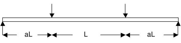
Case 3 and 4: Beam of length (2α+1

)

L under four point bending and uniform temperature

(26)

At t=0 displacements are assigned at the four loading points so that the moment in the central section is constant. These displacements are then held constant. For Case 3 we assume that G=1 for the entire beam giving,

(

)

(

2 3

)(

2

)

2 2 3

+ +

+ + =

n n Z

α α

A2.8

If we now assume, Case 4, that creep occurs only in the central section and no creep occurs in the outer sections,

⎟ ⎠ ⎞ ⎜

⎝ ⎛ ₊

= 1

3 2α

Z A2.9

and Z is independent of n.

Acknowledgements

The authors gratefully acknowledge the support of the Engineering and Physical Sciences Research Council of the United Kingdom, British Energy Ltd and the University of the Leicester during the course of this work.

References

ABAQUS, 2001. User’s Manual, Version 6.2.

Ainsworth, R.A. (editor), 2003. R5: Assessment Procedure for the High Temperature Response of Structures. Issue 3, British Energy Generation Ltd.

(27)

Boulbibane, M., Ponter, A. R. S., 2002. A Method for the Evaluation of Design Limits for Structural Materials in a Cyclic State of Creep. European Journal of Mechanics, A/Solids, 21 (6), 899-914.

Boyle, J.T., Hamilton, R., Shi, J., Mackenzie, D., 1997. Simple method of calculating lower-bound limit loads for axisymmetric thin shells.Journal of Pressure Vessel Tech 119, 236-242. Chen, H. F., Engelhardt, M.J., Ponter, A.R.S., 2003. Linear matching method for creep rupture

assessment. International Journal of Pressure Vessels and Piping, Vol. 80, 213-220.

Chen, H. F., Liu, Y. H., Cen, Z. Z., Xu, B. Y., 1999. On the Solution of Limit Load and Reference Stress of 3-D Structures under Multi-loading Systems. Engineering Structures, Vol. 21, 530-537.

Chen, H. F., Ponter, A.R.S., 2001a. Shakedown and Limit Analyses for 3-D Structures Using the Linear Matching Method. International Journal of Pressure Vessels and Piping, Vol. 78(6), 443-451.

Chen, H. F., Ponter, A.R.S., 2001b. A Method for the Evaluation of a Ratchet Limit and the Amplitude of Plastic Strain for Bodies Subjected to Cyclic Loading. European Journal of Mechanics, A/Solids, 20 (4), 555-571.

Corradi, L., Zavelani, A., 1974. A linear programming approach to shakedown analysis of structures. Comput. Methods Appl. Mech. Engrg., Vol. 3, 37-53.

Engelhardt, M., 1999. Computational modelling of Shakedown. PhD thesis, University of Leicester.

(28)

Hubel, H., Zeibig, H., 1996. State of the art of simplified methods to account for elastic follow-up in creep. EUR 16556EN, Directorate-General Science, Research and Development, Office of Official Publication of the European Communities, ISBN 92-827-5009-4.

Mackenzie, D., Boyle, J. T., Hamilton, R., Shi, J., 1996. Elastic compensation method in shell-based design by analysis. Proceedings of the 1996 ASME Pressure Vessels and Piping Conference, Vol. 338, 203-208.

Maier, G., 1977. Mathematical programming methods for deformation analysis at plastic collapse. Computers and Structures, Vol. 7, 599-612.

Ponter, A.R.S., Chen, H. F., 2001. A minimum theorem for cyclic load in excess of shakedown, with application to the evaluation of a ratchet limit. European Journal of Mechanics, A/Solids, 20 (4), 539-553.

Ponter, A.R.S., Cocks, A.C.F., 1994. Computation of shakedown limits for structural components (Brussels Diagram)-Part 2-The creep range. Nuclear Science and Technology, European Commission, Report No. EUR 15682EN, Luxembourg.

Ponter, A. R. S., Engelhardt, M., 2000. Shakedown limits for a general yield condition: implementation and application for a Von Mises yield condition. European Journal of Mechanics - A/Solids, Volume 19, Issue 3, 423-445.

(29)

Caption

Table 1. Variation of the Elastic Follow-up factor Z with creep index n for the beam problems of Figure A1 and A2

Table 2. The definition of load domains for the holed plate

Fig. 1 The load history with two distinct extremes to the elastic solution Fig. 2 Creep-reverse plasticity mechanisms by steady cyclic loads

Fig. 3 Schematic representation of the quantities for (a) pure reverse plasticity mechanism and (b) creep-reverse plasticity mechanism

Fig. 4 The flow chart for creep-reverse plasticity solution method

Fig. 5 The geometry of the holed plate subjected to varying thermal loads and its finite element mesh (D/L=0.2), the yield stress σY =360MPa, the elastic modulus E =208GPa

Fig. 6 The elastic, shakedown, reverse plasticity and ratchet region for the holed plate with constant mechanical and varying thermal loading

Fig. 7 The maximum flow stress with creep dwell time for a holed plate subjected to varying thermal loads from 0 to 1.5σ_t₀ (a)with constant ε&₀ using eqn (27A); (b) with temperature-dependent ε&₀ using eqn (27B)

(30)

Fig. 9 The elastic follow-up factor Z with creep dwell time for a holed plate subjected to varying thermal loads from 0 to 1.5σ_t₀ (a) with constant ε&₀ using eqn (27A); (b) with temperature-dependent ε&₀ using eqn (27B)

Fig. 10 The maximum flow stress with creep dwell time for a holed plate subjected to varying thermal loads from 0 to 0.8σ_t₀ (a) with constant ε&₀ using eqn (27A); (b) with temperature-dependent ε&0 using eqn (27B)

Fig. 11 The maximum creep strain with creep dwell time for a holed plate subjected to varying thermal loads from 0 to 0.8 σt0 (a) with constant ε&0 using eqn (27A); (b) with temperature-dependent ε&₀ using eqn (27B)

Fig. 12 The elastic follow-up factor Z with creep dwell time for a holed plate subjected to varying thermal loads from 0 to 0.8 σ_t₀ (a) with constant ε&₀ using eqn (27A); (b) with temperature-dependent ε&₀ using eqn (27B)

Fig. A1 Configuration for Case 1 and 2

(31)

[image:31.595.43.495.209.301.2]

Table 1 Variation of the Elastic Follow-up factor Z with creep index n for the beam

problems of Figure A1 and A2

Case 1 – Propped cantilever, creep over entire length Case 2a – Propped cantilever, creep over 0.5 of length Case 2b – Propped cantilever, creep over 0.1 of length

Case 3- Beam under four point bending, creep over entire length

Case 4 – Beam under four point bending, creep over constant moment section

n 1 3 5 7 n→∞

Case 1 1 1.67 2.33 3.00 ∞

Case 2a,

β

=0.5 1.14 1.72 2.33 3.01 ∞

Case 2b,

β

=0.1 3.69 4.07 4.47 4.90 ∞

Case 3, α =1 1 1.19 1.30 1.36 1.67

Case 4, α =1 1.67 1.67 1.67 1.67 1.67

Table 2 The definition of load domains for the holed plate

Case The cyclic thermal load Δθ Δεp _Δεrp

Case 1 1.5σ_t₀ →0→1.5σ_t₀ →0→1.5σ_t₀L 3

10 869 .

2 × − Δεp +Δεc(t)

Case 2 0.8σt0 →0→0.8σt0 →0→0.8σt0L 0 (t) c

ε

[image:31.595.79.486.467.559.2]

(32)

[image:32.595.107.483.57.171.2]

Fig. 1 The load history with two distinct extremes to the elastic solution

(a) Δρ p ≠ 0, Δε p ≠ 0_(b)

0 ,

0 Δ = =

[image:32.595.116.473.253.463.2]

Δρ p ε p

Fig. 2 Creep-reverse plasticity mechanisms by steady cyclic loads

(a) (b)

Fig. 3 Schematic representation of the quantities for (a) pure reverse plasticity

y

σ

-

σ

_y 0

Strain ε Stress σ

c c _ε ρ Δ Δ , c rp c

rp ρ ε ε

ρ =Δ Δ =Δ

Δ ,

y

σ

-

σ

y

0

Strain ε Stress σ

p p ε ρ Δ Δ , c c ε ρ Δ Δ , c p rp c p

rp _ρ _ρ _ε _ε _ε

ρ = Δ +Δ Δ = Δ +Δ

Δ , A B C D p ρ Δ p ε Δ c p ε

ε −Δ Δ −

c

p ρ

ρ −Δ Δ − 1 σ y σ σ = 2 σ c ρ Δ c ε Δ c σ σ = ∆t ∆t ∆t

t1 t2 t

θ

_∆

t

t1 t2 t

P

A′

-Δεp

p ρ Δ p ε Δ

-Δρp

[image:32.595.93.442.542.712.2]

(33)

[image:33.595.89.513.61.652.2]

Fig. 4 The flow chart for creep-reverse plasticity solution method Elastic analysis

Elastic & plastic shakedown analysis (reverse plasticity limit, ratchet limit)

Reverse plasticity appears in the body?

Yes

Reverse plasticity solution

(varying residual stress Δ

ρ

p, varying plastic strain Δ

ε

p) No

Creep-reverse plasticity solution (varying residual stress Δ

ρ

c

, varying creep strain Δ

ε

c

, the flow stress

σ

_f and elastic follow-up factor Z with dwell time)

Creep endurance limit D_c from above

data, hence N₀∗

c p

rp

ε

=Δ +Δ

Δ

for low cycle fatigue evaluation (fatigue cycles to failure N₀)

Calculate total damage

(34)

[image:34.595.368.524.57.196.2]

Fig. 5 The geometry of the holed plate subjected to varying thermal loads and its finite

element mesh (D/L=0.2), the yield stress

σ

_Y =360MPa, the elastic modulus E=208GPa

0.0 0.1 0.2 0.3 0.4 0.5 0.6 0.7 0.8 0.9

0.0 0.5 1.0 1.5 2.0 2.5 3.0 3.5 4.0 4.5 5.0 5.5 6.0

Shakedown limit

Elastic limit

Ratchet limit

0

t t

σ

Y P

σ

P

R

[image:34.595.153.444.385.673.2]

S

E

Fig. 6 The elastic, shakedown, reverse plasticity and ratchet region for the holed plate with constant mechanical and varying thermal loading

D L

y

x

θ

₀ +Δ

0

θ

0

(35)

0 50 100 150 200 250 300 350 400

0 10 20 30 40 50

Time (hrs)

MPa creep-reverse plasticity solution 1

creep-reverse plasticity solution 2

inelastic creep solution 3

[image:35.595.81.512.62.258.2]

(a) (b)

Fig. 7 The maximum flow stress with creep dwell time for a holed plate subjected to

varying thermal loads from 0 to 1.5

σ

_t₀ (a) with constant

ε

&₀ using eqn (27A); (b)with

temperature-dependent

ε

&₀ using eqn (27B)

0.0000 0.0002 0.0004 0.0006 0.0008 0.0010 0.0012

0 10 20 30 40 50

Time (hrs)

creep-reverse plasticity solution 1 creep-reverse plasticity solution 2 inelastic creep solution 3

(a) (b)

Fig. 8 The maximum creep strain with creep dwell time for a holed plate subjected to

σ

_t₀ (a)with constant

ε

&₀ using eqn (27A); (b) with

ε

0 50 100 150 200 250 300 350 400

0 10 20 30 40 50

Time( hrs)

MPa _{creep-reverse plasticity solution 1}

creep-reverse plasticity solution 2 inelastic creep solution 3

0 0.0002 0.0004 0.0006 0.0008 0.001 0.0012 0.0014

0 10 20 30 40 50

creep-reverse plasticity solution 1 creep-reverse plasticity solution 2

[image:35.595.102.516.463.659.2]

(36)

0 0.5 1 1.5 2 2.5 3

0 10 20 30 40 50

Time (hrs)

[image:36.595.81.526.104.291.2]

(a) (b)

Fig. 9 The elastic follow-up factor Z with creep dwell time for a holed plate subjected to

σ

_t₀ (a)with constant

ε

&₀ using eqn (27A); (b) with

ε

100 150 200 250 300 350

0 15 30 45 60 75

Time (x1000hrs)

MPa

(a) (b)

Fig. 10 The maximum flow stress with creep dwell time for a holed plate subjected to

σ

t₀ (a) with constant

ε

&0 using eqn (27A); (b) with

ε

0 0.4 0.8 1.2 1.6 2 2.4

0 10 20 30 40 50

Time( hrs)

inelastic creep solution 3 creep-reverse plasticity solution 2 creep-reverse plasticity solution 1

0 50 100 150 200 250 300 350

0 15 30 45 60 75

Time(x1000 hrs)

MPa

[image:36.595.85.535.481.669.2]

(37)

0.0000 0.0001 0.0002 0.0003 0.0004 0.0005 0.0006 0.0007 0.0008 0.0009 0.0010

0 15 30 45 60 75

Time (x1000hrs)

[image:37.595.95.539.85.289.2]

(a) (b)

Fig. 11 The maximum creep strain with creep dwell time for a holed plate subjected to

σ

ε

&₀ using eqn (27A) ; (b) with

ε

0 0.4 0.8 1.2 1.6 2

0 15 30 45 60 75

Time (x1000hrs)

(a) (b)

Fig. 12 The elastic follow-up factor Z with creep dwell time for a holed plate subjected

to varying thermal loads from 0 to 0.8

σ

ε

&₀ using eqn (27A) ; (b)

with temperature-dependent

ε

0 0.0002 0.0004 0.0006 0.0008 0.001 0.0012

0 15 30 45 60 75

Time(x1000 hrs) inelastic creep solution 3 creep-reverse plasticity solution 1 creep-reverse plasticity solution 2

0 0.4 0.8 1.2 1.6 2

0 15 30 45 60 75

Time(x1000 hrs)

[image:37.595.100.526.441.629.2]

(38)

x

L

[image:38.595.141.451.146.248.2]

d

Figure A1 Configuration for Case 1 and 2

aL aL L

[image:38.595.144.453.439.513.2]