Recursive estimation in the identification of air pollution models

IDENTIFICATION OF AIR POLLUTION M ODELS

by

Lloyd Paul Steele

A thesis submitted to the

Australian National University

for the degree of Doctor of Philosophy

PREFACE

Part of the research reported in Chapter 5 was carried out jointly

with Dr A.J. Jakeman and Professor P.C. Young. The results of this work

have been published*, and frequently the text of this paper has been

closely followed. Some sections of Chapters 4 and 6 are based on work

undertaken with Dr Jakeman and partly reported in Steele and Jakeman

(1980). The remainder of this thesis, except where otherwise

acknowledged in the text, represents the original research of the

author.

Jakeman, A.J., Steele, L.P. and Young, P.C., 'Instrumental

Variable Algorithms for Multiple Input Systems Described by

Multiple Transfer Functions.' IEEE Transactions on Systems, Man

I would like to thank my supervisors Professor Peter Young and Dr

Anthony Jakeman for their advice and the interest they have shown in

this work.

I am also grateful to the following for their assistance: to Dr

Neil Daly of the Australian National University for permission to carry

out the experiments on the carbon monoxide analyser, the results of

which are reported in Chapter 4, and to Mr Anthony Chetcuti for his

assistance in setting up the equipment for some of these experiments;

to Dr Bob Spear of the University of California at Berkeley for

supplying the ozone data used in Chapter 5; to Mr Bill Danaher of the

National Capital Development Commission in Canberra for supplying the

traffic data used in Chapter 6; and finally to Dr Glenn Johnson of

Macquarie University for permission to perform experiments on the

Macquarie Urban Air Quality model, the results of which are reported in

Chapter 7.

I would also like to thank Cherie Cromwell for her fast and

accurate typing and Wendy Steele for her careful proof-reading of the

final draft. Special thanks must go to Ian McLean for his timely

encouragement and support during the writing of this thesis.

This work was made possible by the financial support of a

ABSTRACT

This thesis is an inquiry into the use of recursive estimation

procedures in both modeling and measurement of air pollution. Recursive

estimation methods were selected for investigation partly because little

use has been made of them in air pollution modeling, but primarily for

the reason that they offered a promising additional method of time

series analysis. In particular the presence of parameter variation in

time series models in readily determined, thus assisting the choice of

appropriate structures for air pollution models. The modeling

undertaken in this thesis has as its principal objective the derivation

of simple and operational models for use in air quality management.

Since the management of air quality is usually based upon a model of air

pollution, such management should be assisted by improved measurement of

ambient pollutant levels. A possible added benefit of these improved

measurements is that they may enable a better discrimination between

alternative air pollution models.

The first three chapters constitute a framework within which the

subsequent empirical chapters are appropriately located. A broad

perspective of the modeling of complex systems in general is offered in

Chapter 1. In Chapter 2 the focus is narrowed to models of air

pollution - the primary concern of the thesis. The following chapter

introduces the recursive estimation techniques which were employed

extensively in later chapters. A series of inquiries into aspects of

both air pollution monitoring and modeling are then reported. In

Chapter 4 transfer function models of a continuous air pollution

analyser were secured and employed in the derivation of robust input

signal estimation algorithms. Then, in Chapter 5, estimates are made of

missing air pollution data using simple linear dynamic models. There

follows in Chapter 6 an attempt at developing a simple time series model

for carbon monoxide levels in an urban area. Finally in Chapter 7, an

investigation is reported into the dynamic properties of a deterministic

model for simulating urban air pollutant levels.

The results of the thesis may be summarised succinctly. Recursive

estimation methods have been found both appropriate and effective at

models of continuous air pollution analysers; in the estimation of

’true’ input pollutant concentration; in examining the dynamic

properties of a deterministic simulation model for urban air pollutant

levels; and in the analysis of air pollution and meteorological data.

Additionally, it is successfully demonstrated that simple linear dynamic

models yield satisfactory estimates of data missing from time series of

air pollutant levels. Finally, recursive algorithms are developed for

estimating the parameters in a particular class of linear dynamic

Table of Contents

Preface ii

Acknowledgements ill

Abstract iv

Chapter One MODELING COMPLEX SYSTEMS - AN OVERVIEW

1.1 Introduction 1

1.2 Complex systems and 'badly defined' systems 2

1.3 Modeling 'badly defined' systems 3

1.4 The model building procedure and the model form 5

1.5 Identification, estimation and validation 8

1.6 Thesis outline 10

Chapter Two INTRODUCTION TO THE AIR POLLUTION PROBLEM

AND AIR POLLUTION MODELING

2.1 A brief history 12

2.2 Air quality 15

2.3 Measuring and monitoring air pollution 17

2.4 Urban air pollution modeling 19

2.4.1 Mass conservation models 20

2.4.2 Gaussian diffusion models 26

2.4.3 Physically based stochastic dispersion

models 28

2.4.4 Statistical models and time series

models 30

Chapter Three RECURSIVE METHODS FOR THE IDENTIFICATION AND

ESTIMATION OF TIME SERIES MODELS

3.1 Introduction 35

3.2 Recursive estimation 35

3.3 Dynamic time series models 41

3.4 Estimation of time varying parameters 49

A CONTINUOUS AIR POLLUTION ANALYSER

4.1 Introduction 57

4.2 Experimental procedure 58

4.3 Identification of model order and estimation of

model parameters 62

4.4 Dynamic check of the linearity of the analyser 66

4.5 Choice of input signals for optimal estimation 71

4.6 Effect of sample gas flow rate on the dynamics of

the analyser 75

4.7 Continuous time models and the analyser's frequency

response 75

4.8 Input estimation 81

4.9 Demonstration of the input estimation algorithms 85

4.10 Conclusion 92

Chapter Five SIMPLE LINEAR DYNAMIC MODELS FOR ESTIMATING

MISSING AIR POLLUTION DATA

5.1 Introduction 93

5.2 Derivation of the instrumental variable methods 94

5.3 Implementation of the algorithms 99

5.4 Simulation studies 103

5.5 Discussion of the simulation results 109

5.6 Estimating missing ozone data 123

5.6.1 Simple SISO models 126

5.6.2 MISO models 130

5.6.3 SISO models using 'averaged' inputs 132

5.6.4 Direct evaluation of the SISO model

forecasts 134

5.7 Conclusions 135

Chapter Six RECURSIVE METHODS FOR MODELING CARBON MONOXIDE

IN AN URBAN AREA

6.1 Introduction 137

6.2 Review of models for describing vehicle pollution

from roadways 138

6.4 Initial modeling 145

6.5 Modeling the wind effects 148

6.5.1 Analysis of wind speed and direction 148

6.5.2 Evaluation of Hanna's model 154

6.5.3 Modeling wind speed and direction 156

6.6 Discussion of results 159

Chapter Seven INVESTIGATION OF THE DYNAMICS OF A DETERMINISTIC

AIR POLLUTION MODEL

7.1 Introduction 167

7.2 The SAI model 168

7.3 The Macquarie Urban Air Quality (MUAQ) model 170

7.4 Experimental procedure 171

7.5 Initial results 175

7.6 Input-output modeling results 178

7.7 Discussion and conclusions 185

Chapter Eight SUMMARY AND CONCLUSIONS 190

Appendix 193

MODELING COMPLEX SYSTEMS - AN OVERVIEW

1.1 Introduction

The aim of this thesis is to demonstrate that for the purposes of

air quality management simple but effective dynamic air pollution

models may be obtained by a particular model building procedure based

upon recursive estimation methods. The models are simple in the sense

that they have few parameters, and they differ from many others in that

they are stochastic rather than deterministic. Often linear models are

found to be adequate, but even in cases where the overall model is

non-linear it is usually possible to separate it into linear and

non-linear components, so that the methods of linear systems analysis

may still be employed for the linear component.

The development of air pollution models was greatly spurred by

the United States Clean Air Act amendments of 1970, although

legislation to control air pollution had existed in several

industrialised countries prior to that time (Persson, 1977). The

crucial aspect of the amendments was the adoption of an air quality

management approach to air pollution control (de Nevers et al., 1977),

an approach which was based on the specification of a set of national

ambient air quality standards. The three basic requirements of an air

quality management approach are knowledge of pollutant emissions, air

quality monitoring data and air pollution models. Many countries have

now adopted some variation of this approach to air pollution control

(see, for example, Campbell and Heath, 1977).

It has been recognised for some time (for example, Stern, 1970)

that air pollution models may serve two quite diverse purposes: they

assist our understanding of the physical nature of the atmosphere;

alternatively, they may be used as aids in decision making in air

pollution control and city and regional planning. It is the use of

models for this latter purpose which is of interest in this thesis.

The development of models suitable for the purposes of air

quality management has proved very difficult, and presumably as a

(see, for example, Hanna, 1975). Scorer (1976) concludes that the

problems encountered in air pollution modeling lie primarily in the

complexity of atmospheric behaviour, and also that the limitations of

the models greatly restrict the usefulness of the air quality

management approach to air pollution control. However, it is a central

contention of this thesis that the pessimism of Scorer is not

warranted. By placing air pollution modeling in the wider context of

modeling complex systems it is argued here that there exists

considerable scope for improving the performance of air pollution

models, and hence the usefulness of the air quality management approach

to controlling atmospheric pollution.

1.2 Complex Systems and fBadly Defined’ Systems

Simon (1965) defines a complex system as one 'made up of a large

number of parts that interact in a non-simple way. In such systems,

the whole is more than the sum of the parts, not in an ultimate,

metaphysical sense, but in the important pragmatic sense that, given

the properties of the parts and the laws of their interaction, it is

not a trivial matter to infer the properties of the whole.' Ecosystems

are complex in this sense. For example, if the respiration of each

organism inhabiting an ecosystem was measured by placing it into a

respirometer, the sum of the respiration of individuals would not equal

that of the whole ecosystem measured by placing it in a single giant

respirometer. Those characteristics which arise from such

non-additivity of the component parts are called emergent properties

(Perkins, 1975).

Related to the concept of complexity is that of a 'badly defined'

system (Young, 1978). Poor understanding of a system may be due either

to its complexity or to a number of other factors such as (i) the

difficulty or impossibility of performing planned experiments, (ii) the

uncertain quality of measurements drawn from the system, and (iii) the

limited resources available for making comprehensive measurements of

the system. For instance, macroeconomic systems may be considered to

be 'badly defined' because they are complex, subject to the vagaries of

human behaviour, and plagued by the three factors listed above.

We would contend that for the purposes of modeling for air

underlie the transport, diffusion and transformation of air pollutants

are not conceptually complex, urban airsheds are characterised by

conditions (i) to (iii). First, planned experiments in the form of

atmospheric tracer experiments are possible (for example, McElroy, 1969

and Lange, 1978) but are difficult and costly. Second, measurements of

air pollution levels may be uncertain because the method chosen may not

be completely specific for a particular pollutant (for example, Winer

et al., 1974), there may be unrecognised calibration errors (for

example, see Pitts, 1976), or the location of monitoring stations may

not be appropriate to the purposes of the measurements (for example,

Ludwig and Shelar, 1978). Moreover, estimates of pollutant emissions

are notoriously uncertain, particularly those of motor vehicle

emissions (see, for example, Bullin et al., 1980). The third

condition, that usually only limited resources are available for

measurements of an urban airshed, is perhaps best illustrated by

reference to a well known exception, namely, the ambitious St. Louis

regional air pollution study (RAPS) in which an extensive network of

monitoring stations was established (see, for example, Pooler, 1974).

Finally, additional complexity is introduced because dispersion of

pollutants in the airshed may be altered due to changes in the surface

roughness and as a consequence of the development of urban heat islands

(see, for example, Kopec, 1970).

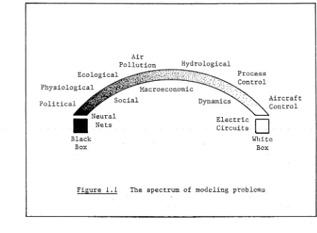
1.3 Modeling 'Badly Defined' Systems

Vemuri (1978) has suggested that the range of problems

encountered in the mathematical modeling of complex or 'badly defined’

systems can be shown diagrammatically by means of a spectrum with

'black box' modeling at one extreme and 'white box' modeling at the

other. Some additions have been made to his diagram which is shown as

Figure 1.1. In pure black box modeling there is no explicit knowledge

of the processes occurring in the system and only the input(s) and

output(s) may be observed. By contrast, in pure white box modeling,

there is complete knowledge of the detailed workings of the system.

These two extremes are useful abstractions since there inevitably

exists some a priori knowledge of a system before attempts are made to

construct a mathematical model of it. t

t

Air

Pollution Hydrological

Process Control Ecological

Physiological _{Macroeconomic}

Aircraf t Control

Social Dynamics

Political

Neural

Nets Electric

Circuits

Black White

Box

Figure 1.1 The spectrum of modeling problems

Modeling ’badly defined’ systems is an inherently difficult task.

To illustrate, reference will be made to certain crucial problems with

the well-known global models, World2 of Forrester (1971) and World3 of

Meadows et a l . (1972). Thissen (1978), in concluding his comprehensive

analysis of the World3 model, found that 'each specific type of

behaviour of World3 appears to be primarily determined by only a

fraction of all the assumptions and equations. ... The model

builders. . . have spent needless amounts of time and energy on the

formulation and quantification of equations that, in fact, do not

matter at all as far as overall behaviour and conclusions are

concerned.’ More importantly, Thissen argues that ’model analyses

ought to be performed during the model construction phase in order to

know better on what to focus attention. ... Only thus can it be

determined which model parts and what circumstances deserve close

attention, and what can be ignored in the light of the goals set to the

study as a whole.’

The importance of clearly specified goals prior to modeling

’badly defined’ dynamic systems has also been stressed by Young (1978,

1980a). He discusses the relative merits of reductionist and holistic

restraints on the way measurements of the components are made and

utilised. His emphasis on dynamic systems is important because

methodologies such as regression analysis, which are appropriate for

the analysis of static systems, may not be applicable to dynamic

systems (see Young, 1968). Some models of ’badly defined' dynamic

systems are specifically designed for control and management

applications. By such a specification of objectives, and by use of the

concept of modal dominance in a complex system, Young (1978) argues

that 'the model structure should be chosen so that it 'explains' the

data in the simplest, physically meaningful manner possible, and then

only to a degree which is defined carefully in relation to the

uncertainty on the data.' Before turning in the next section to a

detailed consideration of Young's model building procedure, some

emphasis must be given to the points raised in this and previous

paragraphs.

The position adopted in this thesis is in sympathy with these

above views, namely that in modeling complex or 'badly defined' dynamic

systems for control and management purposes, the principle of Occam's

razor should apply. Thus it is argued that air pollution models for

such management purposes should incorporate only as much complexity and

data intensiveness as is strictly necessary to achieve consistency with

the available air pollution measurements and the goals of the modeling.

Similar views have been expressed by Johnson (1979a), Phadke et al.,

(1976) and, perhaps most convincingly, by Gifford and Hanna (1973) who

concluded that 'the detailed urban diffusion models developed so far

have the property that they generate much more pollution variability

than is actually observed to occur. This seems to us to be a strong

argument for the use of simpler models.'

1.4 The Model Building Procedure and the Model Form

The model building procedure suggested by Young (1978, 1980a),

and adopted in this thesis, is basically heuristic but has the

advantage of being comprehensive. It consists of four major stages

-(i) the formulation of plausible a_ priori model structures,

possibly by resort to speculative simulation modeling;

parameterised model structures on the basis of the

results obtained in the first stage, and in relation to

the objectives of the modeling;

(iii) the estimation of those parameters which characterise

the model structures eventually chosen; and

(iv) the conditional validation of the estimated models, as

implied by the failure to reject the models as reasonable

representations of the system's behaviour.

In the first stage, speculative simulation models may be

formulated within a probabilistic context by defining the model

parameters in terms of statistical probability distributions (see, for

example, Hornberger and Spear, 1980; Spear and Hornberger, 1980; and

Humphries et al., 1981). The resultant ensemble of models may then be

investigated by use of Monte-Carlo simulation analysis in which the

model equations are solved repeatedly with the parameters specified by

sampling at random from their assumed parent probability distributions.

Such analysis may allow determination of those parameters which are

most important in giving rise to the observed behaviour in the system.

It is well known that the dominant factors in air pollution episodes

are the levels of pollutant emissions and certain meteorological

variables such as wind speed (see, for example, Hanna, 1971). As the

specific purpose of stage (i) is to determine just such basic

structural features of the system, this first stage of speculative

simulation modeling is not considered in this thesis. The subsequent

stages of the modeling procedure are discussed in the next section, but

it will first be helpful to explain briefly the philosophy underlying

this approach to modeling and to describe the preferred model form.

While recognising that ’badly defined’ dynamic systems will in

general exhibit both non-linear and non-stationary behaviour, Young

(1978) proposes that attention be limited to models designed for

control and management purposes and that initially the analysis be

restricted to small perturbation behaviour. A linear model is then

assumed to be applicable for describing the system behaviour. Whether

this assumption holds can be assessed directly because the recursive

estimation procedure allows examination of the model parameters to see

if they are time invariant. If this is found to be the case (as will

be seen for the models of a continuous air pollution analyser in

does not hold (as will be observed in Chapter 6 for a model of ambient

carbon monoxide levels), the non-linear characteristics of the system

will be revealed in the pattern of time variation of the model

parameters. This is the case because, in general, a non-linear system

may be described by a linear model with time-varying parameters. If

the causes of the time variation of the parameters can be identified it

may be possible to incorporate these causal factors directly into the

model. Hence the final model parameters become time invariant, once

again enabling them to be estimated by the methods of linear systems

analysis.

Young (1978) goes on to argue that, since in practice, the

observations of the system will be made in discrete time, and will be

characterised by stochastic effects, it is desirable to formulate a

discrete time, linear, stochastic model with parameters that may be

time variable to allow for any non-stationary behaviour. Furthermore,

since it is not usually possible to observe all the variables in a

system, he recommends the use of the concept of an observation space

which will have a dimension less than that of the full state space.

The model is then defined directly in the observation space and is

linear in the observations.

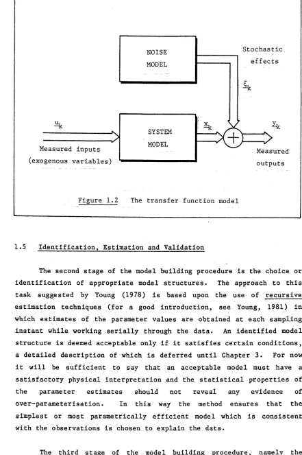
The discrete time series transfer function model suggested by Box

and Jenkins (1970) is the preferred model form since it is a stochastic

model which emphasises the separation of deterministic and stochastic

components. This model form is shown diagrammatically in Figure 1.2

for the general case with multiple measured inputs (denoted by the

vector u^) to the deterministic component of the model (the ’system'

model), and multiple outputs y^ which can only be measured in error.

The stochastic effects are assumed to be generated by the 'noise'

model, and since they are assumed to be additive to the deterministic

output x^ from the system model, this model form is sometimes

referred to as an errors-in-variables model (see Young, 1980b). The

particular terminology used in the formulation of such transfer

function models and the methods used for generating the stochastic

terms will be introduced in Chapter 3. We now turn to a

Stochastic

effects

Measured inputs

(exogenous variables)

Measured

outputs MODEL

NOISE

MODEL SYSTEM

Figure 1.2 The transfer function model

1.5 Identification, Estimation and Validation

The second stage of the model building procedure is the choice or

identification of appropriate model structures. The approach to this

task suggested by Young (1978) is based upon the use of recursive

estimation techniques (for a good introduction, see Young, 1981) in

which estimates of the parameter values are obtained at each sampling

instant while working serially through the data. An identified model

structure is deemed acceptable only if it satisfies certain conditions,

a detailed description of which is deferred until Chapter 3. For now

it will be sufficient to say that an acceptable model must have a

satisfactory physical interpretation and the statistical properties of

the parameter estimates should not reveal any evidence of

over-parameterisation. In this way the method ensures that the

simplest or most parametrically efficient model which is consistent

with the observations is chosen to explain the data.

The third stage of the model building procedure, namely the

estimation of the parameters in the identified model, is also carried

3 and simply say that they are available in the CAPTAIN (Computer Aided

Program for Time Series Analysis and the Identification of Noisy

Systems) computer package first developed in Cambridge (see Shellswell

and Young, 1973) and subsequently in the Centre for Resource and

Environmental Studies at the Australian National University (see Young

and Jakeman, 1979b). Extensive use of the CAPTAIN package has been

made in this thesis and descriptions of it may be found in Moore and

Whitehead (1975), Venn and Day (1977) and Freeman (1981).

The final stage in the modeling procedure is validation in which

the forecasting ability of the model is evaluated by use of data other

than those used in the identification and estimation stages. If such

forecasts are found to be acceptable then the model may be considered

to be conditionally validated. However, the process of validation does

not end at this stage because subsequent data collected from the system

may indicate a significant change in its behaviour. If this is the

case then further identification, estimation and validation may be

required.

In concluding this section it should be mentioned that this

particular interpretation of model validation is not universally

accepted in the air pollution modeling literature. For example, many

claims are made of model validation which are based simply upon a

comparison of the measured, and the model's estimated, pollutant

concentrations (see, for example, Johnson, 1972). Turner (1979) has

attempted to overcome the confusion of terminology surrounding the

evaluation of air pollution models by proposing definitions which are

consistent with normal dictionary usage. He employs the term model

verification to describe a process in which 'some sort of mathematical

analysis was performed on a set of data, usually consisting of measured

air quality and modeled estimates for the same locations and times, and

that the results were favourable.' He restricts the term validation to

mean a second verification that substantiates the first, but recommends

that any statement regarding model validation should include

information on the nature of the data utilised in the model (for

example, whether the pollutant concentrations are averaged over three

hour or three month periods). Implicit in his definition of validation

is the assumption that a model should be tested on a data set different

definition of validation and is that which is used in this thesis.

Turner also recognises that a good result in the verification of a

model may be due to compensating errors in various portions of it, and

his solution to this problem is to attempt independently to verify the

individual components of the model. While this is an acceptable

procedure as far as it goes, he omits to recommend any subsequent

attempt to verify the model as a whole. Failure to do this may lead to

over-parameterisation and ’surplus content' of the model,

characteristics which may not be necessary to explain observed

behaviour and which may not be capable of validation against the

observations. It is believed that the modeling procedure adopted in

this thesis overcomes these problems, and at the same time constitutes

an effective and systematic approach to simple air pollution models

useful in the task of air quality management.

1.6 Thesis Outline

This thesis has the following broad structure. In Chapters 2 and

3 a survey of the relevant air pollution literature is offered, and the

terms and methods of recursive estimation are introduced. In

subsequent chapters the principal results of the thesis are reported in

the form of a series of investigations into aspects of air pollution

monitoring and modeling.

In Chapter 2 the air pollution problem is outlined and important

concepts that underlie the air quality management approach to air

pollution control are briefly described. The procedures used in the

measurement of air pollution are also sketched and the difficulties of

air pollution monitoring discussed. Finally, the major types of models

used in the management of air pollution are briefly reviewed.

Chapter 3 is primarily a description of the recursive estimation

techniques used in the identification and estimation stages of the

model building procedure. Representations of dynamic systems are also

briefly described.

In Chapter 4 it is shown that a continuous air pollution analyser

may be regarded as a single input-single output (SISO) dynamic system,

models may be used in the development of robust filtering and smoothing

algorithms for estimation of the true pollutant concentrations entering

the analyser. The algorithms are robust in the sense that they operate

successfully in the presence of noise on the measured output signal of

the analyser.

The problem of estimating air pollution data missing at one

location by using available data at other locations is considered in

Chapter 5, and simple linear SISO models are shown to be useful in this

task. In an attempt to obtain better estimates of the missing data,

linear multiple input-single output (MISO) models are evaluated. A

particular class of linear MISO models, in which the characteristic

polynomials of the transfer functions associated with each input are

not constrained to be identical, was thought to be appropriate, and

algorithms are developed for estimating the parameters in such models.

Stochastic Monte-Carlo simulation analysis is used to demonstrate the

properties of the algorithms.

In Chapter 6 we begin with a brief review of the types of models

used for the modeling of the dispersion of vehicular pollutants from

roadways. Then we develop a simple time series model which describes

carbon monoxide levels in the Canberra City area. We go on to report

in Chapter 7 a preliminary investigation of the dynamic behaviour of a

deterministic computer-based model of the Eulerian type developed for

the simulation of the dispersion of an inert pollutant over an urban

area. Finally, in Chapter 8 a summary of the principal conclusions of

Chapter 2

INTRODUCTION TO THE AIR POLLUTION PROBLEM AND AIR POLLUTION MODELING

2.1 A Brief History

Air pollution is not a new phenomenon. In England there were

serious complaints about air pollution as early as the thirteenth

century, and in 1307 Edward I issued a proclamation prohibiting the

burning of sea coals in lime kilns in London because of the nuisance

caused by smoke (Te Brake, 1975). The nineteenth century poet Shelley

(1792-1822) wrote

'Hell is a city much like London

-A populous and smoky city'.

Most of the air pollution described in early accounts of the problem

arose from the relatively inefficient burning of coal for industrial

purposes and domestic heating and has been termed 'traditional' air

pollution. As industrialisation progressed and the population of towns

and cities grew rapidly during the nineteenth century so the problem of

air pollution became more serious.

Another factor which exacerbated the air pollution problem in the

emerging industrial centers was their geographical location. Nearly

all were located in river valleys so that atmospheric dispersion of the

pollutants was often very poor. Pittsburgh in Pennsylvania is such a

center and was known as the Smoky City. There, as recently as the

1940's, it was sometimes necessary to switch on street and vehicle

lights during the day since it was often difficult even to see the

opposite side of the street (Faith, 1959). The three most well known

air pollution disasters in this century have occurred in river valleys

- the Meuse Valley in Belgium in December 1930, Donora, Pennsylvania in

October 1948 and London in 1952. The great London smog of 1952

occurred over the period 5 to 9 December and caused the death of 4,000

people (UK Govt., 1953). It is generally agreed that the smog

mortality was due to irritation of the respiratory tract of persons

already suffering from respiratory or cardiovascular disease (Meetham,

1964). Such incidents led to legislative action and the reduction of

While significant advances were being made in the fight against

’traditional' air pollution, a new form was emerging. It was first

experienced in Los Angeles where little coal had been used and where

most of the energy requirements had been supplied by burning petroleum.

This new form of air pollution is now termed photochemical smog since

it has been shown to be due to a complex sequence of chemical reactions

initiated by sunlight in atmospheres containing non-methane

hydrocarbons and nitrogen oxides (Leighton, 1961). The first severe

episode of photochemical smog occurred in Los Angeles in the late

summer of 1943 ’when a grey-blue pall settled over the city, burning

eyes and chafing throats’ (Bart, 1965). This form of air pollution is

now common in large cities which have significant numbers of motor

vehicles (Nieboer et al., 1976).

The effects of either traditional air pollution or that

associated with motor vehicle emissions are usually restricted to

urban and industrial areas. However, there is now a growing awareness

that air pollutants emitted in urban areas may contribute significantly

to undesirable effects over large non-urban regions. For example,

there is considerable evidence that sulphur dioxide and nitrogen oxide

emissions into the atmosphere may significantly increase the acidity of

rainfall over wide areas. Some ecological systems are very sensitive

to increases in the acidity of rainfall and may suffer serious damage

as a result (Oden, 1976). The use of very tall chimney stacks as a

means of minimising ground level concentrations of pollutants (such as

sulphur dioxide) close to the source may simply help to convert a local

problem into a regional one. The long range transport of photochemical

pollutants from New York City has been reported by Cleveland et al.

(1976) and from Los Angeles by Hanna (1977). In addition,

photochemical smog clouds covering areas of thousands of square

kilometers have been reported in Europe (Guicherit, 1976). These cases

underline the fact that international cooperation may become

increasingly necessary to solve many of the problems of regional air

pollution.

Recently there has arisen the spectre of global air pollution

(Bach, 1976). At the present time there are two areas of major

the possible effects of chlorofluoromethanes (CFM's) on the ozone layer

in the stratosphere. With respect to the former, there can be no doubt

that the mean concentration of carbon dioxide in the atmosphere has

been rising steadily since 1958 when routine measurements began at the

Mauna Loa Observatory in Hawaii and at the South Pole (Keeling, 1978).

However, it is generally accepted that this has been occurring since

the mid-nineteenth century when the use of fossil fuels started to

become significant. Much of the observed increase in atmospheric

carbon dioxide levels is attributed to the large scale burning of

fossil fuels while the role played by deforestation, particularly of

the tropical rainforests, is still uncertain (see, for example,

Pearman, 1980). More uncertain are the climatic consequences of a

continuing increase in atmospheric carbon dioxide levels, which it is

believed will lead to a global warming effect, particularly in the cold

and temperate latitudes (Williams, 1978).

The second major concern over global air pollution is that

relating to CFM's and is of quite recent origin. The alarm was first

raised by Molina and Rowland (1974) and Rowland and Molina (1975).

After considerable debate the United States imposed a total ban on the

use of CFM's as aerosol propellants in April 1979, but the production

of C FM’s for non-aerosol uses such as refrigerants continues at a high

level (US Nat Acad Sciences, 1979). No other countries have yet

introduced any restrictions on the use of CFM's. The political

decisions to restrict CFM's in the United States have been

controversial since uncertainty remains in the understanding of

atmospheric behaviour, of the complex chemical interactions that take

place in the stratosphere, and of the role that naturally occurring

chlorine-containing gases may play in the stratospheric chemistry.

These decisions have been particularly difficult to achieve since large

industries are based on the manufacture and use of CFM's (Dotto and

Schiff, 1978).

In the remainder of this chapter it is first proposed to

introduce some of the concepts which are central to much of the current

discussion about air pollution control. This is followed by a brief

review of air pollution modeling in which more than the usual emphasis

is given to dynamic stochastic models and time series models, since it

is these types of models which will be considered in this thesis. Two

First, in the discussion to this point various scales of air

pollution have been implied. Stern (1970) provides a useful guide to

the dimensional scales of air pollution systems which is reproduced

here as Table 2.1.

TABLE 2.1

Scales of Air Pollution Systems

System Vertical Scale Temporal Scale

global atmosphere decades

national stratosphere years

state troposphere months

regional lowest mile days

city block heights of buildings hours

The various scales are linked because as the horizontal scale is

changed there are corresponding changes in the vertical and temporal

scales. The temporal scale can be interpreted as the approximate time

for the more immediate effects to manifest themselves, or the time

period inherent in any immediate corrective or management action. In

this thesis attention will be restricted to the two smallest of the air

pollution systems in Table 2.1, namely the regional and city block

systems.

Secondly, the literature relating to the whole subject of air

pollution is now very large, and except for a brief review of urban air

pollution modeling in Section 2.4, no attempt will be made to review

this. We merely note that there are many good texts on the various

aspects of the subject (for example, Magill et al., 1956; Williamson,

1973; and Seinfeld, 1975) with the most comprehensive treatment

probably being the third edition of Stern (1976).

2.2 Air Quality

The growing awareness of environmental issues in the past two

decades has led to the use of the now ubiquitous concept of ’quality of

health and well-being of individuals and societies depends on many

factors besides those which merely sustain survival. Air quality is a

very important aspect of the quality of life both for reasons of public

health as well as for reasons of aesthetics. However, a direct

definition of air quality is not feasible. We thus choose to indicate

three relevant aspects - its public good nature, air quality criteria

and air quality standards.

It has been pointed out by Spofford (1975) that air quality

exhibits some of the characteristics of a public good and that the air

itself may be considered as a common property resource. There are two

essential characteristics of the consumption of a public good

-(i) non-excludability - it cannot be provided to one person

without others being able to consume it; and

(ii) non-rivalness - the consumption of it by one member of

society does not reduce the quantity available for

consumption by others.

The public good nature of environmental quality in general and air

quality in particular has been discussed by Seneca and Taussig (1974).

The air is an example of a common property resource which cannot be

owned privately. Hence the market system fails to assign the full cost

to users of the resource, and there is an incentive for individuals or

organisations to overexploit it, imposing unsolicited costs (less

frequently, benefits) on others.

Because of these properties of the atmosphere, there is a need

for a collective choice mechanism to improve the utilisation of this

common property resource and, hopefully, to achieve more socially

acceptable levels of air quality. It is for these reasons that

governments have accepted some responsibility for management of air

quality. Such management has been, and continues to be, difficult

because of the complexity of the problem and the lack of important

knowledge about the effects on humans of long term exposure to a

variety of pollutants (see, for example, Lave and Seskin, 1976 and the

discussion of their paper by Whittenberger, 1976 and by Tukey, 1976).

associated adverse effects (the dose-response relationship). These

adverse effects may be on human health, plants, animals, materials,

ecosystems or climate. Present knowledge of these dose-response

relationships is far from complete, particularly in the area of the

synergistic effects on human health of exposure to several different

pollutants.

Air quality standards are legal limits placed on the average

levels of ambient air pollutants. Such standards are expressions of

public policy and are based upon consideration of the air quality

criteria together with a broad range of economic, political, technical

and social constraints. Consequently, air quality standards have

evolved differently in different countries (Newill, 1977). It should

be mentioned, however, that at present there are many air pollutants

for which there are no air quality standards. These standards may be

specified in a variety of ways, but the most common method involves the

specification of an averaging time, an average concentration (over the

averaging time) and a frequency of occurrence. For example, the

primary ambient air quality standard for oxidants in the United States

»12.

is an average concentration of oxidants (measured as ozone) of 0.H3

parts per million (ppm) for any one hour period which is not to be

exceeded more than once per year.

Air quality standards are subject to revision as more knowledge

of dose-response relationships becomes available or as better emission

control techniques are developed. Thus in 1978 the United States

primary standard for oxidants was relaxed from 0.08 ppm to 0.10 ppm.

Also, it has been reported recently by Ott and Mage (1978) that the

present United States national ambient air quality standard for carbon

monoxide does not necessarily protect a non-smoking individual from

levels of carboxyhaemoglobin in the blood in excess of two percent.

These findings may require the standard to be specified more

accurately.

2.3 Measuring and Monitoring Air Pollution

If we are to have air quality standards then there must be

standards for the measurement of air pollution. Measurements of air

different analytical techniques. The so-called ’wet chemical* methods

are increasingly being replaced by the usually more reliable and more

specific physical methods of measurement. These physical methods have

been surveyed by Bryan (1976). However, the physical methods are not

without their problems and Monkman (1976) has drawn attention to poor

design and poor manufacture in some instruments. Often there are

alternative methods available for the measurement of a particular

pollutant and it is now the usual practice for governments to specify a

reference method for the measurement of each particular pollutant.

Alternative methods must then be demonstrated to produce results which

are equivalent to those obtained from the reference method.

Most of the analysers used for the measurement of air pollution

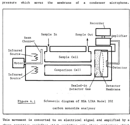
are continuous (rather than discrete) analysers and the dynamic

properties of these have been described by Larsen et a l . (1965),

Saltzman (1970) and Schnelle and Neeley (1972). It is important for

the time resolution of continuous analysers to satisfy the objectives

of the measurement program, and in particular to be dynamically fast

enough so that transient violations of air quality standards will be

detected. The dynamic properties of continuous analysers will be

considered in some detail in Chapter 4.

Most air pollution measurements are made at fixed locations. The

data obtained from such a fixed monitoring station can, in the

strictest sense, only be associated with that particular point.

However, it is common practice to assume that data from a fixed station

represent the air quality in a certain geographical area surrounding

the station. Whether this assumption is reasonable depends on a number

of factors such as the type of pollutant, the time period over which

the pollutant concentrations are averaged and the proximity of the

monitoring station to local pollution sources. In general this

assumption is more reasonable for longer averaging times such as one

month or one year. However, if pollutant concentrations averaged over

shorter periods (such as one day or one hour) are of interest then the

assumption may be invalid. Certainly the findings of Goldstein and

Landovitz (1977a, 1977b) seem to indicate that in New York City the

daily average measurements of sulphur dioxide and sraokeshade obtained

at 40 air monitoring stations do not adequately represent the areas

particularly difficult since Ott (1972) has shown that eight-hour

carbon monoxide concentrations can vary by a factor of three between

sites which are less than three kilometers apart. Some guidelines for

the selection of sites for carbon monoxide monitoring have been

provided by Ludwig and Kealoha (1975), although it is apparent that

there is no perfect station siting plan (Bryan, 1976). Generally it is

necessary to strike a balance between the density of the monitoring

network and the costs of operating the monitoring program. There have

been calls for development of procedures such as small and unobtrusive

individual air pollution monitors in order to obtain better estimates

of air pollutant exposure in urban populations (Morgan and Morris,

1977). Such devices may be able to provide data which supplement those

from the fixed monitoring stations.

Fully automated air quality monitoring systems which use

telecommunications to provide a direct link between the field

monitoring stations and the central office of the control agency have

been described by Zimmer (1976). These fully automated systems may

operate in delayed batch mode or real time mode. The delayed batch

mode is the more common, with data being measured and recorded at the

field station and transmitted to the central office only once or twice

a day. In the real time mode the data are transmitted from the field

station to the central office as the data are being recorded. The real

time mode permits real time modeling and instantaneously provides data

for management decision making, but the high costs of a real time

system do not justify its use in most situations.

Finally, it should be remembered that the data obtained from

fixed monitoring stations normally provide the basis for calibration or

validation of air pollution models. This fact should be recognised in

the siting of monitoring stations so that maximum use can be made of

the data they provide in air pollution modeling studies.

2.4 Urban Air Pollution Modeling

Air pollution modeling for entire urban areas is a relatively

recent development. The first such model was suggested for the Los

Angeles area by Frenkiel (1956). Since that time there has been a

dispersion of airborne pollutants over cities. The subject area of

urban air pollution modeling has been reviewed by several authors (for

example, Fan and Horie, 1971; Johnson, 1974; Pasquill, 1974; Hanna,

1975; Eschenroeder, 1975; Johnson et al., 1976; Turner, 1979; and

Johnson, 1979a) and no attempt is made here to provide a comprehensive

review of the subject. Rather, the various types of models are briefly

described while discussion of the modeling of dispersion of vehicular

pollutants from roadways will be deferred until Chapter 6. More

emphasis than usual is given to stochastic and time series models since

these have received relatively little attention in the reviews.

2.4.1 Mass Conservation Models

The mass conservation approach gives rise to two main types of

models, namely the Eulerian or multibox and the Lagrangian. In the

Eulerian models the atmosphere over a region is divided into boxes by

specifying a fixed horizontal grid and restricting attention to a layer

of air between the ground and an upper boundary, usually the inversion

base. The number of vertical divisions is usually kept fixed and

variation of the height of the inversion base is allowed for by

variation of the vertical dimension of the boxes. By contrast the

Lagrangian models are characterised by a framework which moves with the

air mass. However, wind shear causes distortion of the framework which

poses difficulties such as the accurate introduction of source

emissions to the system. This problem can be avoided by considering

the movement of only a single cell, models of which are known as

trajectory models.

The solution of both the Eulerian and Lagrangian formulations

presents problems. For example, the accurate treatment of the

advective terms is difficult in the Eulerian formulation, while in the

Lagrangian formulation the difficulty encountered in specification of

the turbulent diffusion term usually leads to it being ignored. The

concepts of advection and turbulent diffusion are described in more

detail later in this sub-section.

An alternative to either the Eulerian or Lagrangian formulations

is the particle-in-cell method which Sklarew et al. (1972) have

modified to include diffusive transport. This is essentially a hybrid

e a c h p a r t i c l e may be c o n s i d e r e d a s a L a g r a n g i a n c e l l moving i n r e l a t i o n t o a f i x e d E u l e r i a n framework.. The number of p a r t i c l e s i n e a c h E u l e r i a n c e l l a t any t i m e i s t h e n u s e d t o i n d i c a t e t h e mean c o n c e n t r a t i o n of p o l l u t a n t i n t h a t c e l l a t t h a t t i m e .

J o h n s o n e t a l . ( 1 9 7 6 ) have compared t h e c o m p u t a t i o n a l r e q u i r e m e n t s of E u l e r i a n , L a g r a n g i a n and p a r t i c l e - i n - c e l l m od el s and c o n c l u d e t h a t e a c h o f t h e t h r e e t y p e s h a s c o m p u t a t i o n a l a d v a n t a g e s f o r s p e c i f i c a p p l i c a t i o n s . Wh i le c o n s i d e r a t i o n o f t h e c o m p u t a t i o n a l r e q u i r e m e n t s i s i m p o r t a n t , i t s h o u l d n o t be t h e o n l y c r i t e r i o n u s e d f o r t h e s e l e c t i o n of a p a r t i c u l a r model s i n c e t h e d a t a r e q u i r e m e n t s o f m od el s may d i f f e r g r e a t l y and t h e d a t a p r e p a r a t i o n may p l a c e h e a v y demands on c o m p u t a t i o n t i m e ( J o h n s o n , 1 9 8 0 a ) . I n t h e f o l l o w i n g d e s c r i p t i o n of t h e mass c o n s e r v a t i o n a p p r o a c h t o a i r p o l l u t i o n m o d e l i n g a t t e n t i o n i s l i m i t e d t o t h e E u l e r i a n f o r m u l a t i o n . T h i s i s done b o t h f o r s i m p l i c i t y o f e x p o s i t i o n and t o i n t r o d u c e t h e t y p e o f model wh i ch i s e x am in ed i n C h a p t e r 7.

The m a t h e m a t i c a l f o r m u l a t i o n o f m od el s b a s e d upon t h e mass c o n s e r v a t i o n a p p r o a c h u s u a l l y b e g i n s w i t h t h e c o n t i n u i t y e q u a t i o n ( 2 . 1 ) , w h i c h d e s c r i b e s t h e b e h a v i o u r of N c h e m i c a l l y r e a c t i v e c o n s t i t u e n t s s u s p e n d e d i n a f l u i d

3c. 3 ( u c . ) 3 ( v c . ) 3 ( w c . )

1 + — + — — i —

3y

3 2i

v-

3 2c

3y2

3 2c

- ) + R. + S.

, 2 i i

(2. 1)

wher e c^ i s t h e i n s t a n t a n e o u s c o n c e n t r a t i o n o f t h e i t h c o n s t i t u e n t a t t h e p o i n t ( x , y , z ) and t i m e t i n a r e c t a n g u l a r c o - o r d i n a t e s y s t e m

u , v , w a r e t h e i n s t a n t a n e o u s v e l o c i t y c o mp o n en t s d e s c r i b i n g t h e m o t i o n of t h e f l u i d a t t h e p o i n t ( x , y , z ) a t t i m e t D-j_ i s t h e m o l e c u l a r d i f f u s i v i t y o f t h e i t h c o n s t i t u e n t