FPGA Implementation of Variable Feed Rate Algorithm for a Three Input Fuzzy Controller to Maintain the Cane Level

Abstract: Fuzzy logic which is one of methodology of soft computing has provided to be brilliant choice for the many control system application. Fuzzy logic is practical to numerous fields. One of the uses of fuzzy logic is in sugar mill. It is very important to produce sugar at low cost. Irregular supply of sugar cane decreases the efficiency of cane juice extraction during manufacturing of sugar. To increase the efficiency of cane juice extraction it is necessary to sustain the cane height at desired level inside Donnelly chute. A methodology to develop a variable feed rate algorithm for three inputs fuzzy controller sustains the cane height at desired level and was developed with fuzzy logic tool box of MATLAB software. The developed fuzzy controller can be implemented by using HDL language and Xilinx Vivado 2016.2.

Index Terms: fuzzy logic, fuzzy controller, HDL language

I. INTRODUCTION

Sugar producing from sugar cane happens in a specific period of year. India was second biggest maker of sugar on the planet after Brazil. It is a test to create sugar of good quality at lower cost which requires improvement in sugar making process. Over 60% of the globe sugar is generated as of sugar cane along with the parity is from sugar beet [1]. In India 60 million farmers depends on cane cultivation [2].

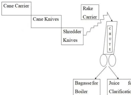
The flow of sugar making Process is described below. Cane billets were transformed into cane fiber during sugar making process. Cane billets are placed on cane carrier. The cane is passed through rotating knives, by which cane is cut into little fibers about 1-2 cm. Cane juice is obtained through crushing fiber [2, 3, 4]. A schematic for juice extraction of cane is given in Figure 1.Arrangement of a mill is given in Figure 2. Various important mill parameters such as mean diameter of roll, work opening [5] and contact angle [6] are useful for finding the required parameters.The length of the roll (Lr) is 183cm, width of the roll (Bc) is 43.5cm, optimum angle (α) is 610 and roll speed (S) is in (m/s). Escribed volume of cane (m3/s) is given by [7].

Ve = Lr × Bc × S Cosα (1) If qc is the bulk density of cane at entry plane (350Kg/m3) then the crushing rate or mass flow rate (Kg/s) is given by

Qc = qc × Ve (2)

The carrier speed (cm/s) [8] is given by

Revised Manuscript Received on August 05, 2019

V. Sai Sri Krishna, PG Scholar, GMR Institute of Technology, India Yogesh Misra, Professor, Department of ECE, GMRIT, India G. Anantha Rao, Sr. Assistant Professor, Department of ECE, GMRIT, Rajam, India.

Carrier Speed (cm/s) = (Feed Rate) / (Mass of cane in 1cm of

Carrier) (3)

The motor speed (rpm) [8] is given by

Motor Speed = (1.91 × Srake) rpm (4)

Where Srake = rake carrier speed cm/s

II. THREE INPUTS FUZZY CONTROLLER DESIGN AND VARIABLE FEED RATE ALGORITHM The three inputs fuzzy controller [9] to sustain cane height is given in Figure 3. Rake carrier prepared cane weight, Donnelly chute level of cane and the roll rotational speed are three variables used for extraction of cane juice. The Donnelly chute height, speed of rake carrier motor and the variation in prepared cane on the carrier are 180cm, 17rpm to 116rpm and 500Kg to 1000Kg respectively. The length, width and depth of chute are 180cm, 43.5cm and 183cm. The length, width and weight of rake carrier are 800cm, 150cm and 500kg. The endeavour of this algorithm depends on three variables values to vary rake carrier speed such that cane level in the Donnelly chute remains constant. The input parameters weight, height and roll speed are given in Figure 5, Figure 6 and Figure 7. The output parameter speed is given in Figure 8. Three inputs development algorithm [10] is given in Figure 4. The rules for roll speed for 12cm/s, 14.3cm/s, 16.6cm/s are given in Table I, Table II and Table III. The flow rate (Qc) when roll speed is 12.0cm/s , 14.3cm/s and 16.6cm/s from (2) is 19.3Kg/s, 22.8Kg/s and 26.6Kg/s.

The cane weight on rake carrier, cane level and roll rotational speed are the three inputs to fuzzy controller. Three sensors are required to sense the cane in the rake carrier, cane height in chute and rotational speed of rolls are load cell, light sensor tacho generator sensor. Amount of cane present on rake carrier is given by load cell. A load cell signal conditioning system [8] is explained. Level of cane in chute is determined by using height sensor. A signal conditioning system for height sensing [8] is explained.

Rotational speed of roll is measured using tacho generator. A signal conditioning system for tacho generator [8] is explained. The digital values obtained from analog digital converter by using the output of signal conditioning system for cane weight, cane level and roll speed are given in Figure 6, Figure 7 and Figure 8.

III. IMPLEMENTATION OF ALGORITHM OF FUZZY CONTROLLER USING VHDL

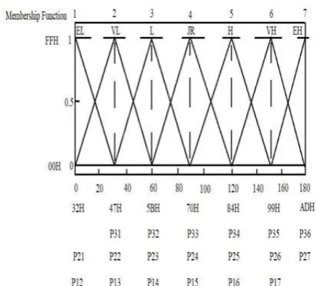
The fuzzification in terms of VHDL code is done as follows. Triangular membership function is given in Figure 9. It contains three points namely point-1, point-2 and point-3. The slopes of membership graph are represented by slope-1 and slope-2 and they are calculated from (5) and (6).

Slope-1 = (y2 – y1) ÷ (Point-2 – Point-1) (5) Slope-2 = (y2 – y1) ÷ (Point-3 – Point-2) (6) Where y2 is 1 (FFH) maximum value of a membership function and y1 is 0 (00H) minimum value of a membership function.The degree of membership of any value on x-axis less than or equal to the value of point-1 and greater than or equal to the value of point-3 is always 0. The degree of membership of any value on x-axis greater than the value of Point-1 and less than Point-2 is calculated from (7) and (8). µ = (Input Value – Point-1) × Slope-1 (7) The degree of membership of any value on x-axis greater than or equal to the value of Point-2 and less than Point-3 is calculated as follows:

µ = (Input Value – Point-2) × Slope-2 (8) The notations used in representing a point in a membership function are as follows:

P represents the point, 1st digit represents number of point (i.e. Point-1, Point-2 or Point-3) of membership function graph and 2nd digit represents the number of linguistic variable.

A. Fuzzification of Weight

The linguistic variables of weight are given in Figure 6. The digital values obtained from analog to digital converter by using signal conditioning system of cane weight are the values given to linguistic variables. For instance Point-3 of linguistic variable SL is represented by P31, Point-2 of linguistic variable UH is represented by P210 and Point-1 of linguistic variable SH is represented by P111. The x-axis represents variation of cane weight from 500Kg to1000Kg.

B. Slope Calculation of Weight

(i) Calculation of slopes of Linguistic Variable SL

Point-2 and Point-3 of SL is represented by P21 and P31 and its Slope-2SL is calculated from (6)

Slope-2SL = [(FFH – 00H) / (P31 – P21)] = [FFH / (1BH – 00H)] = 09H

(ii) Calculation of slopes of Linguistic Variable UL

(a)Point-1 and point-2 of UL is represented by P12 and P22 respectively and its Slope-1UL is calculated from (5)

Slope-1UL = [(FFH – 00H) / (P22 – P12)] = [FFH / (1BH – 00H)] = 09H

(b)Point-3 of UL is represented by P32 and its Slope-2UL is calculated from (6)

Slope 2UL = [(FFH – 00H) / (P32 – P22)] = [FFH / (34H – 1BH)] = 0AH (iii) Calculation of slopes of Linguistic Variable EL

(a)Point-1 and point-2 of EL is represented by P13 and P23 respectively and its Slope-1EL is calculated from (5)

Slope-1EL = [(FFH – 00H) / (P23 – P13)]

= [FFH / (34H – 1BH)] = 0AH

(b)Point-3 of EL is represented by P33 and its Slope-2EL is calculated from (6)

Slope 2EL = [(FFH – 00H) / (P33 – P23)] = [FFH / (4DH – 34H)] = 0AH

Similarly for all the Linguistic variables of input parameter WEIGHT slopes are calculated and are given in Table IV.

C. Fuzzification of Height

The linguistic variables of height are given in Figure 7. The digital values obtained from analog to digital converter by using signal conditioning system of cane level are the values given to linguistic variables. The x-axis represents variation of cane level from 0cm to 180cm.

D. Slope Calculation of Height

(i) Calculation of slopes of Linguistic Variable EL

Point-2 and Point-3 of EL is represented by P21 and P31 and its Slope-2EL is calculated from (6)

Slope-2EL = [(FFH – 00H) / (P31 – P21)] = [FFH / (47H – 32H)] = 0CH

(ii) Calculation of slopes of Linguistic Variable VL

(a)Point-1 and point-2 of VL is represented by P12 and P22 respectively and its Slope-1VL is calculated from (5)

Slope-1VL = [(FFH – 00H) / (P22 – P12)] = [FFH / (47H – 32H)] = 0CH

(b)Point-3 of VL is represented by P32 and its Slope-2VL is calculated from (6)

Slope 2VL = [(FFH – 00H) / (P32 – P22)] = [FFH / (5BH – 47H)] = 0CH

(iii) Calculation of slopes of Linguistic Variable L

(a)Point-1 and point-2 of L is represented by P13 and P23 respectively and its Slope-1L is calculated from (5)

Slope-1L = [(FFH – 00H) / (P23 – P13)] = [FFH / (5BH – 47H)] = 0CH

(b)Point-3 of L is represented by P33 and its Slope-2L is calculated from (6)

Slope 2L = [(FFH – 00H) / (P33 – P23)] = [FFH / (70H – 5BH)] = 0CH

Similarly for all the Linguistic variables of input parameter HEIGHT slopes are calculated and are given in Table V.

E. Fuzzification of Roll Speed

The linguistic variables of roll speed are given in

Figure 8. The digital values obtained from analog to digital converter by using signal conditioning system of roll speed are the values given to linguistic variables. The x-axis represents variation of roll speed from 12.0cm/s to 16.6cm/s.

F. Slope Calculation of Roll Speed

= [FFH / (E6H – D5H)] = 0FH

(b)Point-3 of RM is represented by P32 and its Slope-2RM is calculated from (6)

Slope 2RM = [(FFH – 00H) / (P32 – P22)] = [FFH / (F6H – E6H)] = 0FH

(iii) Calculation of slopes of Linguistic Variable RR

Point-1 and Point-2 of RR is represented by P13 and P23 and its Slope-1RR is calculated from (5)

Slope-1RR = [(FFH – 00H) / (P23 – P13)] = [FFH / (F6H – E6H)] = 0FH

Slopes for all the Linguistic variables of input parameter ROLL SPEED slopes are calculated and are given in Table VI.

Example-I:

Let the values of cane weight, cane height and roll speed at some instant is 720Kg, 80cm and 14.6cm/s.

G. Calculation of Degree of Membership of WEIGHT The load cell generates 16.26mV for 720Kg cane weight. The output of signal conditioning system of load cell for 16.26mV is 1.100V is given in Figure 10. The output of ADC when it receives 1.100V analog voltage is (0111 0000) and it is represented as 70H in hexadecimal. The 70H value will intersect linguistic variables L and JR of cane WEIGHT is given in Figure 6.

The degree of membership of this input value for linguistic variable L is calculated from (8)

µL = 1 – (Input Value – P25) × Slope-2L = FFH – (70H – 66H) × 09H

= A5H = 165D

The degree of membership of this input value for linguistic variable JR is calculated from (7)

µJR = (Input Value – P16) × Slope-1JR = (70 – 66H) × 09H

= 5AH = 90D

The degree of membership of 720Kg cane in nine linguistic variables is zero and it is given below for all eleven linguistic variables of input parameter WEIGHT.

µL = A5H, µJR = 5AH, and µSL = µUL = µEL = µVL = µH = µVH = µEH = µUH = µSH = 0

The simulation result showing the membership of linguistic variable L and JR when cane weight is 720Kg is given in Figure 11.

H. Calculation of Degree of membership of HEIGHT The height sensor will generate 14.7mA when cane is 80cm from the base of the Donnelly chute. Signal conditioning system for height sensing gives output of 1.469V for 14.7mA input is depicted in Figure 12. The output of ADC when it

variable JR is calculated from (7)

µJR = (Input Value – P14) × Slope-1JR = (69H – 5BH) × 0CH

= A8H = 168D

The degree of membership of 80cm cane from the base of Donnelly Chute in five linguistic variables is zero and it is given below for all seven linguistic variables of input parameter HEIGHT.

µL = 57H, µJR = A8H, µEL = µVL = µH = µVH = µEH = 0

The simulation result showing the membership of linguistic variable L and JR when cane height is 80cm is given in Figure 13.

I. Calculation of Degree of Membership of ROLL SPEED

Tacho generator gives output of 185µV for roll speed 14.6cm/s. Signal conditioning system for tacho generator gives output of 2177mV for 185µV is depicted in Figure 14. ADC gives analog voltage is (1110 1000) and E8H in hexadecimal for input 2177mV. The E8H value will intersect linguistic variables RM and RR of ROLL SPEED is given in Figure 8

The degree of membership of this input value for linguistic variable RM is calculated from (8)

µRM = 1 – (Input Value – P22) × Slope-1RM = FFH – (E8H – E6H) × 0FH

= E1H =225D

The degree of membership function of this input value for linguistic variable RR is calculated from (7)

µRR = (Input Value – P13) × Slope-1RR = (E8H – E6H) × 0FH

= 1EH = 30D

The degree of membership of roll speed 14.6cm/s in one linguistic variable is zero and it is given below for all three linguistic variables of input parameter ROLL SPEED.

µRL = 0, µRM = E1H, µRR = 1EH

The simulation result showing the membership of linguistic variable RL, RM and RR

when roll speed is 14.6cm/s is depicted in Figure 15.

J. Implementation of Rule Inference Algorithm

In continuation with Example-I, the cane weight of 720Kg has degree of membership in L and JR linguistic variables of input parameter WEIGHT, the cane height of 80cm has degree of membership in L and JR linguistic variables in input parameter HEIGHT and the roll speed 14.6cm/s has degree of membership in RM and RR linguistic variables in input parameter ROLL SPEED. Total 186 rules having L and JR linguistic variables in both

The fired rules are represented in Table I, Table II and Table III in bold and italic manner.The part of VHDL code for finding minimum degree of membership value of each rule is given in Figure 16. The minimum degree of membership among the three antecedents of all fired rules is

MinR (103) = 57H, MinR (104) = 57H, MinR (114) = A5H, MinR (115) = 5AH, MinR (180) = 1EH, MinR (181) = 1EH, MinR (191) = 1EH, MinR (192) = 1EH and minimum value of all remaining fired rules is 00H. The minimum degree of membership value results are given in Figure 17 and Figure 18.

The maximum value of consequents among all the fired rules having same output linguistic variable is chosen as the final fuzzy value of corresponding linguistic variable. The final value of EL is represented by MaxR (0), VL by MaxR (1), L by MaxR (2), JR by MaxR (3), H by MaxR (4), VH by MaxR (5), EH by MaxR (6), UH by MaxR(7) and SH by MaxR (8). The part of VHDL code for finding the maximum value of all rules having same consequent is given in Figure 19. The maximum value of consequents among all the fired rules of Example-I are

MaxR (0) = 00H, MaxR (1) = 00H, MaxR (2) = 5AH, MaxR (3) = A5H, MaxR (4) = 1EH, MaxR (5) = 00H, MaxR (6) = 00H, MaxR (7) = 00H, MaxR (8) = 00H. The maximum values of consequents obtained are shown in Figure 20.

K. Implementation of Defuzzification Algorithm

Defuzzification changes fuzzy output into crisp output. The Sugeno style of fuzzy logic is used as it requires only singleton value. The singleton values of all linguistic variables of output parameter SPEED (Figure 9) are given below.

Singleton value of linguistic variable EL = SEL = 17H Singleton value of linguistic variable VL = SVL = 1DH Singleton value of linguistic variable L = SL = 2AH Singleton value of linguistic variable JR = SJR= 36H Singleton value of linguistic variable H = SH = 43H Singleton value of linguistic variable VH = SVH = 4FH Singleton value of linguistic variable EH = SEH = 5CH Singleton value of linguistic variable UH = SUH = 68H Singleton value of linguistic variable SH = SSH = 6EH The crisp (defuzzified) output is obtained from (9)

Crisp Output = (Numerator) / (Denominator) (9) Here,

Numerator = [{MaxR (0) × SEL} + {MaxR (1) × SVL} + {MaxR (2) × SL} + {MaxR (3) × SJR} + {MaxR (4) × SH} + {MaxR (5) × SVH} + {MaxR (6) × SEH} + {MaxR (7) ×

SUH} + {MaxR (8) × SSH}] (10) Denominator = MaxR (0) + MaxR (1) + MaxR (2) + MaxR

(3) + MaxR (4) + MaxR (5) + MaxR (6) + MaxR (7) + MaxR (8) (11) From Example-I results are obtained as Numerator = 396CH (0011100101101100) is obtained from (10) and Denominator = 011DH (0000000100011101) is obtained from (11) and Crisp output = 33H = 51D (rpm) is obtained from (9). The crisp output result is depicted in Figure 21.

IV. RESULTS AND DISCUSSION

Three inputs fuzzy controller developed using algorithm is implemented using VHDL by using Xilinx Vivado 2016.2

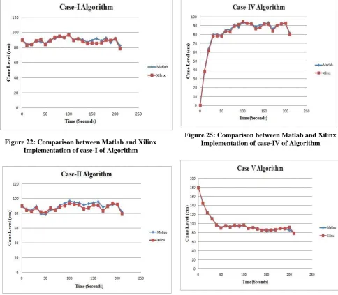
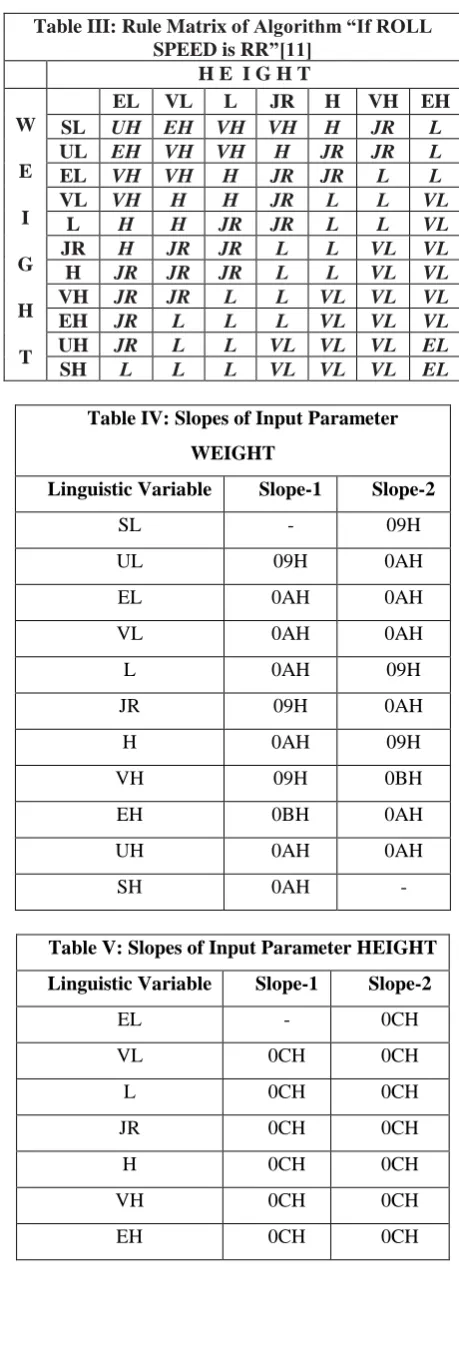
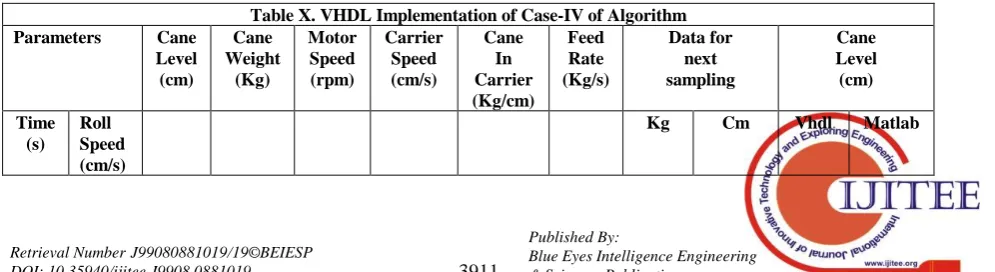
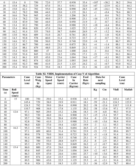
software. Cane weight, cane level and the roll speed during each sampling is kept same as the corresponding cases of Algorithm of MATLAB design [10]. The results obtained for algorithm using VHDL by using Xilinx Vivado are compared with Algorithm of MATLAB design.In case-I and case-II the cane weight and cane level values for the first simulation are 750Kg and 90cm correspondingly. In case-I, case-III and case-V roll speed for the first simulation is 15cm/s. In case-II, case-IV and case-VI roll speed for the first simulation is 15.4cm/s. The cane level values obtained by using Xilinx Vivado compared with Matlab for case-I and case-II is depicted in Table VII and Table VIII. In case-III and case-IV the cane weight and cane level for the first simulation are 750Kg and 0cm correspondingly. The cane level values obtained by using Xilinx Vivado compared with Matlab for case-III and case-IV is given by Table IX and Table X. In Case-V and Case-VI the cane weight and cane level for the first simulation are 750Kg and 180cm correspondingly. The cane level values obtained by using Xilinx Vivado compared with Matlab for case-V and case-VI is given by Table XI and Table XII. Comparison between Matlab and Xilinx results of case-I is depicted in Figure 22 and Table XIII. Comparison between Matlab and Xilinx results of case-II is given in Figure 23 and Table XIV. Comparison between Matlab and Xilinx results of case-III is depicted in Figure 24 and Table XV. Comparison between Matlab and Xilinx results of case-IV is given in Figure 25 and Table XVI. Comparison between Matlab and Xilinx results of case-V is given in Figure 26 and Table XVII. Comparison between Matlab and Xilinx results of case-VI are given in Figure 27 and Table XVIII. Comparison between all six cases of Matlab and Xilinx results is given in Figure 28 and Table XIX.

V. CONCLUSION

The fuzzy controller maintains cane level in the range 85cm to 95cm for an average 69.75% of simulation duration. Time required for reaching cane level at 90cm for case-III, case-IV, case-V and case-VI are 57.8 seconds, 79.4 seconds, 109.5 seconds and 49.2 seconds respectively. Lowest level of cane in chute for case-I, case-II, case-V and case-VI are 78.7cm, 79.1cm, 78.7cm and 80.5cm respectively. Highest level of cane in chute for case-I, case-II, case-III and case-IV are 97. 1cm, 93.9cm, 97.6cm and 94.6cm respectively. Percentage of time cane level is in between 85cm to 95cm for case-I, case-II, case-III, case-IV, case-V and case-VI are 84.8%, 76.2%, 60.0%, 62.2%, 62.7% and 72.6% respectively.

ACKNOWLEDGEMENT

Figure 1: Schematic of Cane Juice Extraction Process

Figure 2: Two Rolls and Chute Arrangement of a Mill

Figure 3: Three Inputs Fuzzy Controller to Maintain Cane Level

Figure 5: Fuzzified Input Parameter WEIGHT with Point Representation

Figure 6: Fuzzified Input Parameter HEIGHT with Point Representation

Figure 7: Fuzzified Input Parameter ROLL SPEED with Point Representation

Figure 8: Output Parameter SPEED

Figure 9: Triangular Membership Function

Figure 11: Degree of Membership when Cane Weight is

Figure 12: Output of Cane Level Sensing Signal Conditioning when Cane is at 80cm in Chute

Figure 13: Degree of membership when Cane Height is 80cm µL = dmf_h_f[1] = 57H, µJR = dmf_h_f[2] = A8H

Figure 14: Output of Roll Speed Signal Conditioning System when its Speed is 14.6cm/s

Figure 15: Degree of membership when Roll Speed is 14.6 cm/s µRL = dmf_r_f[0] = 00H, µRM = dmf_r_f[1] = E1H,

µRR = dmf_r_f[2] = 1EH PROCESS (DMF_R_F, DMF_H_F, DMF_W_F) BEGIN

minR(0) <= min(DMF_R_F(0), DMF_H_F(0), DMF_W_F(0);

minR(1) <= min(DMF_R_F(0), DMF_H_F(0), DMF_W_F(1);

minR(2) <= min(DMF_R_F(0), DMF_H_F(0), DMF_W_F(2);

minR(3) <= min(DMF_R_F(0), DMF_H_F(0), DMF_W_F(3);

Figure 17: VHDL Simulation Showing MinR (103), MinR (104), MinR (114) and MinR (115)

Figure 18: VHDL Simulation Showing MinR (180), MinR (181), MinR (191), MinR (192)

MaxR(5) <= max5(minR(79), minR(80), minR(89),

minR(90), minR(99), minR(100), minR(110), minR(158), minR(159), minR(168), minR(169), minR(178), minR(188)); MaxR(6) <= max6(minR(78), minR(88), minR(156), minR(157), minR(166), minR(167), minR(176), minR(177), minR(187));

MaxR(7) <= max7 (minR(77), minR(155), minR(165)); MaxR(8) <= max8 (minR(154));

Figure 19: Part of VHDL code for finding the maximum value of all rules having same consequent

Figure 20: VHDL Simulation Showing the values of Linguistic Variables of Output Parameter SPEED

Figure 22: Comparison between Matlab and Xilinx Implementation of case-I of Algorithm

Figure 23: Comparison between Matlab and Xilinx Implementation of case-II of Algorithm

Figure 24: Comparison between Matlab and Xilinx Implementation of case-III of Algorithm

Figure 25: Comparison between Matlab and Xilinx Implementation of case-IV of Algorithm

Figure 26: Comparison between Matlab and Xilinx Implementation of case-V of Algorithm

Figure 28: Comparison between all six cases of Matlab and Xilinx Implementation of Algorithm

Table I: Rule Matrix of Algorithm “If ROLL SPEED is RL”[11]

H E I G H T

W

E

I

G

H

T

EL VL L JR H VH EH

SL VH VH H H JR L L

UL VH H H JR L L L

EL H H JR JR L L VL

VL H JR JR L L VL VL

L JR JR JR L L VL VL

JR JR JR L L VL VL VL

H JR L L L VL VL EL

VH L L L VL VL VL EL

EH L L L VL VL VL EL

UH L L VL VL VL EL EL

SH L VL VL VL VL EL EL

Table II: Rule Matrix of Algorithm “If ROLL SPEED is RM”[11]

H E I G H T

W

E

I

G

H

T

EL VL L JR H VH EH

SL UH EH VH VH H JR L

UL EH VH VH H JR JR L

EL VH VH H JR JR L L

VL VH H H JR L L VL

L H H JR JR L L VL

JR H JR JR L L VL VL

H JR JR JR L L VL VL

VH JR JR L L VL VL VL

EH JR L L L VL VL VL

UH JR L L VL VL VL EL

SH L L L VL VL VL EL

Table III: Rule Matrix of Algorithm “If ROLL SPEED is RR”[11]

H E I G H T

W

E

I

G

H

T

EL VL L JR H VH EH

SL UH EH VH VH H JR L

UL EH VH VH H JR JR L

EL VH VH H JR JR L L

VL VH H H JR L L VL

L H H JR JR L L VL

JR H JR JR L L VL VL

H JR JR JR L L VL VL

VH JR JR L L VL VL VL

EH JR L L L VL VL VL

UH JR L L VL VL VL EL

SH L L L VL VL VL EL

Table IV: Slopes of Input Parameter WEIGHT

Linguistic Variable Slope-1 Slope-2

SL - 09H

UL 09H 0AH

EL 0AH 0AH

VL 0AH 0AH

L 0AH 09H

JR 09H 0AH

H 0AH 09H

VH 09H 0BH

EH 0BH 0AH

UH 0AH 0AH

SH 0AH -

Table V: Slopes of Input Parameter HEIGHT Linguistic Variable Slope-1 Slope-2

EL - 0CH

VL 0CH 0CH

L 0CH 0CH

JR 0CH 0CH

H 0CH 0CH

VH 0CH 0CH

Table VII. VHDL Implementation of Case-I of Algorithm Parameters Cane

Level (cm)

Cane Weight

(Kg)

Motor Speed (rpm)

Carrier Speed (cm/s)

Cane In Carrier (Kg/cm)

Feed Rate (Kg/s)

Data for next sampling

Cane Level (cm) Time

(s)

Roll Speed (cm/s)

Kg Cm Vhdl Matlab

0 15 90 750 45.0 23.6 0.938 22.1 -19 -6.8 83.2 84.6

10 83.2 729 51.0 26.7 0.911 24.3 +3 +1.1 84.3 84.2

20 84.3 792 49.0 25.7 0.990 25.4 +14 +5.0 89.3 88.8

30 89.3 908 41.0 21.5 1.135 24.4 +4 +1.4 90.7 87.4

40 12.6 90.7 965 29.0 15.2 1.206 18.3 -19 -6.8 83.9 85.3

50 83.9 720 46.0 24.1 0.900 21.7 +15 +5.4 89.3 90.3

60 89.3 760 43.0 22.5 0.950 21.4 +12 +4.3 93.6 92.1

70 93.6 790 40.0 20.9 0.988 20.6 +4 +1.4 95.0 94.6

80 95.0 820 37.0 19.4 1.025 19.9 -3 -1.1 93.9 92.8

90 16.2 93.9 555 74.0 38.7 0.694 26.9 +9 +3.2 97.1 97.1

100 97.1 609 60.0 31.4 0.761 23.9 -21 -7.5 89.6 90.2

110 89.6 578 70.0 36.6 0.723 26.5 +5 +1.8 91.4 92.3

120 91.4 598 64.0 33.5 0.748 25.1 -9 -3.2 88.2 90.5

130 88.2 700 55.0 28.8 0.875 25.2 -8 -2.9 85.3 86.9

140 85.3 679 59.0 30.9 0.849 26.2 +2 +0.7 86.0 89.8

150 15.4 86.0 800 47.0 24.6 1.000 24.6 -1 -0.4 85.6 91.9

160 85.6 845 45.0 23.6 1.056 24.9 +2 +0.7 86.3 89.0

170 86.3 835 47.0 24.6 1.044 25.7 +10 +3.6 89.9 92.9

180 89.9 874 43.0 22.5 1.093 24.6 -1 -0.4 89.5 86.8

190 89.5 900 43.0 22.5 1.125 25.3 +6 +2.1 91.6 92.2

200 91.6 924 35.0 18.3 1.155 21.1 -36 -12.9 78.7 82.6

Table VIII. VHDL Implementation of Case-II of Algorithm Parameters Cane

Level (cm)

Cane Weight

(Kg)

Motor Speed (rpm)

Carrier Speed (cm/s)

Cane In Carrier

Feed Rate (Kg/s)

Data for next sampling

Time (s)

Roll Speed (cm/s)

Kg Cm Vhdl Matlab

0 15.4 90 750 47 24.6 0.938 23.1 -16 -5.7 84.3 85.7

10 15.8 84.3 729 52.0 27.2 0.911 24.8 -5 -1.8 82.5 84.3

20 15.0 82.5 792 49.0 25.7 0.990 25.4 +14 +5.0 87.5 89.7

30 16.2 87.5 908 41.0 21.5 1.135 24.4 -16 -5.7 81.8 79.0

40 16.6 81.8 965 42.0 22.0 1.206 26.5 -1 -0.4 81.4 78.6

50 13.4 81.4 720 49.0 25.7 0.900 23.1 +16 +5.7 87.1 84.7

60 13.8 87.1 760 43.0 22.5 0.950 21.4 -7 -2.5 84.6 85.1

70 13.4 84.6 790 44.0 23.0 0.988 22.7 +12 +4.3 88.9 91.2

80 15.4 88.9 820 47.0 24.6 1.025 25.2 +5 +1.8 90.7 93.7

90 16.2 90.7 555 74.0 38.7 0.694 26.9 +9 +3.2 93.9 96.9

100 13.0 93.9 609 51.0 26.7 0.761 20.3 -5 -1.8 92.1 94.8

110 14.3 92.1 578 60.0 31.4 0.723 22.7 -2 -0.7 91.4 94.4

120 14.6 91.4 598 56.0 29.3 0.748 21.9 -15 -5.4 86.0 91.5

130 12.3 86.0 700 44.0 23.0 0.875 20.1 +4 +1.4 87.4 93.3

140 12.6 87.4 679 48.0 25.1 0.849 21.3 +11 +3.9 91.3 94.4

150 15.4 91.3 800 47.0 24.6 1.000 24.6 -1 -0.4 90.9 95.8

160 12.0 90.9 845 31.0 16.2 1.056 17.1 -21 -7.5 83.4 88.7

170 14.3 83.4 835 45.0 23.6 1.044 24.6 +17 +6.1 89.5 90.5

180 14.6 89.5 874 43.0 22.5 1.093 24.6 +12 +4.3 93.8 91.9

190 15.0 93.8 900 40.0 20.9 1.125 23.5 -5 -1.8 92.0 92.3

200 15.4 92.0 924 35.0 18.3 1.155 21.1 -36 -12.9 79.1 81.9

Table IX. VHDL Implementation of Case-III of Algorithm Parameters Cane

Level (cm) Cane Weight (Kg) Motor Speed (rpm) Carrier Speed (cm/s) Cane In Carrier (Kg/cm) Feed Rate (Kg/s) Data for next sampling Cane Level (cm) Time (s) Roll Speed (cm/s)

Kg Cm Vhdl Matlab

0 15 0 750 70.0 36.6 0.938 34.3 +103 +36.8 36.8 35.4

10 36.8 729 64.0 33.5 0.911 30.5 +65 +23.2 60.0 59.7

20 60.0 792 56.0 29.3 0.990 29.0 +50 +17.9 77.9 79.7

30 77.9 908 44.0 23.0 1.135 26.1 +21 +7.5 85.4 86.8

40 12.6 85.4 965 32.0 16.8 1.206 20.3 +1 +0.4 85.8 85.4

50 85.8 720 46.0 24.1 0.900 21.7 +15 +5.4 91.2 90.8

60 91.2 760 42.0 22.0 0.950 20.9 +7 +2.5 93.7 92.2

70 93.7 790 40.0 21.0 0.988 20.7 +5 +1.8 95.5 95.1

80 95.5 820 37.0 19.4 1.025 19.9 -3 -1.1 94.4 93.7

90 16.2 94.4 555 74.0 38.7 0.694 26.9 +9 +3.2 97.6 96.9

100 97.6 609 60.0 31.4 0.761 23.9 -21 -7.5 90.1 89.8

110 90.1 578 70.0 36.6 0.723 26.5 +5 +1.8 91.9 91.6

120 91.9 598 64.0 33.5 0.748 25.1 -9 -3.2 88.7 89.5

130 88.7 700 54.0 28.3 0.875 24.8 -12 -4.3 84.4 86.3

140 84.4 679 59.0 30.9 0.849 26.2 +2 +0.7 85.1 83.8

150 15.4 85.1 800 47.0 24.6 1.000 24.6 -1 -0.4 84.7 85.2

160 84.7 845 45.0 23.6 1.056 24.9 +2 +0.7 85.4 85.9

170 85.4 835 47.0 24.6 1.044 25.7 +10 +3.6 89.0 89.1

180 89.0 874 43.0 22.5 1.093 24.6 -1 -0.4 88.6 88.4

190 88.6 900 44.0 23.0 1.125 25.9 +12 +4.3 92.9 90.9

200 92.9 924 35.0 18.3 1.155 21.1 -36 -12.9 80.0 80.2

Table X. VHDL Implementation of Case-IV of Algorithm Parameters Cane

Level (cm) Cane Weight (Kg) Motor Speed (rpm) Carrier Speed (cm/s) Cane In Carrier (Kg/cm) Feed Rate (Kg/s) Data for next sampling Cane Level (cm) Time (s) Roll Speed (cm/s)

110 14.3 92.8 578 60.0 31.4 0.723 22.7 -2 -0.7 92.1 92.1

120 14.6 92.1 598 56.0 29.3 0.748 22.0 -14 -5 86.7 89.2

130 12.3 86.7 700 44.0 23.0 0.875 20.1 +4 +1.4 88.1 91.0

140 12.6 88.1 679 48.0 25.1 0.849 21.3 +11 +3.9 92.0 92.1

150 15.4 92.0 800 47 24.6 1.000 24.6 -1 -0.4 91.6 93.5

160 12.0 91.6 845 31.0 16.2 1.056 17.1 -21 -7.5 84.1 86.4

170 14.3 84.1 835 45.0 23.6 1.044 24.6 +17 +6.1 90.2 90.7

180 14.6 90.2 874 42.0 22.0 1.093 24.0 +6 +2.1 92.3 91.8

190 15.0 92.3 900 41.0 21.5 1.125 24.2 +2 +0.7 93.0 92.2

200 15.4 93.0 924 35.0 18.3 1.155 21.1 -36 -12.9 80.1 81.5

Table XI. VHDL Implementation of Case-V of Algorithm Parameters Cane

Level (cm)

Cane Weig

ht (Kg)

Motor Speed (rpm)

Carrier Speed (cm/s)

Cane In Carrier (Kg/cm)

Feed Rate (Kg/s)

Data for next sampling

Cane Level (cm) Time

(s) Roll Speed (cm/s)

Kg Cm Vhdl Matlab

0 15 180 750 29.0 15.2 0.938 14.3 -97 -34.6 145.4 145.7

10 145.4 729 38.0 19.9 0.911 18.1 -59 -21.1 124.3 123.9

20 124.3 792 39.0 20.4 0.990 20.2 -38 -13.6 110.7 111.8

30 110.7 908 34.0 17.8 1.135 20.2 -38 -13.6 97.1 97.5

40 12.6 97.1 965 29.0 15.2 1.206 18.3 -19 -6.8 90.3 91.8

50 90.3 720 46.0 24.1 0.900 21.7 +15 +5.4 95.7 95.4

60 95.7 760 39.0 20.4 0.950 19.4 -8 -2.9 92.8 92.9

70 92.8 790 41.0 21.5 0.988 21.2 +10 +3.6 96.4 95.0

80 96.4 820 37.0 19.4 1.025 19.9 -3 -1.1 95.3 93.6

90 16.2 95.3 555 73.0 38.2 0.694 26.5 +5 +1.8 97.1 96.8

100 97.1 609 60.0 31.4 0.761 23.9 -21 -7.5 89.6 89.7

110 89.6 578 70.0 36.6 0.723 26.5 +5 +1.8 91.4 91.5

120 91.4 598 64.0 33.5 0.748 25.1 -9 -3.2 88.2 89.4

130 88.2 700 55.0 28.8 0.875 25.2 -8 -2.9 85.3 86.2

140 85.3 679 59.0 26.2 0.849 26.2 +2 +0.7 86.0 83.7

150 15.4 86.0 800 47.0 24.6 1.000 24.6 -1 -0.4 85.6 85.1

160 85.6 845 45.0 23.6 1.056 24.9 +2 +0.7 86.3 85.8

170 86.3 835 47.0 24.6 1.044 25.7 +10 +3.6 89.9 89.0

180 89.9 874 43.0 22.5 1.093 24.6 -1 -0.4 89.5 88.3

190 89.5 900 43.0 22.5 1.125 25.3 +6 +2.1 91.6 85.8

200 91.6 924 35.0 18.3 1.155 21.1 -36 -12.9 78.7 80.4

Table XII. VHDL Implementation of Case-VI of Algorithm Parameters Cane

Level (cm)

Cane Weig

ht (Kg)

Motor Speed (rpm)

Carrier Speed (cm/s)

Cane In Carrier (Kg/cm)

Feed Rate (Kg/s)

Data for next sampling

Cane Level (cm) Time

(s) Roll Speed (cm/s)

Kg Cm Vhdl Matlab

10 15.8 142.9 729 41.0 21.5 0.911 19.6 -57 -20.4 122.5 122.1

20 15.0 122.5 792 40.0 20.9 0.990 20.7 -33 -11.8 110.7 111.7

30 16.2 110.7 908 38.0 19.9 1.135 22.6 -34 -12.1 98.6 102.1

40 16.6 98.6 965 38.0 19.9 1.206 24.0 -26 -9.3 89.3 90.0

50 13.4 89.3 720 49.0 25.7 0.900 23.1 +16 +5.7 95.0 96.1

60 13.8 95.0 760 40.0 20.9 0.950 19.9 -22 -7.9 87.1 86.5

70 13.4 87.1 790 44.0 23.0 0.988 22.7 +12 +4.3 91.4 91.1

80 15.4 91.4 820 47.0 24.6 1.025 25.2 +5 +1.8 93.2 93.6

90 16.2 93.2 555 74.0 38.7 0.694 26.9 +9 +3.2 96.4 95.7

100 13.0 96.4 609 50.0 26.2 0.761 19.9 -9 -3.2 93.2 94.3

110 14.3 93.2 578 60.0 31.4 0.723 22.7 -2 -0.7 92.5 93.9

120 14.6 92.5 598 56.0 29.3 0.748 21.9 -15 -5.4 87.1 91.0

130 12.3 87.1 700 44.0 23.0 0.875 20.1 +4 +1.4 88.5 92.8

140 12.6 88.5 679 48.0 25.1 0.849 21.3 +11 +3.9 92.4 90.7

150 15.4 92.4 800 47.0 24.6 1.000 24.6 -1 -0.4 92.0 88.6

160 12.0 92.0 845 31.0 16.2 1.056 17.1 -21 -7.5 84.5 87.9

170 14.3 84.5 835 45.0 23.6 1.044 24.6 +17 +6.1 90.6 90.8

180 14.6 90.6 874 42.0 22.0 1.093 24.0 +6 +2.1 92.7 91.9

190 15.0 92.7 900 41.0 21.5 1.125 24.2 +2 +0.7 93.4 92.3

200 15.4 93.4 924 35.0 18.3 1.155 21.1 -36 -12.9 80.5 91.2

Table XIII: Comparison between MATLAB and XILINX Implementation of Case-I of Algorithm

Parameter Matlab

Implement -ation of Algorithm Xilinx Implement -ation of Algorithm Percentage of time cane level is

in between 85 cm to 95 cm

89.1% 84.8%

Lowest Level of Cane in the Chute (cm)

82.6 78.7

Highest Level of Cane in the Chute (cm)

97.1 97.1

Slowest Speed of Carrier Motor (rpm)

31.1 29.0

Fastest Speed of Carrier Motor (rpm)

74.6 74.0

Slowest Speed of Cane Carrier (cm/s)

16.3 15.2

Fastest Speed of Cane Carrier (cm/s)

39.1 38.7

Mean Cane Level (cm) 89.6 88.7

Standard Deviation (cm) 3.5 4.2

Table XIV: Comparison between MATLAB and XILINX Implementation of Case-II of Algorithm

Parameter Matlab

Implement -ation of Algorithm Xilinx Implement -ation of Algorithm Percentage of time cane level is

in between 85 cm to 95 cm

69.5% 76.2%

Lowest Level of Cane in the 78.6 79.1

Chute (cm)

Highest Level of Cane in the Chute (cm)

96.9 93.9

Slowest Speed of Carrier Motor (rpm)

31.2 31.0

Fastest Speed of Carrier Motor (rpm)

74.1 74.0

Slowest Speed of Cane Carrier (cm/s)

16.3 16.2

Fastest Speed of Cane Carrier (cm/s)

38.8 38.7

Mean Cane Level (cm) 89.4 87.7

Standard Deviation (cm) 5.2 4.2

Table XV: Comparison between MATLAB and XILINX Implementation of Case-III of Algorithm

Parameter Matlab

Implement -ation of Algorithm Xilinx Implement -ation of Algorithm Percentage of time cane level is

in between 85 cm to 95 cm

69.1% 60.0%

Time required to reach cane level at 90 cm (sec)

58.5 57.8

Highest Level of Cane in the Chute (cm)

96.9 97.6

Slowest Speed of Carrier Motor (rpm)

31.4 32.0

Fastest Speed of Carrier Motor (rpm)

74.1 74.0

Slowest Speed of Cane Carrier (cm/s)

in between 85 cm to 95 cm Time required to reach cane level at 90 cm (sec)

78.1 79.4

Highest Level of Cane in the Chute (cm)

93.6 94.6

Slowest Speed of Carrier Motor (rpm)

31.2 31.0

Fastest Speed of Carrier Motor (rpm)

75.4 74.0

Slowest Speed of Cane Carrier (cm/s)

16.3 16.2

Fastest Speed of Cane Carrier (cm/s)

39.5 38.7

Table XVII: Comparison between MATLAB and XILINX Implementation of Case-V of Algorithm

Parameter Matlab

Implement -ation of Algorithm

Xilinx Implement

-ation of Algorithm Percentage of time cane level is

in between 85 cm to 95 cm

62.7% 62.7%

Time required to reach cane level at 90 cm (sec)

109.6 109.5

Lowest Level of Cane in the Chute (cm)

80.4 78.7

Slowest Speed of Carrier Motor (rpm)

29.5 29.0

Fastest Speed of Carrier Motor (rpm)

74.2 73.0

Slowest Speed of Cane Carrier (cm/s)

15.4 15.2

Fastest Speed of Cane Carrier (cm/s)

38.8 38.2

Table XVIII: Comparison between MATLAB and XILINX Implementation of Case-VI of Algorithm

Parameter Matlab Xilinx

(rpm)

Fastest Speed of Carrier Motor (rpm)

74.2 74.0

Slowest Speed of Cane Carrier (cm/s)

15.4 15.2

Fastest Speed of Cane Carrier (cm/s)

38.4 38.7

Table XIX: Comparison between all six cases of MATLAB and XILINX Implementation of Algorithm

Percentage of time cane level is in between 85 cm to 95 cm

Case-I Case-II Case-III Case-IV Case-V Case-VI

MATLAB Implementation of Algorithm 89.1% 69.5% 69.1% 70.2% 62.7% 72.8%

1. D.P Kulkarni, Cane Sugar Manufacture, The Sugar technologists association of India, New Delhi, 2002-03.

2. A jha, “India’s sugar policy and world sugar economy” in proc. FAO International sugar conference, Fiji, August 2012.

3. Indian Sugar Mills Association (ISMA), 2010, “Important Events” (online) at: http://www.indiansugar.com/EventDetails.

4. S. Ahmed, Indian Sugar Industry, Centre for management studies, Jamia Millia Islamia, New Delhi, India, Unpublished.

5. Kent, Geoffrey A, “Increasing the capacity of Australian raw sugar factory milling units”, PhD. Dissertation, school of Engineering, Mechanical Engineering Department, James Cook University, Brisbane, 2003. 6. Seturaman, P, “Design of an experimental apparatus to analyze bagasse behaviour in a chute”, M.E Dissertation, Queensland University of Technology, Brisbane, 2012.

7. Murry, C.R, Holt, J. E and Munro, B.M “An investigation of factory feed chutes” proc. Qd. Soc. Sug. Cane Tech. 29th conf., pp. 143, 1962. 8. Yogesh Misra, H R Kamath, “Implementation and Performance Analysis of a Three Inputs Conventional Controller to Maintain the Cane Level During Cane Crushing in FPGA using VHDL” International Journal of Engineering Research & Technology (IJERT) Vol.3, Issue9, September 2014.

9. Yogesh Misra, H R Kamath, “Analysis and Design of a Three Inputs Fuzzy System for Maintaining the Cane Level during Sugar

Manufacturing” journal of Automation and Control, 2014, Vol.2, No.3, pp.62-78.

10. Yogesh Misra, H R Kamath, “Development of Variable Feed Rate Algorithm for Three Inputs Fuzzy System to Maintain the Cane Level during Sugar Juice Extraction” Cooperative Sugar Journal, Vol.48, No.7, March 2015.

AUTHORS PROFILE

V. Sai Sri Krishna received his B.Tech degree in Electronics and Communication Engineering from Sri Vasavi Engineering College which is affiliated under JNTUK, Andhra Pradesh, India in 2017. He is pursuing his M.Tech degree in VLSI and Embedded Systems Design specialization in GMRIT which is affiliated under JNTUK, Andhra Pradesh, India. His areas of interest are ASIC design implementations and low power digital VLSI design.

Dr. Yogesh Misra has 24 years of industrial and teaching experience and currently working as Professor in Electronics and Communication Engineering Department of GMR Institute of Technology, Rajam, Andhra Pradesh, India. Dr. Misra has worked in U V Instruments (P) Ltd, a sugar mill automation company for many years. He has authored two books and his research interest includes VLSI and Embedded Computing. Dr. Misra is life member of ISTE.