Digital Image Edge Detection Using Cellular Automata

ISSN: 2278-3075, Volume-8 Issue-7S2, May 2019

Abstract: Cellular automata is a regular rid of cell and it’s a system which is dynamic in which space and time are discrete. This system consists of 1- dimensional, 2- dimensional, 3- dimensional and so on up to n-dimensional grid of cells. Every transaction state has pre define finite possible states according their transaction function. Any digital image also consider regular grid of cells called pixels, in given paper cellular automata is performed for image processing for the edge detection in digital image. Edges are insensibly variation in pixels intensity values it’s important for objects boundary detection and feature extraction of the image. This paper consider only binary image for the detection of edges and apply objective function for the selection of rule set from the Look up Table.

Keywords: Cellular Automata, Image denoising, Image Processing, Rule Selection.

I.INTRODUCTION

The easiest illustration of a Cellular Automata is a 1- dimensional array (two ways infinite possibily) of cells. Discrete is used to classify Time, every cell is at one of a finite set of feasible states at every point of time. At each clock pulse (cycle) the cells modifies its state, the current state of the cell and its RIGHT and LEFT neighbors fully determine new state. The function (known as local rule) which discovers this modification of state is the equivalent for every existing cells. The global or layout state of the Cellular Automata is termed as collection of cell states at any point of time is, and ascertain the stage of evolution of the Cellular Automata. At point of time t=0, the Cellular Automata is in some starting layout, and subsequently begin categorically under the consequence of the confined rule, that is pertain to every cell at each clock pulse. A (bi-directional, deterministic) CA is a triple A = (P; Q; δ), where P is a on-empty state set, Q is the neighborhood system, and δ: PQ→P is the local transition function (rule). This function explain the rules of evaluating the cell’s state at (t +1) time step, given the states of the closest cells at time step t.

If we talk of neighborhoods different definitions are appicable. Taking into consideration a 2 dimensional lattice following are common definitions.

Revised Manuscript Received on May 28, 2019.

Parul Kundra, Department of CS and IT, SHUATS, Allahabad

Hari Mohan Singh, Department of CS and IT, SHUATS, Allahabad

Vinod Kumar, MCA Department, ABESEC, Ghaziabad

Pooja Juneja, IT Department, IMS Noida, Noida

(a) The cell Right and Left, upper and lower, from every cell are known as Von Neumann neighborhood, 4 cells of considered cell. For the given definition radius is one, as only the adjacent layer is scrutinized. There exist nine cells including itself and neighbor cells [9].

(b) Moore Neighborhood, 8 cells. The Von Neumann neighborhood is extended to Moore neighborhood which considers the diagonal cells also. The radius is r=1 in this case also. There exist nine cells including itself and neighbor cells.

(a) (b)

Fig. 1 (a) Von Newman Neighbourhood (b) Moore Neighbour hood

Class of Cellular Automata

Since its establishment, various structural variations of Cellular Automata have been proposed to ease the behavior analysis and design of the Cellular Automata as well as make it versatile for modeling purposes. The CA structure introduced by Von Neumann uses 29 states per cell. Codd introduced a mac hine with 8 states per cell. Arbib provided a simple description of self- reproducing CA whereas Banks worked with a CA having 4 states per cell [30]. By natural states according their neighborhood, Wolfram classified elementary cellular automata in to four classes based on random initial configurations

Class I Cellular Automata

Class I Cellular Automata emerges to a cell states which is a uniform configuration. Following state can be considered as dynamical systems which can be termed as a ‘limit point’ or ‘point attractor’. As one will consider, the rules for class I Cellular Automata resemble the most or all possible closest configurations to the same new state. fledging lattice configurations are also existing for few class I Cellular Automata that escorts to non-trivial cycles, but these are rarest.

In short, class I CA evolves to a homogeneous state. i.e. almost all initial configuration lead to the same uniform fixed point configuration.

Digital Image Edge Detection Using Cellular

Automata

Example Rule160.

Class II Cellular Automata

Class 2nd CAs spread to generate simple fixed or recurrent configurations on the lattice. Modifications of cell state in the starting configuration will affect only final cell states that are closest (in collation to the locality size). Class 2nd Cellular Automata can be notion of as ‘filters’ acting on the beginning lattice configuration. The advancement of Class second Cellular Automata to regular configurations can be imagined of an analogous to ‘limit cycles’ in dynamical systems terms[8].

So, Class 2nd CAs displays simple separated periodic structures.

Almost all initial configuration lead to a periodically repeating configuration.

Example Rule150

Class III Cellular Automata

Class III Cellular Automata evolves to periodic, or disorderly, geography from almost all beginning lattice Configurations. Over sufficient time, from almost all starting levels the statistical attribute of the resulting configuration, such as percentage of non-zero cells, intersect to some value. Little modifications in initial lattice configuration escort to big and bigger modification in resulting configuration as time increases, as is the case for disorderly dynamical systems. That is, class III CAs exhibit chaotic or pseudo- random behavior. In other way almost all initial configuration lead to choice of “random looking” behavior.

Example Rule126

Class IV Cellular Automata

Cellular Automata in Class 4 exhibit propagating structures. In some sense Class 4 is between the purely disorderly behavior of Class 3, and the stagnant behavior of Class 2. Some researchers have made powerful but indefinite proclaim that compound systems are those ‘poised at the edge of order and chaos’ [Waldrop, 1993]. However there may be something in this view as, more concretely,

have a very exceptional property, The cellular automata 4 is classified as one which yield complex patterns of localized structures and are capable of universal computation[15][16]. Example

Rule110

Cellular Automata Model for Digital Images

A digital image is a two-dimensional array of m X m pixels as show in Fig. 2. Each pixel can be specified by the triplet (p; q; r) where (p; q) signifies its position in the array and r represent the color. Image can then be examined as a specific configuration state of a CA that has as cellular space the m x m array defined by the image. Each site in the array examined as a pixel.

Fig. 2 Pixels relation with co-ordinate form Motivation

Over traditional methods of computations, Cellular automata have a number of advantages -

• Even though every cell usually contains only a few easy rules, but their togetherness leads to more knowledgeable arising all-encompassing behavior.

• CA are both computationally simple and inherently parallel.

• Complexity of behavior and simplicity of implementation.

• Cellular Automata are protractile

The Cellular Automata method maintains m- label and n-dimensions categories where the number of labels does not increase complexity or calculation time.

II. CELLULARAUTOMATAAPPLICATIONIN

IMAGEPROCESSING

There is different variant of applications in various scientific fields involving image processing. These are important for the

• Edge detection • Image enhancement • Noise filtering. • Thinning • Convex hull • Image segmentation • Image restoration • Image compression

ISSN: 2278-3075, Volume-8 Issue-7S2, May 2019

output is an image or any other parameters. Maximum image-processing techniques incorporate treating the image as a two-dimensional signal and relate standard signal-processing skill to it. In image signal-processing, the image is digitalized and processing of this digitalized image is called digital image processing. The cellular automata are related with the operation on the neighbourhood pixel which can be optimized to a good digital image. The noise filtering is the essential part of the cellular automata. In an image, pixel noise depends upon the neighbourhood pixel because the noise pixels are just reverse of the other one.

This filtering can be performed by predefined transition rule set. The objective of image elaboration (for example improving intelligibility, visual appearance and image quality) is relying on application context. Traditionally, image amplification is defined in either transform (Fourier transform) or spatial domains. Widely used spatial domain techniques are so-called convolution masks. This illustration may be theGaussian filter [3]. In transform domains, the very famous technique is the Wiener filter. Edge Detection

In digital image processing, the image edge detection is one of the essential technique being used for the image analysis and enhancing the characteristic. Edge of any image is area in which contrasts leapin intensity from one pixel to another (next) pixel. Edge detection in an image remarkably lowers the quantity of data and filters out pointless information, while protecting the key structural properties in image.

Edge detection, is area of abrupt change of disruption in some visual property like light intensity, texture[1] and many more; also edges are essentially surface boundary of disruption, this property can contain all the useful feature info about the objects in an image (e.g. location, shape and size) that successive processing highly depends on intensity of pixels.

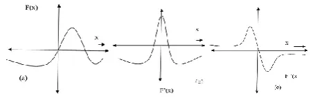
The image edge detection is increase the quality of computer vision, as it can locate significant property of images. For illustration, image edge is the processing of images to enhance their look to human analyzer or to enhance the performance of various images processing system. An edge detection algorithm incorporate 2 steps: first one is the “image enhancement” and second gathering information about the structural data of objects[10][11]. The image improvement estimates the pixel classification and image spatial derivatives, the classification of image pixel into two sets - non-edge and edge. There exist various methods to perform edge detection; however, the most of unlike method may be clubbed into two categories - transform domain and spatial domain. The transform procedure generally uses gradient method; the gradient method for edge detection is viewing for the minimum and maximum point in the Ist derivative of image. The Laplacian method [3] looks for zero crossing in the 2nd derivatives of the image to locate edge. 1- dimensional shape of a ramp an edge exhibits and calculating the derivatives of the image can illuminate its location, in other

manner transformation will "restructure" the image, when leaving transformation coefficients whose structure is simple to model. In actuality images are well defined by their singularity (ridge and edge) structures. The Fig. 3 shows a look of gradient value;

Fig. 3 (a) Wave function (b) First derivation of function (c) Second derivation of function

The Canny Edge Detection

The Canny edge detector algorithm with general application of software are extensively considered and the accepted edge detection algorithm in today’s industry. First developed by John Canny for his Master’s thesis at MIT in 1986 [4], and still exceed/outrun many of the current algorithms which has developed till today. Canny’s ambitionwas to unearth the optimal edge of image, the algorithm is known as “Canny edge detection algorithm” this algorithm is also called as optimal edge detector algo. Canny's idea was to increase the edge detection, at that time these techniques are already existed during the time when he begin his work in this area [4]. The max and first obvious benchmark is lower an error rate. It is necessary that edges existing in images should not be forgotten and that there should not be any acknowledgement to non edges. Canny took the edge detection issue as a signal processing optimization problem, so he created an objective function to be optimized. The Canny edge detection [7][15] is extensively used in computer vision to identify acute intensity variations and to locate object boundaries in an image. Canny edge detection is gradient based edge detection algorithm. By saying Canny algorithm optimal image edge detection, it is meant as “good localization”, “good detection”, and “minimal response”. Moreover, by applying Canny algorithm on an image, reduced noise is achieved without any virtual edge.

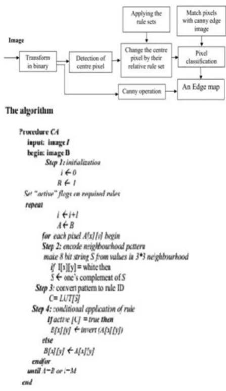
III. PROPOSEDMETHOD

The edge of any image is recognized by the certain rule sets. These rule sets are basically part of cellular automata which consists pixel as a cell and neighbour cells as neighbouring pixels. Cellular automata (CA) consist of regular grid of cells, each of which represents one of the finite numbers of possible states at a time. The state of cell is determined by the previous states of surrounding cells in discrete time steps.[13] These rule sets are applied on the binary image to find the point of sharp intensity changes in pixel value. The set of intensity- change-points are considered as an edge of the image. In this technique, there are 28 _{(=256) possible states of a pixel corresponding to} their neighbouring pixels.

can perform equivalent to other 50 operations. This rule is considered as ‘bestrule’.

In this paper, firstly the operation for edge detection is performed and then derived result is compared to different edge detection techniques. In first step find all 28 _{(= 256)} possible rule-set and remove the symmetry [13] by using 51 rule set operation for the edge detection. Finally, Sequential Floating Forward Search algorithm (SFFS) is applied to find the group of best rule set among the used rule sets on image for the edge detection. After applying SFFS, a single rule is achieved that is equivalent to other 51 rule sets at their respective points in image. Rule set and selection of best rule set. First section is considering block diagram.

Next is in about the explanation of algorithm and end with the selection of best rule set. The implementation has been done in Matlab and the image used in jpg,png etc image. The block diagram of this methodology is givenbelow,

At first before applying the algorithm,, the image, of which the edge are to be detected, should be in black and white. If the image not in the black and white convert it in to the back and white. The reason for using black and white image is if gray image are consider for edge detection then more number of rule set will be required which will be affect

In an image, edge displays sudden change in the intensity of pixels in comparison to neighbourhood pixels. This implies that pixels will be an edge pixels will be an edge pixels only when there is change in intensity to neighbourhood pixels. Now a pixels can have only 8 neighbourhood pixels whose centre pixels either black or white. In this way, for any 3*3 pixels matrix, 2^8 = 512 states are possible. If either of black or white pixels is consider the states will further reduced by half i.e. 256 state are possible. If there is 256 states are further analyses 8 fold symmetry can be found if this 8 fold symmetry is further removed then the possible state will steeply fall to 51 as shown in Fig.4. On the basis of frequency of rule set are being applied. Objective of the thesis is to reduced the number of rule sets are required

Before starting the algorithm a blank image of size equal to the input image is taken for the edge detection process, then each pixels of input image is matched again 51 rule sets the blank image taken is change accordingly. The pixels of image are taken in to left to right top to bottom fashion. If one of the pixels are matched one of the 51 rule set, a flag is set as in active state and next step of algorithm is followed, in second step the centre pixels of rule set matrix is copied to the blank image at the same co- ordinate as the input image.

This process goes on until all the pixels of input image are not covered. In this way, blank image will finally contain an edge image.

Fig. 4 Complete rule set containing 51 patterns.

Selection of Best Rule Sets

For the selection of rule sets apply an approach that is called “sequential floating forward algorithm”(SFFS); in this algorithm the choice of rule sets according to their objective function value. The 51 rule sets are applying one by one and their objective function value are store in dynamic array according their relative rule sets. If the objective function is set as zero then the entire rule sets are got the space in lookup table, and if the objective function is set on one then all the rule sets are got the space in to lookup table; so the value of objective function could be selected according their visualization of edge image[12]. This operation is perform by all rule sets which are in array, now for the better image edge this operation is perform up to image which have maximum edge or the edge image could not improved, so this last point is got by the maximum iteration rule sets. The selection of rule according to the SFFS, basic steps of this algorithm is presented below

ISSN: 2278-3075, Volume-8 Issue-7S2, May 2019

This algorithm is basically use for the selection or rule set in look up table. In Look Up table the rule set are got the space according their use and near matching with Canny’s edge image. That’s mean the value of objective function is

select for the edge detection rule sets. This process is follow up to the maximum value of iteration or if there is no change in the edge image. This algorithm is start from the first rule to last one. This selected the rule set for the look up table on the basis of objective function; if the objective functions value is increase then it should be consider and follow the next rule set again if next rule set is change the value of objective function then this is rule set is selected for the look up table. If this rule have no increment in objective function then this rule set is leave from the table and again this process is going up to the end of the image[14].

IV. RESULTSANALYSIS

In previous results some rules are better perform for the detection of lines, circle, cone type of image, now here some image are to be consider for the detection edge by the set of better rule sets,

The Rules are 2, 4, 8, 10, 11, 12, 14, 20, 21, 24, 33, 35, 36, 38, 39, 44, 45, 48, 49 and 50.

Now these rules are as shown in figure:-

V.CONCLUSION

It has been observed that the outcome for the edge detection through CA rules is motivating. As compared with the Canny operator the derive rule sets provides better edge

unmistakably showed in the outcome section. Fulfillment and use of CA rules is simple and clear in comparison of other existing algorithm such as Canny operator. The endeavor depicted in the thesis is restricted to binary images only and linear search method is used, the above Algorithm can be improved by altering for some gray scale images and other searching methods to improve the outcome.

REFERENCES

1. Zhou jun,Hu Qimei and He Xiangjian on ICITA 2004 ISBN 0-646-42313-4.

2. Vincent Torre and Tomaso A. Poggio, on edge detection IEEE Transactions On Pattern Analysis and Machine Intelligence. Vol. No 2, March1986.

3. Berzines V. Accuracy of Laplacian edge detectors, pp195-210,1984. 4. Canny John, A Computational Approach to edge Detection, IEEE

Transaction on Pattern analysis and Machine Intelligence, Vol. No 6, November 1986

5. Wolfram S. Cellular Automata and Complexity Collected Papers. Reading,MA:Addison-Wesley, 1994.

6. Kumar Tapas, Sahoo G. Kumar Tapas, Sahoo G. “A Novel Method of edge Detection using Cellular Automata” International journal of computer Application (0975-8887)Vol 9- No4 November2010.International journal of computer Application (0975-8887)Vol 9- No4 November 2010. 7. SOBEL, An Isotropic 3×3 Gradient Operator, Machine Vision for

Three – Dimensional Scenes, Freeman, H., Academic Pres, NY, 376-379,1990.

8. Joshi, S.R. ; Koju, R. “Study and comparison of edge detection algorithms” (AH-ICI),2012

9. Marr D. and Hildreth E., Theory of edge detection, proceeding of Royal Society, London. Vol. B207, pp.187-127,1980.

10. Grimson W.E.L and Hildreth E.C., Comments on “Digital steps edge from zero crossing of second directional derivatives, IEEE Transactions on Pattern Analysis and Machine Intelligence, Vol. PAMI-7,pp.121-129, Jan1985.

11. Rosin Paul L. “Training Cellular Automata for Image Processing”. IEEE Transactions on Image processing Vol. 15, No.7, July-2006. 12. Sarah Price, “Edges: The Canny Edge Detector”, July 4,1996. 13. James A.R. Marshall “Computational Method for Complex Systems”

Lecturer-8, Friday 13 Oct- 2008.