Parallel Data Mining for Medical Informatics
Xiaohong Qiu
UITS, Indiana University
501 N. Morton St., Suite 211
Bloomington, IN 47404
1-812-8550804
[email protected]
Geoffrey Fox
School of Informatics, Indiana
University 919 E. 10
thSt., Rm. 226A
Bloomington, IN 47405
1-812-8567977
[email protected]
ABSTRACT
As in many fields the data deluge impacts all aspects of Life Sciences from chemistry data in PubChem; genetic sequence data through health records. This data demands analysis and mining algorithms that are both high performance and robust. Further although some of the data can be usefully viewed as points in a vector space; for others it is better just to consider relationships defined just by dissimilarities between points. We develop parallel algorithms for both pairwise (no vectors) and vector based clustering using deterministic annealing for robustness and present preliminary results on medical record and gene sequence studies. We compare MPI and threading on multicore systems with up to 24 cores on an individual system and 128 cores on an 8 node cluster. In our analysis of performance and ease of programming, we note MPI is particularly effective in MapReduce scenarios and although threading is efficient at the times when MPI needs send and receive, it can have significant synchronization overhead due to runtime fluctuations on Windows.
Categories and Subject Descriptors
D.1.3 [Programming Techniques]: Parallel Programming – MPI,
Threading, CCR, multicore; I.5.3 [Pattern Recognition]: Clustering – Deterministic Annealing; J.3 [Life and Medical Sciences]; G.3 [Probability and Statistics] Statistical Software
General Terms
Algorithms, Performance
Keywords
Parallel and distributed algorithms, Software environments, Programming frameworks and language/compiler support.
1.
INTRODUCTION
Data intensive science is of growing importance as data volumes from instruments, sensors, digital documents and simulations increase exponentially in a trend that is expected to continue. This has prompted much research and large scale deployments for both science and particularly the commercial information retrieval field. In the Grid community such data intensive applications are typically implemented as workflows [1] while MapReduce [2] in Information Retrieval and Mashups [3] in a broad community represent related ways of integrating distributed data analysis or data mining filters. Such workflow, “MapReduction” or mash-up of filters is a successful paradigm and earlier we have suggested that it be extended to parallel computing. This implies that both parallel and distributed computing can be considered as orchestrations of coarse grain filters. This model applies to a Biologist using Taverna [1] to link Internet resources with a graphical interface or to composite signal processing system built
using Matlab with a scripting interface. As the data volumes grow, one needs to address the scalability of both the integrating workflow and the underlying filter. There are important cases where this straightforward. In particle physics the filters are pleasingly parallel over the underlying event dataset. In information retrieval, one supports independent data-parallel maps plus reductions. In such cases, scaling of the filters can be addressed using the workflow engine itself. However in general, one will need to parallelize the filters and this is problem discussed here. When the filters are linear algebra, one can straightforwardly scale using SCALAPACk or equivalent libraries. Matlab has also parallelized these and other algorithms. However many important algorithms are only available (as a service) in sequential form and so our project is identifying key data analysis algorithms and developing parallel versions. One typical example is “multiple sequence alignment” MSA (see reviews in [4] and [5] for example) where one takes sets of sequences and translates the component features to globally optimize their alignment. Here several implementation (for example CLUSTALW, MUSCLE, T-COFFEE and DIALIGN) are popular and available in open source fashion but only in sequential versions. Current progressive alignment algorithms scale like N4 for N sequences and a few thousand sequences take
We use C# on Windows platforms in our research as one of our motivations is to develop data mining software that can be used on future multicore clients. We also expect managed code (C#, Java) to be important in future analysis environments. This choice allows seamless environments stretching from a Windows client to backend high performance environments. In section 2 we discuss our hybrid MPI/Threading environment and the hardware platforms. Section 3 describes the PWDA and VECDA algorithms and their parallelization. Section 4 contains a preliminary performance analysis with results spanning individual 8, 16 and 24 core workstations with largest parallelism seen on a cluster of eight 16 core AMD Barcelona workstations. Our conclusions are in Section 5.
2.
PARALLEL SOFTWARE AND
HARDWARE ENVIRONMENTS
2.1
Hardware Systems
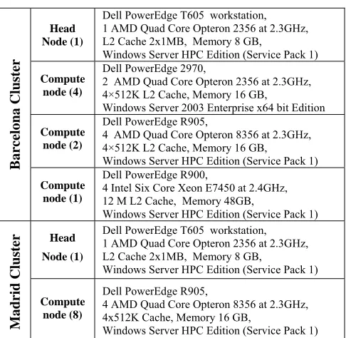
[image:2.612.55.298.360.597.2]There’re two set of clusters that provide different combinations of hardware system and serve as our test environments. The “Barcelona” cluster has increasing number of cores for compute nodes ─ four 8 core, two 16 core, and one 24 core. The “Madrid” cluster is a homogenous model that consists of eight 16 core compute nodes. Both clusters have quad-core AMD Opteron processor-based servers from Dell except for its latest 24 core model that uses 6-core Intel Xeon E7450 processor. Cluster nodes are connected by 1 GbE onboard NICs with 10 Gigabit switch.
Table 1. Machines used
Barcelona Cluster
Head Node (1)
Dell PowerEdge T605 workstation, 1 AMD Quad Core Opteron 2356 at 2.3GHz, L2 Cache 2x1MB, Memory 8 GB,
Windows Server HPC Edition (Service Pack 1)
Compute node (4)
Dell PowerEdge 2970,
2 AMD Quad Core Opteron 2356 at 2.3GHz, 4×512K L2 Cache, Memory 16 GB,
Windows Server 2003 Enterprise x64 bit Edition
Compute node (2)
Dell PowerEdge R905,
4 AMD Quad Core Opteron 8356 at 2.3GHz, 4×512K L2 Cache, Memory 16 GB,
Windows Server HPC Edition (Service Pack 1)
Compute node (1)
Dell PowerEdge R900,
4 Intel Six Core Xeon E7450 at 2.4GHz, 12 M L2 Cache, Memory 48GB,
Windows Server HPC Edition (Service Pack 1)
Madrid Cluster
Head
Node (1)
Dell PowerEdge T605 workstation, 1 AMD Quad Core Opteron 2356 at 2.3GHz, L2 Cache 2x1MB, Memory 8 GB,
Windows Server HPC Edition (Service Pack 1)
Compute node (8)
Dell PowerEdge R905,
4 AMD Quad Core Opteron 8356 at 2.3GHz, 4x512K Cache, Memory 16 GB,
Windows Server HPC Edition (Service Pack 1)
2.2
Software Environments
All the algorithms were explicitly written for arbitrary MPI and threading parallelism. As our software is C#, we used the MPI.NET (version 1.0) environment [15] which is a C# wrapper around Microsoft’s MPI and offers full functionality and performed excellently on our problems.
The Microsoft CCR (Concurrency and Computation Runtime) threading environment has been described in earlier papers [7-10]. We used version 2.0. We note that it is flexible and high
performance and easily supports two modes. In the first short lived threads are spawned dynamically and execute independent tasks before terminating at a synchronization point. In the second mode, we adopt a model where CCR threads [11,12] are used more like MPI processes and are long lived with rendezvous synchronization points from time to time. We term these the short-lived and long-lived threading modes in section 4.
In the hybrid model allowing both MPI and Threading, MPI is always used between nodes but each node can be any number of MPI processes that themselves run a set of threads. In the results given here, the product of the number of MPI processes per node and the number of threads per node was always less than equal to the number of cores on the node. Note that decreasing number of MPI processes, increases the message size and decreases the number of messages for a given problem/overall parallelism. This increases performance but in this case processing the message does not exploit the several cores available to each MPI process. We use the term parallel unit to refer to either thread or process in what follows. We let P be the total number of parallel units – this is number of MPI processes multiplied into the number of threads per process.
3.
CLUSTERING ALGORITHMS
3.1
Clustering Algorithms
Clustering can be viewed as a optimization problem that determines a set of K clusters by minimizing
HVEC = i=1Nk=1K Mi(k) DVEC(i,k) (1)
where DVEC(i,k) is the distance between point i and cluster center
k. Mi(k) is the probability that point i belongs to cluster k. This is
the vector version and one obtains the pairwise distance model with:
HPW = 0.5 i=1Nj=1N D(i, j) k=1K Mi(k) Mj(k) / C(k) (2)
and C(k) = i=1N Mi(k) is the expected number of points in the
k’th cluster. Equation (1) requires one be able to calculate the distance between a point i and the cluster center k and this is only
possible when one knows the vectors corresponding to the points
i. (2) reduces to (1) when one inserts vector formulae and drops
terms i=1N j=1N DVEC(i,k) DVEC(j,k) k=1K Mi(k) Mj(k) that average to zero.
We minimize (1) or (2) as a function of cluster centers (1) and cluster assignments Mi(k) (in both cases). One can derive
deterministic annealing from an informatics theoretic [13] or physics formalism [14]. In latter case one smoothes out the cost function (1) or (2) by averaging with the Gibbs distribution exp(-H/T). This implies in a physics language that one is minimizing not H but the free energy at temperature T and entropy S
F = H-TS (3)
For VECDA and Hamiltonian H given by equation (1), one can do this averaging exactly.
Mi(k) = exp( - DVEC(i,k)/T ) / Zi (4)
Zi = k exp( - DVEC(i,k)/T ) (5)
F = - T i=1N log [Zi] / N (6)
integrals are effectively performed by Monte Carlo. This implies simulated annealing is always applicable but is usually very slow. The applicability of deterministic annealing was enhanced by the observation in [14] that one can use an approximate Hamiltonian H0 and average with exp(-H0/T). For (2), one uses the form
motivated by the VECDA formalism (4).
H0 = i=1Nk=1K Mi(k) i(k) (7) Mi(k) exp( -i(k)/T ) with k=1K Mi(k) =1 (8)
i(k) are new degrees of freedom. This averaging removes local minima and is designed so that at high temperatures one starts with one cluster. As temperature is lowered one minimizes (3) with respective to degrees of freedom. A critical observation of Rose [13] allows one to determine when to introduce new clusters. As in usual expectation maximization (steepest descent) the first derivative of (3) is set to zero to find new estimates for Mi(k) or other parameters (cluster centers for VECDA). Then one
looks at the second derivative of F to find instabilities that are resolved by splitting clusters. One does not examine the full matrix but the submatrices coming from restricting to variations of the parameters of a single cluster with the K-1 other clusters fixed and two clusters placed at location of clusters whose stability one investigates. As temperature is lowered one finds that clusters naturally split and one can easily understand this from the analytic form for . The previous work [14] on PWDA was incomplete and did not consider calculation of but rather only assumed an a priori fixed number of clusters. We have completed the formalism and implemented it in parallel. Note we only need to find the single lowest eigenvalue of (restricted to varying one cluster). This is implemented as power (Arnoldi) method. One splits the cluster if its restricted has a negative eigenvalue and this is smallest – minimized over all clusters.
The formalism for VECDA can be found in our earlier work and [Rose98]. Here we just give results for the more complex PWDA and use it to illustrate both methods. We let indices k runs over clusters from 1 to K while i jrun over data points from 1
to N. Mi(k) has already been given in equation (8). Then one
calculates:
A(k) = - 0.5 i=1Nj=1N D(i, j) Mi(k) Mj(k) / C(k)2 (9a)
B(k) = i=1N D(i, ) Mi(k) / C(k) (9b)
C(k) = i=1N Mi(k) (9c)
Allowing the estimate (k) = (B(k) + A(k)) (10)
which minimizes F of equation (6). The NKNK second
derivative matrix is given by
{,}{,} = (1/T) {M() - M() M() } +
(M() M() / T2) {k=1K [- 2A(k) - B(k) - B(k) + D(,)]
[M(k) - k ] [M(k) - k]/C( k)} (11)
Equations (9) and (10) followed by (8) represent the basic steepest descent iteration that is performed at fixed temperature until the estimate for (k) is converged. Note steepest descent is a
reasonable approach for deterministic annealing as one has smoothed the cost function to remove (some) local minima. Then one decides whether to split a cluster from the eigenvalues of as discussed above. If splitting is not called for, one reduces the temperature and repeats equations (8) through (11). There is an elegant method of deciding when to stop based on the fractional freezing factors (k)
(k) = i=1N Mi(k) (1 - Mi(k)) / C(k) (12)
As temperatures are lowered after final split, then the Mi(k) tend
to either 0 or 1 so (k) tends to zero. We currently stop when all the freezing factors are < 0.002 but obviously this precise value is ad-hoc.
3.2
Multi-scale and Deterministic Annealing
Deterministic annealing can be considered as a multi-scale approach as quantities are weighted by exp (-D/T) for distances D and temperature T. Thus at a given temperature T, the algorithm is only sensitive to distances D larger than or of order T. One starts at high temperatures (determined by largest distance scale in problem) and reduce temperature (typically by 1% each iteration) until you reach either the distance scale or number of clusters desired. As explained in original papers [12], clusters emerge as phase transitions as one lowers the temperature and need not be put in by hand.
[image:3.612.320.542.254.437.2]3.3
Geometric Structure and Visualization
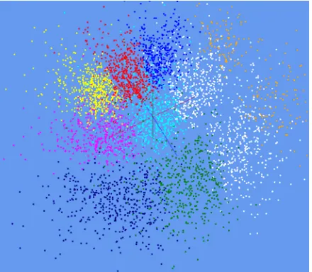
Figure 1. 4000 Patient Records with 8 clusters from PWDA
Figure 2. 4500 ALU pairwise aligned Gene Sequences with 10 clusters from PWDA
[image:3.612.320.540.456.648.2]with MDS [6] and visualizing with a 3D viewer written in DirectX. As a next step, we will allow users to select regions either from clustering or MDS and drill down into the substructure in this region. Like the simpler linear principal component analysis, MDS of a sub-region is generally totally different from that of full space. We note here that deterministic annealing can also be used to avoid local minima in MDS. We will report our extensions of the original approach in [18] and comparison with Newton’s method for MDS [19] elsewhere.
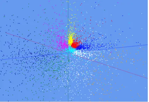
Figure 3. Gene Sequences data of Figure 2 mapped by a dimension reduction function before MDS.
Clustering in high dimensions d is not intuitive geometrically as the volume of a cluster of radius R is proportional to R(d+1)
implying that a cluster occupying 0.1% of total volume has a radius reduced by only a factor 0.99 from that of overall space with d=1000 (a value typical of gene sequences). These conceptual difficulties are avoided by the pairwise approach. One does see the original high dimension when projecting points to 3D for visualization as they tend to appear on surface of the lower dimensional space. This can be avoided as discussed in [22] by a mapping Distance D f(D) where f is a monotonic function designed so that the transformed distances f(D) are distributed
uniformly in a lower dL dimensional space. We experimented with
dL = 2 and 4 where the mapping is analytically easy but found it
not improve the visualization. Typical results are shown in figure 3 that maps data of figure 2 to 2 dimensions before applying MDS – the clustering is still performed on original unmapped data. Certainly the tendency in figure 2 to be at edge of visualization volume is removed but data understanding does not seem improved. This approach finds an effective dimension deff for
original data by comparing mean and standard deviation of all the inter-point distances D(i,j) with those in a dimension deff. This determines an effective dimension deff of 40-50 for sequence data
and about 5 for medical record data.; in each case deff is a dimension smaller than that of underlying vector space. This is not surprising as data is a very special correlated set of points.
3.4
Parallelism
The parallelism for clustering is straightforward data parallelism with the N points divided equally between the P parallel units. This is the basis of most MapReduce algorithms and clustering was proposed as a MapReduce application in [20]. We have in fact compared simple (K-means) clustering between versions and MapReduce and MPI in [21] and VECDA should be more suitable
for MapReduce as it is more computation at each iteration (MapReduce has greater overhead than MPI on communication and synchronization). VECDA only uses reduction, barrier and broadcast operations in MPI and in fact MPI implementation of this algorithm is substantially simpler than the threaded version. Reduction, Barrier and Broadcast are all single statements in MPI but require several statements – especially for reduction – in the threaded case. Reduction is not difficult in threaded case but requires care with many opportunities for incorrect or inefficient implementations.
PWDA is also data parallel over points and its O(N2) structure
gives it similarities to other O(N2) algorithms such as those for
particle dynamics. We divide the points between parallel units. Each MPI process also stores the distances D(i, j) for all points i
for which process is responsible. Of course the threads inside this process can share all these distances stored in common memory of a multicore node. There are subtle algorithms familiar from N-body particle dynamics where a factor of 2 in storage (and in computation) is saved by using the symmetry D(i, j) = D(j, i) but this did not seem useful in this case. The MPI parallel algorithm now needs MPI_SENDRECV to exchange information about the distributed vectors; i.e. one needs to know about all components of vectors Mi Bi and the vector Ai iterated in finding maximal eigenvectors. This exchange of information can be done with a ring structure as again used in O(N2) particle dynamics problems.
We measured the separate times in the four components of MPI – namely SENDRECV, Reduction, and Broadcast and only the first two are significant reaching 5-25% of total time with Broadcast typically less than 0.1% of execution time. SENDRECV is typically 2 to 3 times reduction but the latter is a non trivial overhead (often 5-10%).
3.5
Computational Complexity
The vector and pairwise clustering methods have very different and complementary computational complexities. VECDA execution time is proportional to N d2 for N points – each of
dimension d. PWDA has an execution time proportional to N2.
PWDA can rapidly become a supercomputer computation. For example with 4500 sequence datapoints and 8 clusters, the sequential execution time is about 15 hours on a core of the systems used in our benchmarks. A direct clustering with PWDA of half million points (relevant even today) would naturally use around 5000 cores (100 points per core) with pure MPI parallelization. The hybrid threading-MPI parallelism could support more cores as discussed in Sec 2.2.
We note that currently some 40-70% of the computation time is used in deciding whether to split clusters in PWDA; there are probably significantly better less time expensive algorithms here. The runs of VECDA reported here correspond to a low dimension space d = 2 for which negligible time is spent in splitting decision. The second derivative matrices are of size NKNK for PWDA and of size dKdK for VECDA. These are full matrices but as power method for determining maximal eigenvalues is used the computation is proportional to to the square of the matrix dimension. For computations reported here, the annealing uses from 1000-10,000 temperature steps while each eigenvalue determination uses 10-200 iterations.
We used three sample applications in the research reported here and expect other publications to address the domain specific scientific results. Here we just use them to study the algorithms and their performance. The first application was a collection of 1500, 3000 and 4500 ALU sequences where the clustering is designed to understand gene families as discussed before in [23]. Results from this are seen in figures 2 and 3 but not used in performance study. The second application came from medical informatics [24] and consisted of up to 36,000 medical records each of which had 30 properties connected to a study of childhood obesity. These properties were normalized uniformly and used to define a vector for each patient record consisting of continuous and binary data. These are combined to form a Euclidean distance between each patient record. As shown already in figure 1, this data shows striking structure after being clustered and projected by MDS to 3D. The third application was a Monte Carlo collection of ten Gaussian clusters in two dimensions; various dataset sizes were used and here we use results from datasets with 10 clusters – each containing 20,000 or 40,000 data points. We used the latter of scaled speedup studies of VECDA where problem size is increased proportional to the number of nodes. This is achieved by trivial replication of points as this ensures an execution time exactly proportional to the number of points. This is an artificial example but similar in architecture to the census data clustering reported in [8]
4.2
Approach
As in earlier papers [7-10], rather than plot speed-up, we present results in terms of an overhead f(n,P) where different overhead effects are naturally additive. Further in simple cases the overhead only depends on the grain size n = N/P in our case. Putting T(n,P)
as the execution time on P parallel units, we can define
Overhead f(n,P) = (PT(n,P)-T(Pn,1))/T(Pn,1) (13) and efficiency = 1/(1+f) and Speed-up = P (14)
We note that the overhead is approximately 1 – the efficiency .
4.3
Performance Results
[image:5.612.321.558.165.281.2]We obtain generally good speed-up (low overhead) in our measurements with however some surprising results.
Figure 4. Measurements of parallel overhead for samples of 2000 and 4000 element patient data on 8, 16 and 24 cores on a single workstation with thread-based parallelism
In figure 4, we show some simple runs on the 8, 16 and 24 core workstations in the Barcelona cluster of table 1. The highest overhead is 0.16 on 24 cores but even this corresponds to a
[image:5.612.321.553.435.638.2]speedup of 20.7 on the 24 core workstation. This data as expected (and seen in all our runs) shows the overhead increasing as data set sizes decrease. Figure 5 shows an effect that we will see in more detail later. This looks at execution time for a largish 10,000 element patient record data for different mechanisms for the parallelism. Namely we achieve 24 way parallelism (on the 24 core workstation) with different choices of MPI and threading.
Figure 5. 24 way parallel runs on 24 core Dell Intel workstation for different choices of MPI and Thread parallelism for 10,000 element patient data.
[image:5.612.57.265.487.630.2]The poorest performance is seen for the case of pure thread parallelism – 24 threads and no MPI (just the one process). This pure threading case is about 25% slower than the other choices – corresponding to 24 MPI processes(no extra threading), 12 MPI processes (each of 2 threads), 6 MPI processes (each of 4 threads), and finally 4 MPI processes (each of 6 threads). We have discussed the overhead of threading in our earlier papers and noted that Windows (the operating system used in all our results) has overheads that limit the speed up obtainable with threads.
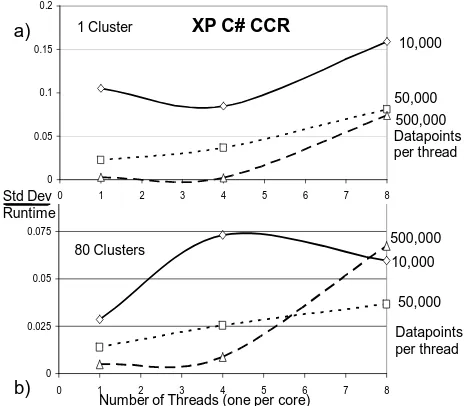
Figure 6. Measurements from [8] showing 5 to 10% runtime fluctuations on an 8 core workstation. The results are plotted as a function of number of simultaneous threads from 1 to 8 and for three different dataset sizes.
‐0.02 0 0.02 0.04 0.06 0.08 0.1 0.12 0.14 0.16 0.18
Patient2000‐16 Patient4000‐16 Patient2000‐8 Patient4000‐8 Patient4000‐24core
1 2 4 8 16 24 cores Overhead
0 0.025 0.05 0.075 0.1
0 1 2 3 4 5 6 7 8
Number of Threads (one per core)
80 Clusters 500,000
50,000 10,000
Datapoints per thread
b)
0 0.05 0.1 0.15 0.2
0 1 2 3 4 5 6 7 8
XP C# CCR
500,000 50,000
10,000
Datapoints per thread
a)
Std Dev Runtime
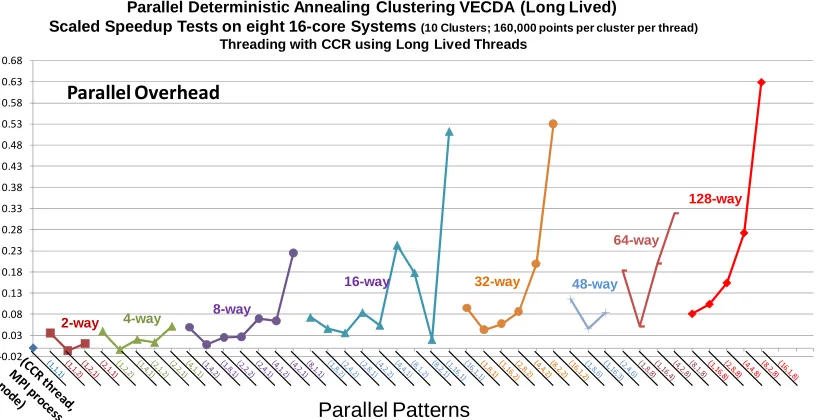
Figure 7. Parallel Overhead for VECDA using long lived threads run on 128 core Madrid Cluster in table 1. The results achieve a given parallelism by choosing number of nodes, MPI processes per node and threads per MPI process. The number of threads increases as you move from left to right for given level of parallelism.
In particular as discussed in [9], thread execution times fluctuate substantially with figure 6 showing standard deviations from 5 to 10% on a simple kernel representative of the VECDA clustering algorithm.
The identical code (translated from C# to C) shows order of magnitude lower fluctuations when run under Linux [ICCS] with interesting systematics even in Linux case. These fluctuations can give significant parallel overheads as parallel algorithms used in VECDA and PWDA like those in most scientific algorithms requires iterative thread synchronization at the rendezvous points. Here the execution time will be the maximum over that of all the simultaneous fluctuating threads and so increase as this number increases. As described in the earlier papers we have always seen this and reported this effect to Microsoft. We found that these fluctuations were the only sizeable new form of parallel overhead compared to those well known from traditional parallel computing i.e. in addition to load imbalance and communication overhead. We did note the possible of extra overheads due to different threads interfering on a single cache line but our current software is coded to avoid this. Note that the fluctuation effect is larger in the work reported here compared to our previous papers as we are looking here at many more simultaneous threads. Note that the effect does not just reflect the number of threads per process but also the total number of threads because the threads are synchronized not just within a process but between all processes as MPI calls will synchronize all the threads in the job. Thus it is interesting to examine this effect on the full 128 core Madrid cluster as this could even be a model for performance of future much larger core individual workstations.
Note that our current clusters of table 1 only have 10 gigabit Ethernet connections and we will extend our work with a new Infiniband connected 24 core node Windows cluster. This should
allow more sensitive examination of this thread synchronization problem. We note that VECDA and PWDA differ somewhat in this respect. VECDA only uses reduction (dominant use), broadcast and barrier MPI operations and so has particularly fast MPI synchronization. PWDA also has MPI_SENDRECV (exchange of data between processes) which increases the MPI synchronization time and could be expected to mask the thread synchronization effect.
We see an interesting demonstration of this effect in figure 7 which shows the parallel overhead for 44 different choices of nodes (from 1 to 8), MPI processes per node (from 1 to 16) and threads per node (from 1 to 16 divided by MPI processes per node). The results are divided into groups corresponding to a given total parallelism. For each group, the number of threads increases as we move from left to right. For example in the 128 way parallel group, there are five entries with the leftmost being 16 MPI processes per node on 8 nodes (a total of 128 MPI processes) and the rightmost 16 threads on each of 8 nodes (a total of 8 MPI processes). We find an incredibly efficient pure MPI version – an overhead of just 0.08 (efficiency 92%) for 128 way parallelism whereas the rightmost case of 16 threads has a 0.63 overhead (61% efficiency). All cases with 16 threads per node show a high overhead that slowly increases as the node count increases. For example the case of 16 threads on one node has an overhead of 0.51. Note that in this we use scaled speedup i.e. the problem size increases directly according to number of parallel units. This ensures that the inner execution scenarios are identical in all 44 cases reported in figure 7. We achieve this by replicating a base point set as one can easily see that leads to same mathematical problem but with a work that increases properly as number of execution units increases.
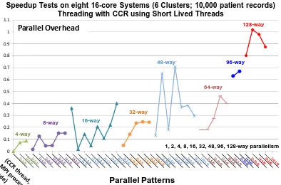
Figure 8 shows similar results for the execution of PWDA on the Madrid cluster for the Patient data set with 10,000 elements – the same one used in figure 5. Generally MPI parallelism outperforms thread parallelism but the effect is not as large as that in figure 7. Part if not all of this difference is due to the substantially higher MPI overhead which is largely due to MPI_SENDRECV which is not used in the VECDA parallel algorithm in figure 7.
Parallel Patterns
‐0.020.03 0.08 0.13 0.18 0.23 0.28 0.33 0.38 0.43 0.48 0.53 0.58 0.63 0.68
Parallel Deterministic Annealing Clustering VECDA (Long Lived)
Scaled Speedup Tests on eight 16-core Systems(10 Clusters; 160,000 points per cluster per thread)
Threading with CCR using Long Lived Threads
Parallel
Overhead
2-way 4-way
8-way
16-way 32-way 48-way 64-way
Figure 8. Parallel Overhead for PWDA run on 128 core Madrid Cluster in table 1. The results achieve a given parallelism by choosing number of nodes, MPI processes per node and threads per MPI process. The number of threads increases as you move from left to right for given level of parallelism.
The MPI overhead is such that this problem set size is best suited to systems with 64 or smaller levels of parallelism. For example for the cases of 16 MPI processes on 4 nodes or 8 MPI processes on 8 nodes, we find an overhead of 0.18 entirely described by MPI overheads (that were measured during run) that were 28% MPI_REDUCE and the remainder MPI_SENDRECV as broadcast time was negligible. The threaded implementations of 64 way parallelism have about twice the overhead of case where MPI is used on the node. Figure 8 shows more variation than figure 7 (see for example 48 way parallelism group) because we now see significant increase in overheads as we increase the number of nodes with the 6 node cases of 48 way parallelism showing more overhead than 3 node case. Our near future work includes improving the clarity of figures with extended patterns for runs, re-ordering within groups and improving statistics by averaging over several runs for each scenario.
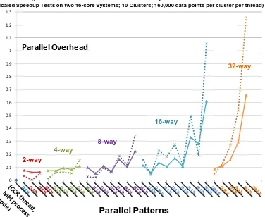
To investigate this effect further we carefully re-implemented the VECDA code replacing long threads by short lived threads spawned at each new parallel section. In figure 9, we compare the two versions of VECDA on the Barcelona cluster of table 1. The results have similar structure to figure 7 except the long lived VECDA-LL code (solid lines) has lower overheads than the newer short lived thread VECDA-SL code (dotted lines). We had hoped that the high overheads seen in figures 7, 8 and 9 for patterns with many threads might have been some glitch in the rather tricky long lived code. However our results support the correctness of the original code and suggest that as expected it is better to use long lived threads. This short lived threading
approach was also used in all PWDA results presented here but the results of figure 9 suggest that we should re-implement with long lived threads and use that choice in our ongoing work.
5.
CONCLUSIONS
We believe that libraries or collections of services implementing the best available algorithms in high performance parallel versions will be essential for many fields to exploit the data deluge. Our work has presented two complementary approaches to clustering – pairwise and vector based that together cover a broad range of problems. We have shown good parallel performance with as expected a given problem size running well up to a certain level of parallelism. We have shown significant impact on performance of different implementations. MPI outperforms threaded codes on Windows while a long lived threading with rendezvous synchronization outperforms a simpler model with short lived threads spawned afresh at each parallel section.
6.
ACKNOWLEDGMENTS
We thank other members of the SALSA parallel computing group for conversation and to Huapeng Yuan who developed some of the initial code – especially VECDA using long lived threads. Our work on patient data would not have been possible with Gilbert Liu from IU Medical School and the gene sequence data was produced by Haixu Tang and Mina Rho from the IU Bioinformatics group who also answered our endless naïve questions. The IU MPI.NET group led by Andrew Lumsdaine was very helpful as we learnt how to use this. This research was partially supported by Microsoft. We have obtained continued help on CCR from George Chrysanthakopoulos and Henrik Frystyk Nielsen. Scott Beason provided key support on visualization and set up of Clusters.
Parallel Pairwise Clustering PWDA
Speedup Tests on eight 16-core Systems (6 Clusters; 10,000 patient records)
Threading with CCR using Short Lived Threads
Parallel Overhead
0 0.1 0.2 0.3 0.4 0.5 0.6 0.7 0.8 0.9 1 1.1
4-way
8-way 16-way
32-way
48-way
64-way
128-way
96-way
1, 2, 4, 8, 16, 32, 48, 96, 128-way parallelism
Figure 9. Parallel Overhead for VECDA using long lived threads (solid) or short lived threads (dotted lines) run on 32 core Barcelona Cluster in table 1. The results achieve a given parallelism by choosing number of nodes, MPI processes per node and threads per MPI process. The number of threads increases as you move from left to right for given level of parallelism.
7.
REFERENCES
[1] Dennis Gannon and Geoffrey Fox, Workflow in Grid Systems Concurrency and Computation: Practice &
Experience 18 (10), 1009-19 (Aug 2006), Editorial of special issue prepared from GGF10 Berlin.
[2] Jeffrey Dean and Sanjay Ghemawat, MapReduce: Simplified Data Processing on Large Clusters, OSDI'04: Sixth
Symposium on Operating System Design and Implementation, San Francisco, CA, December 2004. [3] Geoffrey Fox and Marlon Pierce Grids Challenged by a Web
2.0 and Multicore Sandwich Special Issue of Concurrency&Compuitation:Practice&Experience on Seventh IEEE International Symposium on Cluster
Computing and the Grid — CCGrid 2007, Keynote Talk Rio de Janeiro Brazil May 15 2007
http://grids.ucs.indiana.edu/ptliupages/publications/CCGridD ec07-Final.pdf
[4] Julie D. Thompson, Frederic Plewniak and Oliver Poch, A comprehensive comparison of multiple alignment programs, Nucleic Acids Research 27, 2682-2690 (1999)
[5] Robert C. Edgar, MUSCLE: a multiple sequence alignment method with reduced time and space complexity, BMC Bioinformatics 5, 113 (2004)
[6] Seung-Hee Bae Parallel Multidimensional Scaling Performance on Multicore Systems at workshop on Advances in High-Performance E-Science Middleware and Applications in Proceedings of eScience 2008 Indianapolis IN December 7-12 2008
http://grids.ucs.indiana.edu/ptliupages/publications/eScience 2008_bae3.pdf
[7] Xiaohong Qiu, Geoffrey Fox, H. Yuan, Seung-Hee Bae, George Chrysanthakopoulos, Henrik Frystyk Nielsen High Performance Multi-Paradigm Messaging Runtime Integrating Grids and Multicore Systems September 23 2007 published in proceedings of eScience 2007 Conference Bangalore India December 10-13 2007
http://grids.ucs.indiana.edu/ptliupages/publications/CCRSept 23-07eScience07.pdf
[8] Xiaohong Qiu, Geoffrey C. Fox, Huapeng Yuan, Seung-Hee Bae, George Chrysanthakopoulos, Henrik Frystyk Nielsen PARALLEL CLUSTERING AND DIMENSIONAL SCALING ON MULTICORE SYSTEMS Invited talk at he 2008 High Performance Computing & Simulation
Conference (HPCS 2008) In Conjunction With The 22nd EUROPEAN CONFERENCE ON MODELLING AND SIMULATION (ECMS 2008) Nicosia, Cyprus June 3 - 6, 2008; Springer Berlin / Heidelberg Lecture Notes in Computer Science Volume 5101/2008 "Computational
0 0.1 0.2 0.3 0.4 0.5 0.6 0.7 0.8 0.9 1 1.1 1.2 1.3
Parallel Deterministic Annealing Clustering VECDA
Long Lived (LL solid lines) vs. Short Lived (SL dotted lines) Threads
(Scaled Speedup Tests on two 16-core Systems; 10 Clusters; 160,000 data points per cluster per thread)
4-way
8-way
2-way
32-way
16-way
Parallel
Overhead
Science: ICCS 2008" ISBN 978-3-540-69383-3 Pages 407-416 DOI: http://dx.doi.org/10.1007/978-3-540-69384-0_46 [9] Xiaohong Qiu, Geoffrey C. Fox, Huapeng Yuan, Seung-Hee Bae, George Chrysanthakopoulos, Henrik Frystyk Nielsen Performance of Multicore Systems on Parallel Data Clustering with Deterministic Annealing ICCS 2008: "Advancing Science through Computation" Conference; ACC CYFRONET and Institute of Computer Science AGH University of Science and Technology Kraków, POLAND; June 23-25, 2008. Springer Lecture Notes in Computer Science Volume 5101, pages 407-416, 2008. DOI: http://dx.doi.org/10.1007/978-3-540-69384-0_46
[10]Xiaohong Qiu , Geoffrey C. Fox, Huapeng Yuan, Seung-Hee Bae, George Chrysanthakopoulos, Henrik Frystyk Nielsen Parallel Data Mining on Multicore Clusters 7th International Conference on Grid and Cooperative Computing GCC2008 Shenzhen China October 24-26 2008
http://grids.ucs.indiana.edu/ptliupages/publications/qiu-ParallelDataMiningMulticoreClusters.pdf
[11]Home Page for SALSA Project at Indiana University http://www.infomall.org/salsa.
[12]Kenneth Rose, Eitan Gurewitz, and Geoffrey C. Fox Statistical mechanics and phase transitions in clustering Phys. Rev. Lett. 65, 945 - 948 (1990)
[13]Rose, K. Deterministic annealing for clustering, compression, classification, regression, and related optimization problems, Proceedings of the IEEE Vol. 86, pages 2210-2239, Nov 1998
[14]T Hofmann, JM Buhmann Pairwise data clustering by deterministic annealing, IEEE Transactions on Pattern Analysis and Machine Intelligence 19, pp1-13 1997 [15]MPI.NET Home Page
http://www.osl.iu.edu/research/mpi.net
[16]Microsoft Robotics Studio is a Windows-based environment that includes end-to-end Robotics Development Platform, lightweight service-oriented runtime, and a scalable and extensible platform. For details, see
http://msdn.microsoft.com/robotics/
[17]Georgio Chrysanthakopoulos and Satnam Singh “An Asynchronous Messaging Library for C#”, Synchronization and Concurrency in Object-Oriented Languages (SCOOL) at OOPSLA October 2005 Workshop, San Diego, CA. [18]Hansjorg Klock, Joachim M. Buhmann Multidimensional
scaling by deterministic annealing (1997) in Energy Minimization Methods in Computer Vision and Pattern Recognition, Eds Pelillo M. and Hancock E.R., Proc. Intl. Workshop EMMCVPR Venice Italy, Springer Lecture Notes in Computer Science 1223 ppg. 246-260 May 1997
[19]Anthony J. Kearsley, Richard A. Tapia, Michael W. Trosset The Solution of the Metric STRESS and SSTRESS Problems in Multidimensional Scaling Using Newton’s Method, technical report 1995.
[20]C. Chu, S. Kim, Y. Lin, Y. Yu, G. Bradski, A. Ng, and K. Olukotun. Map-reduce for machine learning on multicore. In B. Scholkopf, J. Platt, and T. Hoffman, editors, Advances in Neural Information Processing Systems 19, pages 281–288. MIT Press, Cambridge, MA, 2007.
[21]Jaliya Ekanayake, Shrideep Pallickara, and Geoffrey Fox Map-Reduce for Data Intensive Scientific Analyses Proceedings of the IEEE International Conference on e-Science. Indianapolis. 2008. December 7-12 2008
http://grids.ucs.indiana.edu/ptliupages/publications/ekanayak e-MapReduce.pdf
[22]Hansjorg Klock, Joachim M. Buhmann, Data visualization by multidimensional scaling: a deterministic annealing approach, Pattern Recognition 33 (2000) 651}669
[23]Alkes L. Price, Eleazar Eskin and Pavel A. Pevzner, Whole-genome analysis of Alu repeat elements reveals complex evolutionary history. Genome Res. 2004 14: 2245-2252 DOI: http://dx.doi.org/10.1101/gr.2693004