Robust methods for outlier detection and regression for SHM applications.

Robust methods for outlier detection and regression

for SHM applications

Nikolaos Dervilis*, Ifigeneia Antoniadou,

Robert J. Barthorpe, Elizabeth J. Cross and

Keith Worden

Dynamics Research Group,

Department of Mechanical Engineering, University of Sheffield,

Mappin Street, Sheffield S1 3JD, England, UK

Email: [email protected] Email: [email protected] Email: [email protected] Email: [email protected] Email: [email protected] *Corresponding author

Abstract: In this paper, robust statistical methods are presented for the data-based approach to structural health monitoring (SHM). The discussion initially focuses on the high level removal of the ‘masking effect’ of inclusive outliers. Multiple outliers commonly occur when novelty detection in the form of unsupervised learning is utilised as a means of damage diagnosis; then benign variations in the operating or environmental conditions of the structure must be handled very carefully, as it is possible that they can lead to false alarms. It is shown that recent developments in the field of robust regression can provide a means of exploring and visualising SHM data as a tool for exploring the different characteristics of outliers, and removing the effects of benign variations. The paper is not, in any sense, a survey; it is an overview and summary of recent work by the authors.

Keywords: structural health monitoring; SHM; environmental and operational influences; leverage points; outliers; novelty detection.

Reference to this paper should be made as follows: Dervilis, N., Antoniadou, I., Barthorpe, R.J., Cross, E.J. and Worden, K. (2015) ‘Robust methods for outlier detection and regression for SHM applications’, Int. J. Sustainable Materials and Structural Systems, Vol. 2, Nos. 1/2, pp.3–26.

Ifigeneia Antoniadou is a Lecturer in the Aerospace course of the Department of Mechanical at the University of Sheffield. Her first degree is in Electrical Engineering and Computer Engineering from the Aristotle University of Thessaloniki. After completing her PhD in Mechanical Engineering at the University of Sheffield, on the topic of structural health and condition monitoring of offshore wind turbines, she continued her work as a Research Associate at the same department with research focus on system identification and information extraction tools for decision-based design of engineering models. Her current research interests are on various aspects of data analysis and dynamics. She has published more than 32 papers in reputed journals and conferences.

Robert J. Barthorpe is a Lecturer in the Dynamics Research Group at the University of Sheffield. He received his MEng in Mechanical Engineering with German from the University of Sheffield in 2005 and completed his PhD degree in the field of data- and model-based approaches to structural health monitoring in 2010. His research includes interests in both damage identification and the verification and validation of numerical models, with a particular interest in the developing the tools required for ascribing credibility to model predictions.

Elizabeth J. Cross is a Senior Lecturer in the Dynamics Research Group in the Department of Mechanical Engineering. She received her first class degree in Mathematics from the University of Sheffield in 2007 and her MSc (Res.) with distinction in Advanced Mechanical Engineering, also from the University of Sheffield, in 2008. In 2012, she completed her PhD on Structural Health Monitoring whilst also working as a Research Associate in her final year in collaboration with Messier-Bugatti-Dowty. Her specific areas of interest include the development of robust models and indicators for structural performance and condition and the importation of sophisticated mathematical techniques for use in the disciplines of structural dynamics.

Keith Worden is a Professor in the Dynamics Research Group in the Department of Mechanical Engineering. In the dim and distant past, he received his BSc in Theoretical Physics from the University or York, eventually followed by a PhD in Mechanical Engineering from Heriot-Watt University. His primary research interests are in the application of techniques from machine learning and probability theory to problems in structural dynamics.

1 Introduction

The higher levels of SHM diagnostics – localisation, classification, severity assessment – are only accessible using supervised learning in the data-based approach (Farrar and Worden, 2012). In terms of damage detection the classification of a selected feature as abnormal or not is typified by two different approaches: supervised learning or unsupervised learning (novelty detection in this context). In terms of the SHM field, supervised learning means any procedure of classification of a feature which is trained with measurements representing and labelled by all conditions of interest (Dervilis et al., 2014a). Unfortunately, one does not often have data from damaged structures; this forces a dependence on unsupervised learning i.e. novelty detection. This means that detection is sensitive to benign EOVs in or around the structure. The premise of novelty detection is to seek the answer to the question if given newly presented data from the structure, do they come from its undamaged state? This is a vital point, as the measured responses from a structure and the extracted features that are sensitive to damage are usually also sensitive to any change in EOVs.

There is a need to find, visualise and remove such effects from feature data in order to prevent false alarms from diagnostic algorithms. Detecting EOVs is difficult because they manifest as multiple outliers – this requires robust methods of outlier/novelty detection. Unfortunately, this applies to both EOVs and data from a damaged system and a two-stage procedure is needed before monitoring: identify EOVs in training data and remove EOVs by subtraction or projection (Dervilis et al., 2014b, 2015).

Different methods have been investigated in order to handle the influence of external variations such as principal component analysis, auto-associative neural networks or, more recently, cointegration (Cross, 2012; Cross et al., 2011). These algorithms present a number of advantages and disadvantages in terms of their ability to remove benign conditions; however, in terms of characterising which of the outliers are labelled as ‘good’ in terms of detecting environmental/operational variations and which are ‘bad’ in terms of detecting structural degradation, very little effort has been carried out.

As mentioned, the problem is that EOVs in training data will manifest as many outliers and will be hard to detect because of ‘masking’ effects where multiple outliers conspire to hide each other. Recently developed robust methods allow effective detection of multiple outliers. Furthermore, a combined approach of robust regression and robust multivariate statistics can be exploited as a means of characterising and distinguishing the influence of environmental and operational conditions on the structural response. It will be shown via the successful implementation of robust regression analysis that environmental and operational conditions can be made to manifest themselves differently compared to the damage condition (Dervilis et al., 2014b, 2015).

This paper will discuss the performance of robust outlier and regression analysis for SHM purposes. The paper is not intended as a survey in any sense; it is simply an overview of recent work by the authors. The paper is justified here by the fact that the methods proposed should be considered as a coherent overview of a contribution to SHM.

2 Problem description

Outlier detection methods have been used for various applications over many years and cover a broad range of fields of research such as econometrics, computer sciences, medical and biological sciences, meteorology and even political science. One of the standard references is Barnett and Lewis (1984). Some recent advances regarding robust outlier detection can be found in Dervilis et al. (2014b, 2015), Hubert and Debruyne (2010), Schyns et al. (2010), Attar et al. (2013), Rousseeuw and Hubert (2013), Nurunnabi et al. (2012), Verdonck et al. (accepted), Fritsch et al. (2011), and Variyath and Vattathoor (2013).

There are several definitions as to what is an outlier. Hawkins (1980) and Barnett and Lewis (1984) give two general definitions. Barnett and Lewis indicate that “an outlying observation, or outlier, is one that appears to deviate markedly from other members of the sample in which it occurs”. Hawkins defines an outlier “as an observation that deviates so much from other observations as to arouse suspicion that it was generated by a different mechanism”. According to Hawkins (1980), mechanisms such as heavy-tailed distributions (like the t-distribution) or data that are coming from different kinds of distributions are often responsible for the contamination of data with outliers.

The classic discordancy measure for indicating outliers, as used in many of the previous studies, is the Mahalanobis squared-distance (MSD), which is given by the following equation,

{ }

{ }

(

)

(

{ }

{ }

)

2 T_[Σ]1

i x i x

i

D ₌ x ₋ μ − x ₋ μ ₍₁₎

where {xi} is the potential outlier, {μx} is the mean of the sample observations and [Σ] is the sample covariance matrix. The MSD tells one how far away a specific measurement is from the centre of the training data cloud, relative to the size of the cloud (Dervilis et al., 2014b, 2015). The mean and covariance matrix could be inclusive or exclusive measures; that is to say that the statistics may or may not have been computed from data where outliers are already present (Dervilis et al., 2014b, 2015). Generally, in many different fields the training data are not known a priori to be uncontaminated and an inclusive approach is a necessity. However, in the context of SHM or condition monitoring this situation presents a series of drawbacks regarding the use of multivariate statistics.

The main disadvantage of the classical distance measures (like the (MSD)) is that they can suffer from a multiple outlier ‘masking effect’ (Dervilis et al., 2014b, 2015). If there were groups of outliers already present in the training data, they would have a critical influence on the sample mean and covariance in such a way that they would subsequently indicate small distances on new observations or outlying data and thus cause the outliers to become hidden. The arithmetic mean and unbiased covariance matrix are statistics that suffer heavily from multiple outliers present in the data; they are not robust statistics. Specifically, when outliers from a cluster cloud that lie inside the data are present, they will directly move the arithmetic mean towards them and even expand the classical tolerance ellipsoid in their direction (Leroy and Rousseeuw, 1987).

the training data. This algorithm has already been used in an SHM context in Dervilis et al. (2014b, 2015).

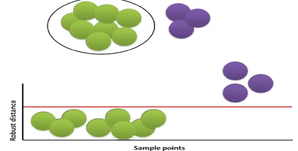
To make clear to the reader, the significant importance of the MCD against the MSD, in simple terms, is that the former allows one to search inclusively for multiple outliers by removing their ‘masking effect’ and revealing in multivariate data their infectious presence. A simple pictorial representation of this-supplementing the theory to follow – can be seen in Figures 1–2. The threshold calculation is described in Dervilis et al. (2014b, 2015).

Figure 1 Multiple outlier detection using MSD; the masking effect (see online version for colours)

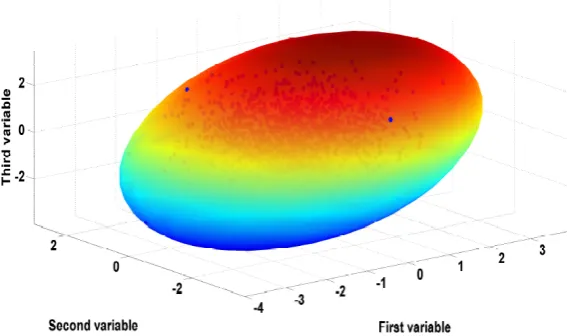
Figure 2 Multiple outlier detection using MCD (see online version for colours)

3 Robust estimators for distance measures

like the minimum volume enclosing ellipsoid (MVEE) and the phase-space thresholding method. As discussed in the introduction, robust outlier statistics are focussed mainly on a high level estimation of the ‘masking effect’ of inclusive outliers, not only for determining the presence or absence of novelty but also to examine the normal condition training set for multiple abnormalities.

3.1 Multiple outlier detection using the MCD estimator

The computation of the MCD estimator requires an extensive calculation. The FAST-MCD algorithm is implemented here as it is computationally efficient (Leroy and Rousseeuw, 1987; Rousseeuw and Van Driessen, 1999; Verboven and Hubert, 2005; Hubert et al., 2008; Rousseeuw and Van Zomeren, 1990; Jackson and Chen, 2004). The algorithm is given in detail in Leroy and Rousseeuw (1987), Rousseeuw and Van Driessen (1999), Verboven and Hubert (2005), Hubert et al. (2008), Rousseeuw and Van Zomeren (1990), and Jackson and Chen (2004), and the code adopted here was provided via a statistical Matlab library called LIBRA (Verboven and Hubert, 2005). A brief description of the algorithm FAST-MCD is provided here for the sake of completeness of the current paper.

A multivariate data matrix [X] = ({x1},…,{xm})T is assumed of m points in an

n-dimensional observation space (n × m) where {xi} = (xi1,…,xin)T is the observation. Robust estimates of the centre μ and the scatter matrix σ of X can be calculated by the MCD estimator. The MCD tool looks for the _h(_>m₂) _{observations out of m whose}

classical covariance matrix has the lowest possible determinant. The raw MCD estimate of location (arithmetic mean) is then computed from the average of these h points and the raw MCD estimation of scatter is the covariance matrix multiplied by a consistency factor (Dervilis et al., 2014b, 2015).

The calculation of the lowest determinant is vital as one moves from one approximation of MCD to another one with lower determinant. This property and the proof that follows it are not obvious and can be found in the appendix of Rousseeuw and Van Driessen (1999).

Based on the raw MCD estimates, a reweighting step can be added in order to increase the finite sampling efficiency. The advantage is that MCD estimates can resist up to (m – h) outliers and in turn, the number h (or equally h)

m

a= controls the robustness of the estimator. The highest resistance compared to contamination is achieved by calculating ( 1)

2 .

n m

h= + + It is proposed that when a large proportion of contamination is assumed then h = an with a = 0.5. Detecting outliers can be challenging when m / n is small because some data points can become coplanar. This is a general problem in the machine learning community called the ‘curse of dimensionality’. It is recommended (Verboven and Hubert, 2005) that when m 5,

n > a should be 0.5. Generally, the MCD estimates of location and scatter are affine equivariant which means that they are invariant under affine transformation behaviour (simultaneous rotation and translation). This is crucial as the underlying model is then immune to different variable scales and data rotations. Rousseeuw and Van Driessen (1999) developed the FAST-MCD algorithm based on a Concentration step (C-step). C-steps select the h

3.2 An example: Piper Tomahawk aircraft wing experiment

In the illustration given here, the experimental structure presented is an aluminium aircraft wing (Dervilis et al., 2014b, 2015). The wing is mounted in a cantilevered fashion on a substantial, sand-filled steel frame. Fifteen PCB piezoelectric accelerometers were mounted on the upper (as mounted) surface of the wing using ceramic cement. The sensors are denoted S1 to S15. Experimental data acquisition was performed using a DIFA SCADAS III system controlled by LMS software. All measurements were recorded within a frequency range of 0–2,048 Hz with a resolution of 0.5 Hz. The structure was excited with a band-limited white Gaussian signal using a Gearing and Watson amplifier and shaker mounted beneath the wing.

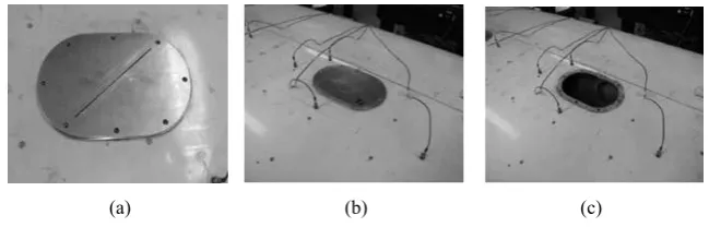
Damage was introduced in a repeatable manner by modifying the inspection panels on the underside of the wing. Five panels were considered and all of them had the same dimensions and orientation (Figures 3–5). The test sequence was arranged into two rounds of five blocks resulting in ten blocks. Each block contains three runs: a normal condition run, a damage (saw-cut) run and a damage (panel-off) run. Each run contains 100 observations. Within each block, only the panel of interest is removed or saw-cut panel replaced, the remaining four panels remain in place. In turn, at the end of the first run all five panels were removed and the second run started by repeating the procedure sequence again (Dervilis et al., 2014b, 2015).

Figure 3 Piper Tomahawk aircraft wing

Figure 4 Inspection panel in (a) normal condition, (b) removed panel and (c) saw cut

Figure 5 Schematic sensor placement diagram

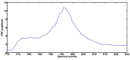
The region around the resonance frequency between spectral points 780–820 was used as a feature (see Figure 6). It is obvious that several feature combinations can be tested, by combining the normal condition with each panel removal and each of the sensor measurements in order to check the sensitivity of damage detection regarding the position of the sensor (for more results see Dervilis et al., 2014b).

Figure 6 Resonance frequency selected as a feature with 50 points around the peak (see online version for colours)

7700 775 780 785 790 795 800 805 810 815 820 825

2 4 6 8 10 12

Spectral points

FRF amplitude

Source: Dervilis et al. (2014b, 2015)

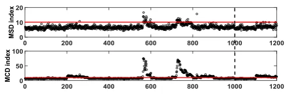
In the results that are shown in Figures 7–10 as an example the first 1,000 samples include the natural, undamaged condition of the structure of the ten blocks (ten blocks per diagram); the next 200 samples include either the panel removal (100 samples for each different run) or 200 samples include the panel saw cut damage (100 samples for each different run).

Figure 7 Novelty detection of normal condition of sensor 1 (see online version for colours)

0 100 200 300 400 500 600 700 800 900 1000 MCD index 0

50

0 100 200 300 400 500 600 700 800 900 1000 MSD index 0

10 20

Source: Dervilis et al. (2014b, 2015)

Figure 8 Novelty detection of normal condition of sensor 5 (see online version for colours)

0 100 200 300 400 500 600 700 800 900 1000 MCD index 0

50

0 100 200 300 400 500 600 700 800 900 1000 MSD index 0

10 20

Source: Dervilis et al. (2014b, 2015)

Figure 9 Novelty detection of sensor 14 in respect to panel 3, including panel removal (see online version for colours)

0 200 400 600 800 1000 1200

MCD index 0 20

400 200 400 600 800 1000 1200 MSD index 0

10 20

Source: Dervilis et al. (2014b, 2015)

Figure 10 Novelty detection of sensor 15 in respect to panel 1, including panel removal (see online version for colours)

0 200 400 600 800 1000 1200 MCD index 0

50 100

0 200 400 600 800 1000 1200 MSD index 0

10 20

3.3 Ellipse methods for outlier detection

In the same spirit as the MCD, other methods of finding minimum ellipses can be utilised in terms of outliers detection. Khachiyan (1996), Khachiyan and Todd (1993), Kumar and Yildirim (2005), Moshtagh (2005) and Sun and Freund (2004) established a linear-time reduction of the MVEE problem to the problem of computing a maximum volume inscribed ellipsoid (MVIE) in a polytope described by a finite number of inequalities (Dervilis et al., 2014b, 2015). Therefore, the MVEE problem can also be solved using the algorithms developed for the MVIE problem. Consider a set of m points in an

n-dimensional space: S = {{x1}…{xm}} ∈ Rn. Denote the MVEE of the set S by

MVEE(S). The ellipsoid should have positive volume and in centre form is given by Moshtagh (2005):

(

)

(

)

{

}

E= x ∈R x − c A x − c ≤ (2)

where {c} ∈Rn _{is the centre of the ellipse E and [A] ∈ S}n

++ (which is the set of n × n

positive definite matrices), describes the axes. The points {xi{ of the multivariate set S should each satisfy the constraint:

{ }

(

)

(

{ }

)

The volume of E which will be minimised is given by Moshtagh (2005),

( )

(

)

1/2

0 1

0

( ) det [ ]

det [ ]

u

vol E u A

A

− −

= = (4)

where u0 is the volume of the unit hypersphere in dimension n. In summary, the problem

of determining the ellipsoid of least volume containing the points of S is equivalent to finding a vector {c} ∈ Rn _{and an n × n positive definite symmetric matrix [A] which} minimises det([A]–1_{) subject to the constraint (3). The natural formulation of the problem}

is:

By varying [A], {c}, minimise det([A]–1_{) subject to the constraints:}

{ }

(

)

(

{ }

)

There are several different methods available in order to obtain a solution of the problem; the one used here is the dual formulation method based on Khachiyan’s algorithm (Dervilis et al., 2014b, 2015; Khachiyan, 1996; Kumar and Yildirim, 2005; Moshtagh, 2005; Sun and Freund, 2004). The discordancy test is similar to that given for the equation of the MCD or MSD and calculates the squared distance from the centre of the ellipse to each data vector.

Figure 11 Error 0.1 in the solution of MVEE with respect to the optimal value (tolerance) (see online version for colours)

Figure 12 Error 0.001 in the solution of MVEE with respect to the optimal value (tolerance) (see online version for colours)

In order to visualise the performance of the latter method, experimental gearbox vibration data from a wind turbine is displayed (Antoniadou and Worden, 2014; Antoniadou, 2013). The gearbox consists of three gear stages: one planetary gear stage and two spur gear stages. Before applying the phase-space thresholding tool, a time-frequency analysis is utilised, by implementing empirical mode decomposition (EMD) to the vibration data. The signals were decomposed into a set of signal components (oscillatory functions) in the time-domain called intrinsic mode functions (IMFs). In Figures 13–14, outlier detection using the phase-space threshold and the corresponding ellipsoid can be seen directly on the time series data formed from the instantaneous power of the second IMF.

Figure 13 Constructed ellipsoid in 3D phase space for the power of the second IMF (see online version for colours)

Source: Antoniadou and Worden (2014) and Antoniadou (2013)

Figure 14 Outlier detection using the phase-space threshold method for the power of the second IMF (see online version for colours)

0 360 720 1080 1440

0 1 2 3 4x 10

7

Gear Rotation [deg]

Power

Source: Antoniadou and Worden (2014) and Antoniadou (2013)

4 Regression estimators

Many regression estimators break down in the presence of outliers. Generally, there are also different kinds of outliers from those previously considered in this paper. Via a

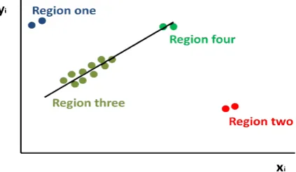
Generally, in linear regression analysis the studied examples of data are of the type ({xi}, {yi}) where {xi} is an m-dimensional input vector and the response {yi} is often a one-dimensional vector (Leroy and Rousseeuw, 1987; Rousseeuw and Van Zomeren, 1990). Cases for which an {xi} is far away from the majority of the {xi} observations are called leverage points.

If ({xi}, {yi}) is a leverage point then this indicates the ‘outlyingness’ of {xi}, but does not take into account the regression response {yi} (Dervilis et al., 2014b, 2015; Rousseeuw and Van Zomeren, 1990). A bad leverage point is one that does not respect the relationship between input and output corresponding to the majority of the data. Such a point can prove disastrous, as it attracts or shifts the classic least-squares regression parameter estimates (consequently the word ‘leverage’ is used). On the other hand, if ({xi}, {yi})) follows the linear relation of the majority it can be called a good leverage point, because it will generally improve the performance of the regression model (see Figure 15).

Figure 15 Regression example including: normal data (light green), vertical outliers (blue), good leverage points (dark green) and bad leverage points (red) (see online version for colours)

To distinguish between leverage points and outliers, one must take into account the regression model and response {yi} in parallel with {xi} as the linear pattern of the multivariate space dictated by the majority of the observations will lead to the best result. This is the key reason that a high-breakdown (very robust) regression tool, such as the least trimmed squares (LTS) regression algorithm is critical (Dervilis et al., 2014b, 2015). The fast LTS estimator as proposed by Dervilis et al. (2014b, 2015), Rousseeuw and Hubert (2013), Leroy and Rousseeuw (1987), Rousseeuw and Van Driessen (1999), Hubert et al. (2008), Rousseeuw and Van Zomeren (1990), Rousseeuw and Van Driessen (2006), and Rousseeuw (1984) will be briefly described. Generally, in order to fit a linear regression model one assumes that:

1 0for 1

i i i n in

y =θx + +… θ x +θ i= …m (6)

where θi are the regression coefficients and ({xi}, yi) are the data point coordinates. The basic objective of this algorithm is to minimise the function:

( )2 : 1

for 1

h

i n i

r i m

=

=

where r2 _{is the squared residual which is the difference between the observed values and}

the predicted value (y y− ˆ). The objective is to find in a similar fashion with the MCD estimator, h-subsets with the smallest least squares function (6). The LTS regression line is the least-squares model of these h-points.

Dervilis et al. (2014b, 2015), Rousseeuw and Hubert (2013), Leroy and Rousseeuw (1987), Rousseeuw and Van Driessen (1999), Hubert et al. (2008), Rousseeuw and Van Zomeren (1990), Rousseeuw and Van Driessen (2006) and Rousseeuw (1984) state the major advantages of the algorithm against the classic least median squares robust regression (LMS), such as a smooth objective function, less sensitivity in the presence on local effects as well as statistical efficiency, as the LTS estimator is asymptotically normal. For more details on technical matters and implementation of these methods for SHM purposes, readers are referred to Dervilis et al. (2014b, 2015).

4.1 Description of the results map

The results that follow are presented in the form of a residual outlier map that can be used in order to classify the observations according to the robust regression model (see Figure 16).

Figure 16 Residual outlier map (for better understanding see also Figure 15) (see online version for colours)

Table 1 Residual outlier map description

Region Classification Description

One Vertical outlier Outside horizontal thresholds but within vertical threshold Two Bad leverage points Outside horizontal thresholds and outside vertical threshold Three Normal points Within horizontal thresholds and vertical threshold Four Horizontal

outlier-good leverage points Within horizontal thresholds but outside vertical threshold Five Vertical outlier Outside horizontal thresholds but within vertical threshold Six Bad leverage points Outside horizontal thresholds and outside vertical threshold

The plots are divided into six regions which are summarised in Table 1 (Dervilis et al., 2014b, 2015; Leroy and Rousseeuw, 1987; Rousseeuw and Van Driessen, 1999; Verboven and Hubert, 2005; Hubert et al., 2008; Rousseeuw and Van Zomeren, 1990; Jackson and Chen, 2004). Interpretation of this map is better explained in terms of an SHM example; an illustration based on the SHM of civil infrastructure will be given.

4.2 The Z24 bridge example

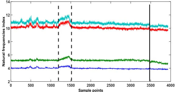
The Z24 bridge was a concrete highway structure in Switzerland connecting Koppigen and Utzenstorf, and in the late 1990s, before its demolishment procedure, it was used for SHM purposes under the ‘SIMCES’ project (Cross, 2012; Roeck, 2003). During a whole year of monitoring of the bridge, a series of sensor systems captured modal parameter measurements, as well as a family of environmental measurements such as air temperature, soil temperature, humidity, wind speed etc. The critical point in this benchmark project was the introduction of different types of real progressive damage scenarios towards the end of the monitoring year. For the purposes of this study, the four natural frequencies that were extracted over a period of year, including the period of structural failure of the bridge are used (see Figure 17).

Figure 17 Time history of frequencies (see online version for colours)

Sample points

0 500 1000 1500 2000 2500 3000 3500 4000

Natural frequencies index

2 4 6 8 10 12 14

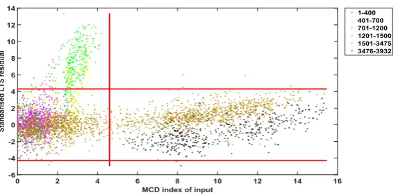
Figure 18 Plot of LTS residual versus MCD robust distance for regression between temperature and first natural frequency (linear LTS regression) (see online version for colours)

MCD index of input

0 2 4 6 8 10 12 14 16

Standarised LTS residual

-15 -10 -5 0 5 10 15 20 25 30 _1-400 401-700 701-1200 1201-1500 1501-3475 3476-3932

Source: Dervilis et al. (2014b, 2015)

Figure 19 Plot of LTS residual versus MCD robust distance for regression between temperature and second natural frequency (linear LTS regression) (see online version for colours)

MCD index of input

0 2 4 6 8 10 12 14 16

Standarised LTS residual

-25 -20 -15 -10 -5 0 5 10 15 20 25 _1-400 401-700 701-1200 1201-1500 1501-3475 3476-3932

Source: Dervilis et al. (2014b, 2015)

Figure 20 Plot of LTS residual versus MCD robust distance for regression between temperature and third natural frequency (linear LTS regression) (see online version for colours)

MCD index of input

0 2 4 6 8 10 12 14 16

Standarised LTS residual

-6 -4 -2 0 2 4 6 8 10 12 14 _1-400 401-700 701-1200 1201-1500 1501-3475 3476-3932

Figure 21 Plot of LTS residual versus MCD robust distance for regression between temperature and fourth natural frequency (linear LTS regression) (see online version for colours)

MCD index of input

0 2 4 6 8 10 12 14 16

Standarised LTS residual

-5 0 5

10 _1-400

401-700 701-1200 1201-1500 1501-3475 3476-3932

Source: Dervilis et al. (2014b, 2015)

As can be seen from in Figures 18–21, one can distinguish the different regions that were mentioned before. It can be noted the different characteristics between vertical outliers/region one (cold temperature influences), horizontal outliers (damage) and bad leverage points (damage). Environmental fluctuations due to temperature effects are different in nature than the damaged condition (region one or five) as they change the physical interpretation in the projection mapping. To make it even more clear, the fluctuation between observation 400–700 and between observations 1,200–1,500 when the temperature reaches the coldest values appear in the LTS results as vertical outliers. This was vital information as it showed that the nature of outliers between operational/environmental variations and damage have totally different characteristics (see an example in Figures 18–21). Table 2 explains the different regions as they appear in the graphs.

Table 2 Description of datasets as they appear in the figures

Observation Condition

1–400 Undamaged

401–700 Undamaged (with some cold temperature variations)

701–1,200 Undamaged (with some cold temperature variations)

1,201–1,500 Very cold temperature

1,501–3,475 Undamaged (with some hot temperature variations)

3,476–3,932 Damaged

5 Investigation of a nonlinear manifold

As a first step in investigating the performance of the LTS regression when a nonlinear system is present, simulated data were extracted via the following polynomial model with cubic terms:

3 0

( )

f x = +x x +x (8)

where {x} is a vector of data points coming from a Gaussian distribution with zero mean and unit standard deviation. The output vector was corrupted with a Gaussian noise vector of r.m.s. value 0.01.

Figure 22 Nonlinear simulated system (see online version for colours)

−3 −2 −1 0 1 2 3

−30

−20

−10 0 10 20 30

x observation

f(x) polynomial function

In Figure 22 can be seen the plot between input and output data. The training data points were chosen on purpose to be uniformly distributed between [–1, 1] in {x} where the function is fairly linear, with a small number of points added around +3 and –3.

Figure 23 Plot of LTS residual versus MCD robust distance for regression between x and f(x) (see online version for colours)

0 1 2 3 4 5 6

−200

−150

−100

−50 0 50 100 150 200

MCD index of input

Standarised LTS residual

As can be seen in Figure 23 the LTS algorithm for this clearly nonlinear relationship between input and output data wrongly classifies the edge points as bad leverage points, although they should be classified as good leverage points (as they belong to the normal condition of the polynomial function). As a result, the robust inclusive linear regression excludes the points at the edges and fits a good straight line to the centre dataset (see Figure 24).

Figure 24 Plot of the actual regression output line of robust measures (see online version for colours)

−3 −2 −1 0 1 2 3

−30

−20

−10 0 10 20 30

x observation

f(x) polynomial function

Training set LTS robust regression line

It is clear that the issue here is that the linear robust regression is not able to cope with nonlinear relationships. In this example LTS fails to characterise the edge points of the cubic polynomial as good leverage points in the projection map as these points are a natural regression continuation of the training dataset and not bad leverage points. In the next session an attempt to carry on with a possible nonlinear generalised model will be presented and not a unified framework technique for nonlinear cases as this is still an ongoing work and new theory is developing regarding the definitions of leverage points and outliers of nonlinear regression for SHM purposes.

6 Towards automatic nonlinear robust regression analysis

As shown in the previous part, the necessity of a nonlinear robust regression analysis is important after the identification and characterisation of the different outliers/leverage points in different families.

This analysis is possible if one changes the basis functions of the LTS algorithm by introducing a generalised linear model:

( )

( )

1 1 0for 1 and 1

i i i n j in

y =θu x + +… θ u x +θ i= …m j= …n (9)

7 A simple strategy for the Z24 bridge example

In this study a simple strategy is followed in order to allow the LTS technique to account for the vertical outliers at low temperatures (below zero) for the Z24 data shown before and classify them as good leverage points. As in the Z24 bridge, the environmental variations on the natural frequency are mainly caused due to low temperature values, one could introduce the following model:

( )

( )

1 1 2 2 0for 1

i i i

y =θu T +θ u T +θ i= …m (10)

where the basis functions work as bi-linear elements in the form of:

( )

( )

( )

( )

1 2

2 1

for 0 and 0 for 0 and

for 0 and 0 for 0 for 1

i i i i i

i i i i i

u T T T u T T

u T T T u T T

i m

= ≥ = ≤

= ≤ = ≥

= …

(11)

where T is the deck temperature. (In the case of the nonlinear polynomial example that was shown in previous section one could change the basis functions in order to account for the cubic terms.)

As can be seen from the results for three natural frequencies in Figures 25–28, the vertical outliers due to very low temperatures now appear as normal observations and the generalised bilinear LTS model performed very well in characterising the below zero measurements as normal/good leverage points. However, it can be noted that some few points that belong to very high temperatures (between observations 2,300–3,000) are not precisely classified as normal points which means that more basis functions in the generalised linear model might be needed in order to have a fully correct model that describes the Z24 bridge or it would be the case that some higher temperatures were included in the training data. Also, there is an indication of temporal increase of the mass of the bridge due to some trucks that were standing on the bridge during that period (Peeters and De Roeck, 2001).

Figure 25 Plot of LTS residual versus MCD robust distance for regression between temperature and first natural frequency (nonlinear LTS regression) (see online version for colours)

MCD index of input

0 1 2 3 4 5 6 7 8 9 10

Standarised LTS residual

Figure 26 Plot of LTS residual versus MCD robust distance for regression between temperature and second natural frequency (nonlinear LTS regression) (see online version for colours)

MCD index of input

0 1 2 3 4 5 6 7 8 9 10

Standarised LTS residual

-10 0 10 20 30 40

50 _1-400

401-700 701-1200 1201-1500 1501-3475 3476-3932

Figure 27 Plot of LTS residual versus MCD robust distance for regression between temperature and third natural frequency (nonlinear LTS regression) (see online version for colours)

MCD index of input

0 1 2 3 4 5 6 7 8 9 10

Standarised LTS residual

-10 0 10 20 30 40 50

60 _1-400

401-700 701-1200 1201-1500 1501-3475 3476-3932

Figure 28 Plot of LTS residual versus MCD robust distance for regression between temperature and fourth natural frequency (nonlinear LTS regression) (see online version for colours)

MCD index of input

0 1 2 3 4 5 6 7 8 9 10

Standarised LTS residual

-10 0 10 20 30 40

50 _1-400

8 Conclusions

In this paper, a review of robust outlier statistics for SHM applications is presented, focussed mainly on a high level estimation of the ‘masking effect’ of inclusive outliers, not only for determining the presence or absence of novelty – something that is of fundamental interest – but also to examine the normal condition set under the suspicion that it may already include multiple abnormalities due to EOVs (Dervilis et al., 2015).

The approach as proposed in this paper provides a first attempt to move LTS robust regression to a nonlinear perspective using the ideas of generalised linear regression models. After it was pointed out in previous work (Dervilis et al., 2015) that EOVs can manifest themselves differently (vertical outliers) in physical appearance compared to damage measurements, an effort to classify these vertical outliers as normal operational points or good leverage points is proposed.

Acknowledgements

The support of the UK Engineering and Physical Sciences Research Council (EPSRC) through grant reference number EP/J016942/1 and EP/K003836/2 is gratefully acknowledged.

References

Alampalli, S. (2000) ‘Effects of testing, analysis, damage, and environment on modal parameters’,

Mechanical Systems and Signal Processing, Vol. 14, No. 1, pp.63–74.

Antoniadou, I. (2013) Accounting for Nonstationarity in the Condition Monitoring of Wind Turbine

Gearboxes, PhD thesis.

Antoniadou, I. and Worden, K. (2014) ‘Use of a spatially adaptive thresholding method for the condition monitoring of a wind turbine gearbox’, EWSHM-7th European Workshop on

Structural Health Monitoring.

Attar, A.E., Khatoun, R. and Lemercier, M. (2013) ‘Diagnosing smartphone’s abnormal behavior through robust outlier detection methods’, Global Information Infrastructure Symposium, 2013, IEEE, pp.1–3.

Barnett, V. and Lewis, T. (1984) Outliers in Statistical Data, Vol. 1, John Wiley.

Cornwell, P., Farrar, C.R., Doebling, S.W. and Sohn, H. (1999) ‘Environmental variability of modal properties’, Experimental Techniques, Vol. 23, No. 6, pp.45–48.

Cross, E.J. (2012) On Structural Health Monitoring in Changing Environmental and Operational

Conditions, PhD thesis, University of Sheffield.

Cross, E.J., Koo, K.Y., Brownjohn, J.M.W. and Worden, K. (2013) ‘Long-term monitoring and data analysis of the Tamar bridge’, Mechanical Systems and Signal Processing, Vol. 35, No. 1, pp.16–34.

Cross, E.J., Worden, K. and Chen, Q. (2011) ‘Cointegration: a novel approach for the removal of environmental trends in structural health monitoring data’, Proceedings of the Royal Society

A: Mathematical, Physical and Engineering Science, Vol. 467, No. 2133, pp.2712–2732.

Dervilis, N., Choi, M., Taylor, S., Barthorpe, R., Park, G., Farrar, C. and Worden, K. (2014a) ‘On damage diagnosis for a wind turbine blade using pattern recognition’, Journal of Sound and

Dervilis, N., Cross, E.J., Barthorpe, R.J. and Worden, K. (2014b) ‘Robust methods of inclusive outlier analysis for structural health monitoring’, Journal of Sound and Vibration, Vol. 333, No. 20, pp.5181–5195.

Dervilis, N., Worden, K. and Cross, E. (2015) ‘On robust regression analysis as a means of exploring environmental and operational conditions for SHM data’, Journal of Sound and

Vibration, Vol. 347, pp.279–296.

Donoho, D.L. and Johnstone, J.M. (1994) ‘Ideal spatial adaptation by wavelet shrinkage’,

Biometrika, Vol. 81, No. 3, pp.425–455.

Farrar, C.R. and Worden, K. (2012) Structural Health Monitoring: A Machine Learning

Perspective, John Wiley & Sons.

Fritsch, V., Varoquaux, G., Thyreau, B., Poline, J-B. and Thirion, B. (2011) ‘Detecting outlying subjects in high-dimensional neuroimaging datasets with regularized minimum covariance determinant’, Medical Image Computing and Computer-Assisted Intervention – MICCAI 2011, Springer, pp.264–271.

Hawkins, D.M. (1980) Identification of Outliers, Vol. 11, Chapman and Hall, London.

Hubert, M. and Debruyne, M. (2010) ‘Minimum covariance determinant’, Wiley Interdisciplinary

Reviews: Computational Statistics, Vol. 2, No. 1, pp.36–43.

Hubert, M., Rousseeuw, P.J. and Van Aelst, S. (2008) ‘High-breakdown robust multivariate methods’, Statistical Science, pp.92–119.

Jackson, D.A. and Chen, Y. (2004) ‘Robust principal component analysis and outlier detection with ecological data’, Environmetrics, Vol. 15, No. 2, pp.129–139.

Khachiyan, L.G. (1996) ‘Rounding of polytopes in the real number model of computation’,

Mathematics of Operations Research, Vol. 21, No. 2, pp.307–320.

Khachiyan, L.G. and Todd, M.J. (1993) ‘On the complexity of approximating the maximal inscribed ellipsoid for a polytope’, Mathematical Programming, Vol. 61, No. 1, pp.137–159. Kumar, P. and Yildirim, E. (2005) ‘Minimum-volume enclosing ellipsoids and core sets’, Journal

of Optimization Theory and Applications, Vol. 126, No. 1, pp.1–21.

Leroy, A.M. and Rousseeuw, P.J. (1987) Robust Regression and outlier detection, Wiley Series in Probability and Mathematical Statistics, Wiley, New York.

Moshtagh, N. (2005) Minimum Volume Enclosing Ellipsoid, Convex Optimization.

Nurunnabi, A., Belton, D. and West, G. (2012) ‘Robust segmentation in laser scanning 3d point cloud data’, 2012 International Conference on Digital Image Computing Techniques and

Applications (DICTA), IEEE, pp.1–8.

Peeters, B. and De Roeck, G. (2001) ‘One-year monitoring of the z 24-bridge: environmental effects versus damage events’, Earthquake Engineering & Structural Dynamics, Vol. 30, No. 2, pp.149–171.

Peeters, B., Maeck, J. and De Roeck, G. (2001) ‘Vibration-based damage detection in civil engineering: excitation sources and temperature effects’, Smart Materials and Structures, Vol. 10, No. 3, p.518.

Roeck, G.D. (2003) ‘The state-of-the-art of damage detection by vibration monitoring: the SIMCES experience’, Journal of Structural Control, Vol. 10, No. 2, pp.127–134.

Rousseeuw, P. and Hubert, M. (2013) ‘High-breakdown estimators of multivariate location and scatter’, Robustness and Complex Data Structures, pp.49–66, Springer.

Rousseeuw, P.J. (1984) ‘Least median of squares regression’, Journal of the American Statistical

Association, Vol. 79, No. 388, pp.871–880.

Rousseeuw, P.J. and Van Driessen, K. (1999) ‘A fast algorithm for the minimum covariance determinant estimator’, Technometrics, Vol. 41, No. 3, pp.212–223.

Rousseeuw, P.J. and Van Driessen, K. (2006) ‘Computing LTS regression for large data sets’, Data

Mining and Knowledge Discovery, Vol. 12, No. 1, pp.29–45.

Schyns, M., Haesbroeck, G. and Critchley, F. (2010) ‘Relaxmcd: smooth optimisation for the minimum covariance determinant estimator’, Computational Statistics & Data Analysis, Vol. 54, No. 4, pp.843–857.

Sun, P. and Freund, R.M. (2004) ‘Computation of minimum-volume covering ellipsoids’,

Operations Research, pp.690–706.

Variyath, A.M. and Vattathoor, J. (2013) ‘Robust control charts for monitoring process mean of phase-i multivariate individual observations’, Journal of Quality and Reliability Engineering. Verboven, S. and Hubert, M. (2005) ‘Libra: a matlab library for robust analysis’, Chemometrics

and Intelligent Laboratory Systems, Vol. 75, No. 2, pp.127–136.