This is a repository copy of
Channel Equalization and Beamforming for Quaternion-Valued
Wireless Communication Systems
.
White Rose Research Online URL for this paper:
http://eprints.whiterose.ac.uk/107914/
Version: Accepted Version
Article:
Liu, W. orcid.org/0000-0003-2968-2888 (2016) Channel Equalization and Beamforming for
Quaternion-Valued Wireless Communication Systems. Journal of the Franklin Institute.
ISSN 0016-0032
https://doi.org/10.1016/j.jfranklin.2016.10.043
Article available under the terms of the CC-BY-NC-ND licence
(https://creativecommons.org/licenses/by-nc-nd/4.0/)
[email protected] https://eprints.whiterose.ac.uk/ Reuse
This article is distributed under the terms of the Creative Commons Attribution-NonCommercial-NoDerivs (CC BY-NC-ND) licence. This licence only allows you to download this work and share it with others as long as you credit the authors, but you can’t change the article in any way or use it commercially. More
information and the full terms of the licence here: https://creativecommons.org/licenses/
Takedown
If you consider content in White Rose Research Online to be in breach of UK law, please notify us by
Channel Equalization and Beamforming for Quaternion-Valued Wireless
Communication Systems
Wei Liua
aCommunication Research Group, Department of Electronic and Electrical Engineering, University of Sheffield
Sheffield, S1 4ET, United Kingdom, Tel.: +44-114-2225813; fax: +44-114-2225834
Abstract
Quaternion-valued wireless communication systems have been studied in the past. Although progress has been made in this promising area, a crucial missing link is lack of effective and efficient quaternion-valued signal processing algorithms for channel equalization and beamforming. With most recent developments in quaternion-valued signal processing, in this work, we fill the gap to solve the problem by studying two quaternion-valued adaptive algorithms: one is the reference signal based quaternion-valued least mean square (QLMS) algorithm and the other one is the quaternion-valued constant modulus algorithm (QCMA). The quaternion-valued Wiener solution for possible block-based calculation is also derived. Simulation results are provided to show the working of the system.
Keywords: Polarisation diversity, four-dimensional modulation, quaternion valued signal processing, channel equalization, beamforming, constant modulus, least mean square.
1. Introduction
Increasing the capacity of a wireless communication system has always been a focus of the wireless communi-cations research community. It is well-known that polarisation diversity can be exploited to mitigate the multipath effect to maintain a reliable communication link with an acceptable quality of service (QoS), where a pair of anten-nas with orthogonal polaristion directions is employed at both the transmitter and the receiver sides. However, the traditional diversity scheme aims to achieve a single reliable channel link between the transmitter and the receiver, while the same information is transmitted at the same frequency but with different polarisations, i.e. two channels. This is not an effective use of the precious spectrum resources as the two channels could be used to transmit different data streams simultaneously. For example, we can design a four-dimensional (4-D) modulation scheme across the two polarisation diversity channels using a quaternion-valued representation, as proposed in [1]. An earlier version of quaternion-valued 4-D modulation scheme based on two different frequencies was proposed in [2]. However, due to the change of polarisation of the transmitted radio frequency signals during the complicated propagation process including multipath, reflection, refraction, etc, interference will be caused to each other at the two differently polarised receiving antennas. To solve the problem, efficient signal processing methods and algorithms for channel equalization and interference suppression/beamforming are needed for practical implementation of the proposed 4-D modulation scheme.
Recently, quaternion-valued signal processing has been introduced and studied in details to solve problems related to three or four-dimensional signals [3], such as vector-sensor array signal processing [4, 5, 6, 7, 8, 9], and wind profile prediction [10]. With most recent developments in this area, especially the derivation of quaternion-valued gradient operators and the quaternion-valued least mean square (QLMS) algorithm [11, 10, 12], we are now ready to effectively solve the 4-D equalisation and interference suppression/beamforming problem associated with the proposed 4-D mod-ulation scheme. Now the dual-channel effect on the transmitted signal can be modeled by a quaternion-valued infinite impulse response (IIR) or finite impulse response (FIR) filter. At the receiver side, for channel equalisation, we can
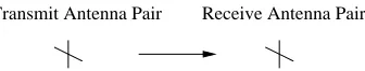
Transmit Antenna Pair Receive Antenna Pair
Figure 1: Wireless communication employing polarisation diversity, where both the transmitter and the receiver sides are equipped with a pair of antennas with different polarisation directions.
employ a quaternion-valued adaptive algorithm to recover the original 4-D signal, which inherently also performs an interference suppression operation to separate the original two 2-D signals. Moreover, multiple antenna pairs can be employed at the receiver side to perform the traditional beamforming task to suppress other interfering signals.
In particular, two representative quaternion-valued equalisation/beamforming algorithms will be derived: the first one is the quaternion-valued Wiener filter as a follow-up to the previously derived QLMS algorithm for reference signal based equalisation/beamforming, and the second one is the quaternion-valued constant modulus algorithm (QCMA) for blind equalisation/beamforming. Compared to the summary contribution in [13], in addition to the detailed analytical modeling steps, the main difference is the GCMA algorithm and the related simulations. Although quaternion-valued wireless communication employing multiple antennas has been studied before, such as the design of orthogonal space-time-polarization block code in [14], to our best knowledge, it is the first time to study the quaternion-valued equalization and interference suppression/beamforming problem in this context. Moreover, the dual-polarised antenna pair or an array of them has a similar structure to the well-studied vector sensors or sensor arrays [15, 16, 17, 18], where they are used mainly for traditional array signal processing applications. Although the recently developed quaternion-valued array signal processing algorithms based on such traditional array applications employed a quaternion-valued array model [4, 5, 6], the desired signals are still traditional complex-valued signals, instead of quaternion-valued communication signals.
In the following, the 4-D modulation scheme based on two orthogonally polarised antennas will be introduced in Sec. 2 and the required quaternion-valued equalisation and inter-channel interference suppression solution and their extension to multiple dual-polarised antennas are presented in Sec. 3. Simulation results are provided in Sec. 4, followed by conclusions in Sec. 5.
2. Quaternion-Valued 4-D Modulation
In traditional polarisation diversity scheme, as shown in Fig. 1, each side is equipped with two antennas with orthogonal polarisation directions and the signal being transmitted is two-dimensional, i.e. complex-valued with one real part and one imaginary part. In the quaternion-valued modulation scheme, the signal is modulated across the two antennas to generate a 4-D modulated signal. Such a signal can be conveniently represented mathematically by a quaternion [19, 20]. A quaternion is a hypercomplex number defined as
q=q0+iq1+jq2+kq3, (1)
where q0is the real part of the quaternion, and q1, q2and q3 are the three imaginary components with their corre-sponding imaginary units i, j and k, respectively. The conjugate of a quaternion, denoted by q∗, is defined as
q∗=q0−iq1−jq2−kq3. (2)
i, j and k satisfy the following conditions
ii= j j=kk=−1, (3)
i j=−ji=k,jk=−k j=i,ki=−ik= j. (4)
As a result, quaternionic multiplications are noncommutative.
e
y
s
r
q
s
− +]
n
[
]
n
]
[n
n
]
[
[ n
]
n
[
t c r a [image:4.595.193.406.111.176.2]f n ]
[
[ ]
w
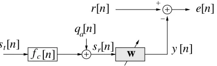
Figure 2: Channel model and the reference signal based equalizer for quaternion-valued signals.
3. Quaternion-Valued Equalization and Interference Suppression/Beamforming
3.1. Channel model
The signal transmitted by the two antennas will go through the channel with all kinds of effects and arrive at the receiver side, where the two antennas with orthogonal polarisation directions (Note that orthogonal polarisation may not give the best performance for a specific scenario) will pick up the two signals. Again the four components of the received signal can be represented by another quaternion. We use st[n] and sr[n] to represent the transmitted and received 4-D quaternion-valued signals, respectively. Then the channel effect can be modeled by a filter with quaternion-valued impulse response fc[n], i.e.
sr[n]=st[n]∗ fc[n]+qa[n], (5)
where qa[n] is the quaternion-valued additive noise, as shown in Fig. 2.
3.2. Reference signal based approach
To recover st[n] from sr[n] or estimate the channel, as in the 2-D case (complex-valued), we can design a quaternion-valued equalizer. One choice is a reference signal based equalizer, among many others corresponding to the complex-valued case. Now assume we have a reference signal r[n] available. Then we can employ the standard adaptive filtering structure shown in the second half of Fig. 2 and update the equalizer coefficient vector w with a length of L by minimising the mean square value of the error signal e[n] [10, 12].
The cost function is given by
J[n]=e[n]e∗[n], (6)
where
e[n]=r[n]−y[n]=r[n]−wTsr[n]. (7)
with w being the equalizer coefficient vector and sr[n] holding the corresponding received signal samples from sr[n]
w = [w0,w1,· · ·,wL−1]T
sr[n] = [sr[n],sr[n−1],· · ·,sr[n−L+1]]T . (8)
For a general quaternion-valued function f (q) of a quaternion q, the gradient of f with respect to q is defined as [10, 12]
∂f
∂q := 1 4
∂f
∂q0
− ∂f
∂q1 i− ∂f
∂q2 j− ∂f
∂q3 k
!
, (9)
∂f
∂q∗ := 1 4
∂f
∂q0 +
∂f
∂q1 i+ ∂f
∂q2 j+k∂f
∂q3 k
!
, (10)
Following the derivations in [10, 12], we have the gradient of J[n] with respect to the coefficient vector as follows
∇wJ[n]=−
1 2sr[n]e
∗
which leads to the following update equation for the coefficient vector with a step size ofµ, i.e. the QLMS algorithm:
w[n+1] = w[n]−µ(∇wJ[n])∗ (12)
= w[n]+µ(e[n]s∗r[n]). (13)
For a solution equivalent to the classic Wiener filter in the complex-valued case, based on the instantaneous gradient result of (11), the optimum solution woptshould satisfy
E{−1
2sr[n]e ∗[n]}
=0, (14)
i.e.
E{sr[n]e∗[n]} = E{sr[n]r∗[n]−sr[n]sHr[n]w ∗ opt}
= p−Rsrw ∗
opt =0, (15)
where the cross-correlation vector p=E{sr[n]r∗[n]}and the covariance matrix Rsr=E{sr[n]s H
r[n]}. Then we have
Rsrw ∗
opt=p ⇒ w ∗ opt=R
−1
srp. (16)
We can use the above equation to obtain the optimum weight vector directly.
Now consider the multiplication of two quaternions a and b with c=ab. They are expressed as
a = a0+ia1+ja2+ka3 b = b0+ib1+jb2+kb3
c = c0+ic1+jc2+kc3 (17)
where the subscripts indicate the corresponding components of the quaternion. Then we have
c0 = b0a0−b1a1−b2a2−b3a3
c1 = b0a1+b1a0−b2a3+b3a2 c2 = b0a2+b1a3+b2a0−b3a1
c3 = b0a3−b1a2+b2a1+b3a0 (18)
Using this result, we can obtain the solution to (16) using real-valued matrix operations. First we define the following two vectors
ˆ
wopt = [R(w∗opt,0),−I(w ∗
opt,0),−J(w ∗
opt,0),−K(w ∗ opt,0),
· · · ,R(w∗opt,L−1),−I(w∗opt,L−1),−J(w∗opt,L−1),−K(w∗opt,L−1)]|T
ˆp = [R(p)T,I(p)T,J(p)T,K(p)T]T , (19)
where wopt,l, l =0,· · ·,L−1 is the l-th element of the optimum weight vector wopt, R(·), I(·), J(·), and K(·) are the operation of taking the real and three imaginary components of the quaternion inside the brackets, respectively. We also define
ˆ
Rsr=[ ˆRsr,0;· · · ; ˆRsr,L−1], (20) with
ˆ
Rsr,l=
R(rl) −I(rl) −J(rl) −K(rl)
I(rl) R(rl) −K(rl) +J(rl)
J(rl) K(rl) R(rl) −I(rl)
K(rl) −J(rl) I(rl) R(rl)
(21)
Then, according to (16), we have the following relationship
ˆ
Rsrwˆopt= ˆp, (22)
where all the matrix and vectors involved are real-valued. Then ˆwoptis obtained by
ˆ
wopt=Rˆ −1
sr ˆp. (23)
From ˆwopt, we can then easily deduce wopt.
3.3. Constant modulus based approach
When a reference signal is not available, it is still possible to perform equalisation and interference suppres-sion/beamforming by employing other properties of the signals. An algorithm designed to work without knowledge of the transmitted signals falls into the category of blind equalisation and beamforming approaches [21, 22, 23]. One representative blind equalisation algorithm in traditional communication systems is the constant modulus algorithm (CMA) [24, 25, 26, 27, 28, 29].
There are many variations to this algorithm and the basic form is based on minimizing the following cost function
JCM =14E{(|y[n]|2−γ)2}, (24)
where y[n] is the output of the equalizer andγis the dispersion constant, defined byγ= E{sk}4
E{sk}2 with skbeing symbols of the modulation scheme.
For our quaternion-valued 4-D wireless communication system, we can develop a similar quaternion-valued CMA (QCMA) for blind equalization and beamforming. Taking the gradient of JCM with respect to the quaternion-valued coefficient vector w, and using the third chain rule of the restricted HR gradient operation given in [12] as the inter-mediate function is real-valued, we have
∇wJCM = 12E{(y[n]·y∗[n]−γ)∂(y[n]·y
∗[n]−γ)
∂w }
= 1
2E{(y[n]·y
∗[n]−γ)∂(y[n]·y ∗[n])
∂w }
= 12E{(y[n]·y∗[n]−γ)∂(w
Ts
r[n]sHr[n]w∗)
∂w }
(25)
Using the result of [10], we have
∂(wTsr[n]sHr[n]w∗)
∂w =
1 2sr[n]y
∗[n] (26)
Then we have
∇wJCM = 14E{(y[n]·y∗[n]−γ)sr[n]y∗[n]} (27)
Using the instantaneous gradient ˆ∇wJCMto replace∇wJCM, we then obtain the final update equation for our quaternion-valued constant modulus algorithm
w[n+1] = w[n]−µ(∇wJCM)∗ (28)
= w[n]−µ(|y[n]|2−γ)y[n]s∗r[n], (29)
where the constant1
Transmit Antenna Pair
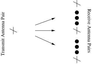
[image:7.595.219.378.112.222.2]Receive Antenna Pairs
Figure 3: Multiple antenna pairs at the receiver side, where each pair is composed of two differently polarised antennas.
Transmit Antenna Pairs
[image:7.595.218.379.254.370.2]Receive Antenna Pairs
Figure 4: A MIMO system with multiple antenna pairs at both the transmitter and the receiver sides, where each pair is composed of two differently polarised antennas.
3.4. Extension to multiple antennas and MIMO systems
We can extend this design to multiple antenna pairs for beamforming to suppress other quaternion-valued interfer-ing signals, as shown in Fig. 3, or Fig. 4 for a general multiple-input-multiple-output (MIMO) system. The channel model for an M×N system is shown in Fig. 5, where st,m[n], m =0,1,· · ·,M−1 is the transmitted signal, while
sr,l[n], l=0,1,· · ·,N−1 is the received signal. qa,l[n], l=0,1,· · ·,N−1 is the added channel noise and fm,l[n] is the quaternion-valued channel impulse response between the m-th transmit antenna pair and the l-th receive antenna pair.
Mathematically, we have
sr[n]=AT ·st[n]+qa[n], (30)
where
A =
f0,0[n] f0,1[n] . . . f0,N−1(t) f1,0[n] f1,1[n] . . . f1,N−1(t)
..
. ... . .. ...
fM−1,0[n] fM−1,1[n] . . . fM−1,N−1[n]
,
st[n] = [st,0[n],st,1[n],· · ·,st,M−1]T
sr[n] = [sr,0[n],sr,1[n],· · ·,sr,N−1]T
qa[n] = [qa,0[n],qa,1[n],· · ·,qa,N−1]T (31)
Applying an L×1 weight vector wm,l=[wm,l,0,wm,l,1,· · ·,wm,l,L−1]T, m=0,1,· · ·,M−1, l=0,1,· · ·,N−1, to
the received signal sr,l[n] and then combining the N corresponding outputs together, we obtain one of the estimated signals ym[n], i.e.
[n]
q
a,0
s
r,N−1[n]
[n]
s
t,M−1s
t,0a,N−1
q
[n]
[n]
[n]
f
M−1,0[n]
f
[n]
M−1,N−1
[n]
f
0,0
f
0,N−1 [image:8.595.192.403.109.214.2]s
r,0[n]
Figure 5: Channel model for a quaternion-valued MIMO system.
1000 2000 3000 4000 5000 6000 7000 8000 9000 10000
−14 −12 −10 −8 −6 −4 −2 0 2
Iterations
Ensemble Mean Square Error [dB]
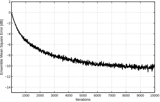
Figure 6: Learning curve of the quaternion-valued equalizer using the QLMS algorithm.
where
wm = [wTm,0,w
T
m,1,· · ·,w
T m,N−1]
T
ˆsr[n] = [sTr,0[n],s
T
r,1[n],· · ·,s
T r,N−1[n]]
T
sr,l[n] = [sr,l[n],sr,l[n−1],· · ·,sr,,l[n−L+1]]T . (33)
The optimum weight vector for wmcan be obtained using either the QLMS algorithm or the QCMA introduced before so that ym[n] becomes a good estimate of one of the transmitted signals.
4. Simulation Results
In the following, we give three sets of simulation results. The first two are for the QLMS algorithm and the third one for the QCMA.
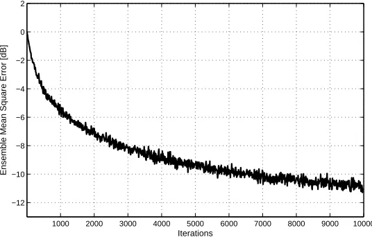
The first set of simulations is based on the structure in Fig. 2 and it is a reference-signal based channel equalization problem. The signal transmitted is 16-Q2AM modulated and the SNR at the receiver side is 20 dB with quaternion-valued Gaussian noise. The channel impulse response fc[n] is a 4-tap quaternion-valued FIR filter with a Gaussian-distributed coefficients value, which is generated randomly for each run. The equalizer filter has a length of 15. The learning curve based on averaging 200 simulation runs using the QLMS algorithm is shown in Fig. 6 with a step size
[image:8.595.163.434.248.421.2]−20 −10 0 10 20 −20 −10 0 10 20 Real part i component
−20 −10 0 10 20 −20 −10 0 10 20 j component k component
−2 −1 0 1 2 −2 −1 0 1 2 Real part i component
[image:9.595.154.444.112.347.2]−2 −1 0 1 2 −2 −1 0 1 2 j component k component
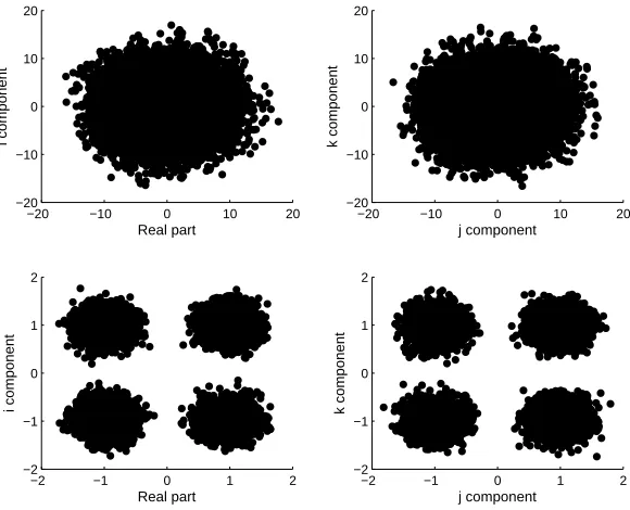
Figure 7: Scatter plots before (two upper sub-figures) and after (two lower sub-figures) equalization using the QLMS algorithm.
However, if we focus on one specific channel response, such as the one given below
−1.1696 0.4989 1.0571 0.4911
−0.1135 −0.3639 −0.3791 0.8653 0.0958 −0.2515 1.4957 0.1552
−0.9583 −0.6047 0.5183 −0.8966
, (34)
where each column gives the four components of the quaternion-valued coefficient of fc[n], and use the same value ofµ =0.000012, we will be able to achieve a zero BER result, as shown by the scatter plots of constellation before and after equalization in Fig. 7. Since we can not show the 4-D scatter plot directly, we have split it into two 2-D plots in Fig. 7, where the upper row is for the scatter plots before equalization, and the lower row for the plots after equalization. We can clearly see that the equalization operation has been successful.
In the second set of simulations, we consider a 2×2 MIMO array and the two transmitted quaternion-valued signals have the same normalized power, with an SNR of 20 dB at the receiver side. All the other parameters are the same as the first one, except that now the step size has been changed toµ=0.0000006. Fig. 8 shows the result, again a reasonable performance with such a fixed non-optimum step size.
Moreover, we have used the MATLAB function ‘tic’ and ‘toc’ to calculate the running time for the two scenarios. Based on a Windows 7 computer with Intel Core i5-2467M CPU (1.60GHz) and 4GB memory, it took about 4.9 seconds for each run of the first scenario and 10.6 seconds for each run of the second scenario. This time is dependent on the stepsize adopted for the algorithm. A larger stepsize will significantly reduce the time required for convergence. The reason for our current step size value (which is quite small) is to make sure the algorithm will converge for all channel realizations in the simulation. In practice, this step size could be normalized according to the received signal powers to give a much faster convergence rate, in a similar way to the normalized LMS algorithm in literature for complex-valued signals [30, 23].
Now we consider an example for the QCMA. A well-known problem with constant modulus based algorithm is that it may converge to local minima depending on its initial values. We find that it is very difficult to initialize the algorithm properly to perform both the equalization and beamforming tasks simultaneously based on the general MIMO structure. So here we only show a case for blind equalization using the QCMA. The setting is the same as the first set of simulations. Since we are using the 16-Q2AM modulation scheme, we have chosenγ=4. The stepsize is
1000 2000 3000 4000 5000 6000 7000 8000 9000 10000 −12
−10 −8 −6 −4 −2 0 2
Iterations
[image:10.595.163.431.114.285.2]Ensemble Mean Square Error [dB]
Figure 8: Learning curve of the quaternion-valued equalizer/MIMO beamformer using the QLMS algorithm.
1000 2000 3000 4000 5000 6000 7000 8000 9000 10000
−7 −6 −5 −4 −3 −2 −1 0 1 2
Iterations
[image:10.595.163.429.322.494.2]Ensemble Instantaneous Cost Function [dB]
Figure 9: Learning curve of the quaternion-valued constant modulus algorithm.
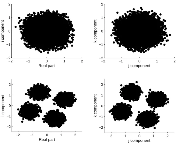
The learn curve in terms of the instantaneous cost function 14(|y[n]|2−4)2 averaged over 200 runs is shown in Fig. 9, where we can observe that the approximately constant modulus status has been reached. The scatter plots of constellation before and after equalization for the specific channel realization in (34) are shown in Fig. 10, which clearly demonstrate that the equalization operation has been successful. One note is the phase shift in the plot, which is normal as the blind equalization algorithm we employed here is ambiguous to an arbitrary phase shift.
5. Conclusions
−2 −1 0 1 2 −2
−1 0 1 2
Real part
i component
−2 −1 0 1 2 −2
−1 0 1 2
j component
k component
−2 −1 0 1 2 −2
−1 0 1 2
Real part
i component
−2 −1 0 1 2 −2
−1 0 1 2
j component
[image:11.595.153.442.110.345.2]k component
Figure 10: Scatter plots before (two upper sub-figures) and after (two lower sub-figures) equalization using the quaternion-valued constant modulus algorithm.
and multiple-input-multiple-output cases and such a 4-D modulation scheme can therefore be considered as a viable approach for future wireless communication systems.
References
[1] O. M. Isaeva and V. A. Sarytchev, “Quaternion presentations polarization state,” in Proc. 2nd IEEE Topical Symposium of Combined
Optical-Microwave Earth and Atmosphere Sensing, Atlanta, US, April 1995, pp. 195–196.
[2] L. H. Zetterberg and H. Br¨andstr¨om, “Codes for combined phase and amplitude modulated signals in a four-dimensional space,” IEEE
Transactions on Communications, vol. COM-25, no. 29, pp. 943–950, September 1977.
[3] N. Le Bihan and J. Mars, “Singular value decomposition of quaternion matrices: a new tool for vector-sensor signal processing,” Signal
Processing, vol. 84, no. 7, pp. 1177–1199, 2004.
[4] S. Miron, N. Le Bihan, and J. I. Mars, “Quaternion-MUSIC for vector-sensor array processing,” IEEE Transactions on Signal Processing, vol. 54, no. 4, pp. 1218–1229, April 2006.
[5] X. F. Gong, Z. W. Liu, and Y. G. Xu, “Direction finding via biquaternion matrix diagonalization with vector-sensors,” Signal Processing, vol. 91, no. 4, pp. 821–831, 2011.
[6] J. W. Tao and W. X. Chang, “A novel combined beamformer based on hypercomplex processes,” IEEE Transactions on Aerospace and
Electronic Systems, vol. 49, no. 2, pp. 1276–1289, 2013.
[7] X. R. Zhang, W. Liu, Y. G. Xu, and Z. W. Liu, “Quaternion-valued robust adaptive beamformer for electromagnetic vector-sensor arrays with worst-case constraint,” Signal Processing, vol. 104, pp. 274–283, November 2014.
[8] M. B. Hawes and W. Liu, “Design of fixed beamformers based on vector-sensor arrays,” International Journal of Antennas and Propagation, 2015.
[9] M. D. Jiang, W. Liu, and Y. Li, “Adaptive beamforming for vector-sensor arrays based on reweighted zero-attracting quaternion-valued LMS algorithm,” in IEEE Transactions on Circuits and Systems II: Express Briefs, vol. 63, Issue 3, pp. 274-278, March 2016.
[10] M. D. Jiang, W. Liu, and Y. Li, “A general quaternion-valued gradient operator and its applications to computational fluid dynamics and adaptive beamforming,” in Proc. of the International Conference on Digital Signal Processing, Hong Kong, August 2014.
[11] D. P. Mandic, C. Jahanchahi, C. C. Took, “A quaternion gradient operator and its applications,” IEEE Signal Processing Letters, vol. 18, pp.47-50, January 2011.
[12] M. D. Jiang, Y. Li, and W. Liu, “Properties of a General Quaternion-Valued Gradient Operator and Its Application to Signal Processing,”
Frontiers of Information Technology & Electronic Engineering, vol. 17, pp. 83-95, February 2016.
[13] W. Liu, “Antenna array signal processing for a quaternion-valued wireless communication system,” in Proc. the Benjamin Franklin
Sympo-sium on Microwave and Antenna Sub-systems (BenMAS), Philadelphia, US, September 2014.
[15] R. T. Compton, “The tripole antenna: An adaptive array with full polarization flexibility,” IEEE Transactions on Antennas and Propagation, vol. 29, no. 6, pp. 944–952, November 1981.
[16] A. Nehorai, K. C. Ho, and B. T. G. Tan, “Minimum-noise-variance beamformer with an electromagnetic vector sensor,” IEEE Transactions
on Signal Processing, vol. 47, no. 3, pp. 601–618, March 1999.
[17] M. D. Zoltowski and K. T. Wong, “ESPRIT-based 2D direction finding with a sparse uniform array of electromagnetic vector-sensors,” IEEE
Transactions on Signal Processing, vol. 48, pp. 2205–2210, August 2000.
[18] X. R. Zhang, Z. W. Liu, Y. G. Xu, and W. Liu, “Adaptive tensorial beamformer based on electromagnetic vector-sensor arrays with coherent interferences,” Multidimensional Systems and Signal Processing, vol. 26, issue 3, pp. 803-821, July 2015.
[19] W. R. Hamilton, Elements of Quaternions, Longmans, Green, & co., 1866.
[20] I. Kantor, A. S. Solodovnikov, and A. Shenitzer, Hypercomplex Numbers: an Elementary Introduction to Algebras, Springer Verlag, New York, 1989.
[21] Z. Ding and Y. Li, Blind Equalisation and Identification, Signal Processing and Communications. CRC, New York, 2001. [22] H. L. Van Trees, Optimum Array Processing, Part IV of Detection, Estimation, and Modulation Theory, Wiley, New York, 2002. [23] W. Liu and S. Weiss, Wideband Beamforming: Concepts and Techniques, John Wiley & Sons, Chichester, UK, 2010.
[24] R. Gooch and J. Lundell, “CM array: an adaptive beamformer for constant modulus signals,” in Proc. IEEE International Conference on
Acoustics, Speech, and Signal Processing, New York, NY, 1986, pp. 2523–2526.
[25] H. Krim and M. Viberg, “Two decades of array signal processing research: the parametric approach,” IEEE Signal Processing Magazine, vol. 13, no. 4, pp. 67–94, July 1996.
[26] L. C. Godara, “Application of antenna arrays to mobile communications, part ii: Beam-forming and direction-of-arrival estimation,”
Pro-ceedings of the IEEE, vol. 85, no. 8, pp. 1195–1245, August 1997.
[27] C. R. Johnson, P. Schniter, T. J. Endres, J. D. Behm, D. R. Brown, and R. A. Casas, “Blind equalization using the constant modulus criterion: A review,” Proceedings of the IEEE, vol. 86, no. 10, pp. 1927–1950, October 1998.
[28] S. Chen, A. Wolfgang, and L. Hanzo, “Constant modulus algorithm aided soft decision directed scheme for blind space-time equalisation of SIMO channels,” Signal Processing, vol. 87, pp. 2587–2599, November 2007.
[29] L. Zhang, W. Liu, and R. J. Langley, “A class of constant modulus algorithms for uniform linear arrays with a conjugate symmetric constraint,”
Signal Processing, vol. 90, pp. 2760–2765, September 2010.