This is a repository copy of
Accelerating the computation of critical eigenvalues with
parallel computing techniques
.
White Rose Research Online URL for this paper:
http://eprints.whiterose.ac.uk/105995/
Version: Accepted Version
Proceedings Paper:
Aristidou, P orcid.org/0000-0003-4429-0225 and Hug, G (2016) Accelerating the
computation of critical eigenvalues with parallel computing techniques. In: Power Systems
Computation Conference (PSCC), 2016. Genova, Italy, 20-24 Jun 2016, 2016 Power
Systems Computation Conference (PSCC). Power Systems Computation Conference .
ISBN 978-88-941051-2-4
https://doi.org/10.1109/PSCC.2016.7540976
© 2016 IEEE. Personal use of this material is permitted. Permission from IEEE must be
obtained for all other users, including reprinting/ republishing this material for advertising or
promotional purposes, creating new collective works for resale or redistribution to servers
or lists, or reuse of any copyrighted components of this work in other works.
[email protected] https://eprints.whiterose.ac.uk/
Reuse
Unless indicated otherwise, fulltext items are protected by copyright with all rights reserved. The copyright exception in section 29 of the Copyright, Designs and Patents Act 1988 allows the making of a single copy solely for the purpose of non-commercial research or private study within the limits of fair dealing. The publisher or other rights-holder may allow further reproduction and re-use of this version - refer to the White Rose Research Online record for this item. Where records identify the publisher as the copyright holder, users can verify any specific terms of use on the publisher’s website.
Takedown
If you consider content in White Rose Research Online to be in breach of UK law, please notify us by
Accelerating the Computation of Critical
Eigenvalues with Parallel Computing Techniques
Petros Aristidou
Power System Laboratory, ETH Zürich, Zürich, Switzerland
Email: [email protected]
Gabriela Hug
Power System Laboratory, ETH Zürich, Zürich, Switzerland
Email: [email protected]
Abstract—Eigenanalysis of power systems is frequently used to study the effect and tune the response of existing controllers, or to guide the design of new controllers. However, recent developments in the area lead to the necessity of studying larger power system models, resulting from the interconnection of transmission networks or the joint consideration of transmission and distribution networks. Moreover, these models include new types of controls, mainly based on power electronic interfaces, which are expected to provide significant support in the future. The consequence is that the size and complexity of these models challenge the computational efficiency of existing eigenanalysis methods. In this paper, a procedure is proposed that uses domain decomposition and parallel computing methods, to accelerate the computation of eigenvalues in a selected region of the complex plane with iterative eigenanalysis methods. The proposed algorithm is validated on a small transmission system and its performance is assessed on a large-scale, combined transmission and distribution system.
Index Terms—eigenanalysis, domain decomposition, parallel computing, OpenMP, implicitly restarted Arnoldi
I. INTRODUCTION
Small-signal analysis allows extracting information on the stability and dynamic characteristics of power systems, and is essential for the design, coordination, and integration of controllers [1]. Classical problems tackled by eigenanalysis are the configuration of Power System Stabilizers (PSSs), Automatic Voltage Regulators (AVRs), and speed governors [2]. Other applications involve the analysis of controls and sta-bilizers for FACTS-based devices, and studying the dynamic performance of Wind-Turbine (WT) generators, PhotoVoltaic (PV) generators, HVDC converters, etc. [1]. The latter are expected to play a significant role in the desired transition to a sustainable electric power system.
The eigenanalysis can be performed with full space methods such as QR and QZ [3], which can compute all the eigenvalues. These methods are computationally and memory intensive and can be efficiently used for systems up to few thousand variables. For larger systems, iterative methods such as the Implicitly Restarted Arnoldi Method (IRAM) [4], the Jacobi-Davidson QZ (JDQZ) [4], or the inverse power iteration [5], are frequently used. These methods compute eigenvalues only in a selected region of the complex plane and can handle systems with several thousand variables.
Recent developments in power systems require the analysis of increasingly larger models. These can involve large-scale
interconnected systems, such as the European Interconnected system, or combined transmission and distribution systems, in order to study the contribution of active distribution network controls and Distributed Generators (DGs) to the system dy-namics. The size and complexity of these models challenge the computational efficiency even of iterative eigenanalysis meth-ods and can decrease the productivity of engineers (increased time spent on waiting for the calculations and getting results). Various techniques have been proposed to exploit the structure and sparsity of the matrices to accelerate the computations [5], [6], [7]. While other techniques employ parallelization for the computation of eigenvalues in different areas of the complex plane [8], [9] or parallelize the computation of each pair of eigenvalues [10], [11], [12].
In this paper, a new parallel procedure is proposed to accelerate the solution of linear systems required by iterative eigenanalysis methods. First, a topological-based decompo-sition of the power system is performed, revealing a non-overlapping, star-shaped partitioning, similar to [13]. Next, the Differential-Algebraic Equations (DAEs) describing the power system are projected onto the sub-domains, formulating the corresponding sub-problems. The latter are linearized, providing anequivalent, decomposed description of the system which is needed for eigenanalysis. Thus, the requested solution of the linear system is computed implicitly, using parallel computing techniques, and without the need to eliminate the algebraic states. Finally, a Schur-complement approach is used to treat the interface variables between the sub-domains, thus ensuring the accuracy of the decomposed solution.
The proposed procedure exploits the sparsity of the power system matrices and accelerates the solution by parallelizing the factorization and solution of the sub-systems. In addition, the decomposition of the system allows to skip some unnec-essary computations, without affecting the solution accuracy. The proposed Decomposed Parallel Solver (DPS) is imple-mented with the use of shared-memory parallel computing techniques through the OpenMP Application Programming Interface (API), targeting common, inexpensive multi-core machines.
used to validate its accuracy, and also a large-scale, combined transmission and distribution system model (137186DAEs) to assess its performance on a multi-core desktop computer.
The paper is organized as follows. In Section II, the power system dynamic model and the eigenvalue problem are re-viewed. In Section III, the proposed domain decomposition-based solution is presented. In Section IV, the implementation specifics are detailed. Simulation results are reported in Sec-tion V and followed by closing remarks in SecSec-tion VI.
II. POWERSYSTEMMODEL ANDEIGENVALUEPROBLEM A complex power system is usually modeled with a set of DAEs [2], as follows:
0 = Ψ(x,V) (1a) Γx˙ = Φ(x,V) (1b)
whereV is the vector of voltages at the buses of the network and x is the state vector containing the remaining (except voltages) differential and algebraic variables of the system. Furthermore, Γ is a diagonal matrix with:
(Γ)ℓℓ=
(
0 ifℓ-th equation is algebraic
1 ifℓ-th equation is differential (2) The algebraic Eqs. (1a) describe the network and can be rewritten as:
0=DV −I=Ψ(x,V) (3)
where D includes the real and imaginary parts of the bus admittance matrix and I is a sub-vector of x containing the bus currents.
Equation (1b) describes the remaining DAEs of the system including the dynamics of generating units, their controls, dynamic loads, and other devices. Together these equations form a complete mathematical model of the system.
For the purpose of small-signal stability analysis, the DAE model (1) is linearized around a given system operating point [1]. This yields the following linearized system:
0 0
0 Γ
| {z }
E
0
∆ ˙x
=
Ψ
V Ψx
ΦV Φx
| {z }
J
∆V
∆x
(4)
whereJ is the Jacobian matrix of (1) in descriptor form [7]. The small-signal stability of (1) can be analyzed by inspect-ing the eigenvalues of its linearized system in the state-space form [1]:
∆ ˙xs=Js∆xs (5)
where the algebraic variables have been eliminated and only the differential (xs) remain. The power system is labeled
small-signal stable if and only if the eigenvalues of Js are
on the negative (left) half-plane [1], [2].
Full space methods require the explicit formulation of Js,
while several iterative methods (e.g. IRAM or JDQZ) require the repetitive solution of linear systems (Js−σI)y=b, to
compute a few eigenvalues close to the shift σ ǫC (where I is the unit matrix andbis a vector given by the eigenanalysis
nz = 24271
0 100 200 300
0
50
100
150
200
250
300
nz = 2669
0 200 400 600
0
100
200
300
400
500
[image:3.612.311.565.50.179.2]600
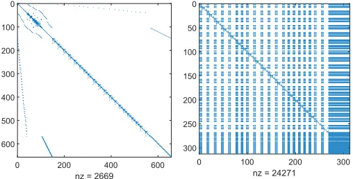
Figure 1. Sparsity ofJ (left) compared toJs(right) in Nordic test system
method) [7]. The shift σ is selected by the user to define the area of the complex plane around which the eigenvalues are sought. In some methods, this shift remains the same throughout the calculations, while in other methods σ is updated to increase accuracy [7].
Computing the state-space matrix Js explicitly requires
eliminating the algebraic states from (4). By doing so, the number of variables is significantly decreased while, at the same time, the sparsity of the system is destroyed. Figure 1 compares the sparsity of J to Js for the Nordic test-system
(Section V-A). It can be seen that while the number of variables is decreased by more than50%, the resulting matrix is almost dense.
While for full space methods the explicit formulation ofJs
is necessary, in iterative methods applying shift-and-inverse, the sparsity of the original matrices can be exploited. It can be shown that [7]:
(Js−σI)y=b⇔(J −σE)
∆V
∆x
=
0
¯
b
(6)
where the elements of b are mapped to ¯b using Γ and the
elements ofyare extracted from∆xin the same manner and correspond to the differential equations of the system. Matrices J andE are defined in Eq. 4.
Using the right hand formulation of (6) allows to exploit the sparsity of matricesJ andE, employ a sparse linear solver, and decrease the computation time of iterative eigenanalysis methods [7].
III. DOMAINDECOMPOSITION-BASEDALGORITHM In this section, a procedure to accelerate the solution of the sparse formulation of (6), using domain decomposition and parallel computing methods, is presented.
A. Power system partitioning
Network M
Injectors Twoport injectors
~ / = / ~
[image:4.612.49.297.51.152.2]M
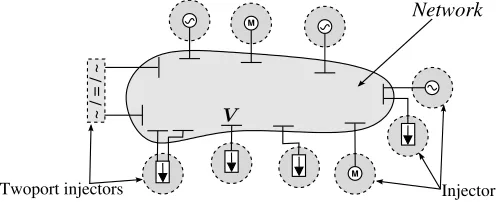
Figure 2. Decomposed power system model
either produce or consume power in normal operating condi-tions and can be attached to a single bus (e.g. synchronous machines, motors, wind-turbines, etc.) or on two buses (e.g. HVDC lines, AC/DC converters, etc.). Hereon, these will be referred to asinjectors.
The proposed decomposition can be visualized in Fig. 2. The scheme chosen reveals a star-shaped, non-overlapping, partition layout. At the center of the star lays the network sub-domain that has interfaces with many smaller sub-sub-domains; the other sub-domains on the other hand only interface with the network sub-domain. This type of partitioning facilitates and simplifies the use of the Schur-complement approach to treat the interface variables [13]. Based on this partitioning, the problem described by Eqs. (1) is decomposed as follows.
The network is described by the algebraic equations:
0=Ψ(x,V) (7)
while the sub-problem of each injector can be described by a DAE problem:
Γix˙i=Φi(xi,V), i= 1, . . . , N. (8)
where xi andΓi are the projections of x andΓ, defined in
(1), on the i-th sub-domain. N is the number of injectors. Due to the star-shaped partition scheme applied, the injectors don’t have dependencies between them but only with the TN through the voltage variablesV.
Thus, the linearized system for the network is formulated:
0=D∆V −
N X
i=1
∆Ii=D∆V − N X
i=1
Ci∆xi (9)
where the interface variables are the rectangular components of the injector currents (∆Ii) andCiis a trivial matrix with zeros
and ones whose purpose is to extract the interface variables from ∆xi. It can be seen thatD=ΨV andCi=Ψxi.
Similarly, the injector linearized systems are formulated:
Γi∆ ˙xi=Ai∆xi+Bi∆V, i= 1, . . . , N. (10)
whereAi=Φixi is the Jacobian of (8) towards its own states
(xi) andBi=ΦiV towards the voltages (V).
B. Decomposed solution
The decomposed linearized systems can be used to perform anequivalent solution of (6). This requires solving together:
D∆V − N X
i=1
Ci∆xi =0 (11a)
(Ai−σΓi)
| {z }
¯
Ai
∆xi+Bi∆V,= ¯bi, i= 1, . . . , N. (11b)
whereb¯i is the projection of¯bon thei-th sub-domain. It can
be seen that the equations are coupled through their interface variables (∆Ii=Ci∆xi and∆V).
For the solution of the decomposed system, Eqs. (11b) are solved for their states (∆xi) and replaced in (11a) formulating
a Schur-complement system:
D−
N X
i=1 CiA¯−
1 i Bi
!
| {z }
¯
D
∆V =− N X
i=1 CiA¯−
1 i b¯i
| {z }
¯
bV
(12)
Then, (12) is solved to get ∆V, which is inserted in (11b), thus decoupling the injectors. The resulting equations can be solved independently for∆xi, and finally the requested vector y can be extracted.
It should be noted, that the Schur-complement matrix D¯ retains the sparsity of D (contrary to Js with J), since the
termsCiA¯− 1
i Biadd only to the already non-zero elements of
the matrix [13]. Thus, a fast sparse linear solver can be used for the solution of (12). In addition, the Schur-complement terms are independent of each other and can be computed in parallel (see Section III-D).
C. Numerical acceleration
Due to the decomposition of the power system model, the solution and update of injectors that do not include any differential equations can be skipped without any effect on the accuracy of the solution. For example, loads are frequently modeled with exponential equations of the type [2]:
P =P0
V V0
α
, Q=Q0
V V0
β
(13)
For these injectors,Γi=0(where 0denotes a matrix with
all zero elements) holds and their state vector xi does not
include any of the solution elements ofy. Thus, if a new shift
σ is given, there is no need to recompute and factorize their matrices. Furthermore, the solution of their states from (11b) can be skipped without sacrificing accuracy.
D. Parallel acceleration
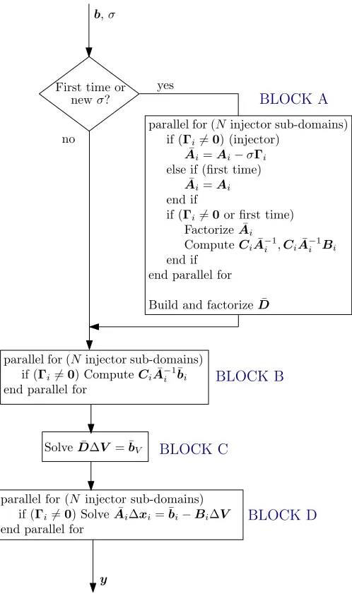
The DPS is sketched in Fig. 3. It receives from the iterative eigenanalysis method vector b and the shift σ, and returns the solution y. This procedure is called several times by the iterative eigenanalysis method.
BLOCK Ais only executed the first time or when the shift
b,σ
First time or newσ?
yes
no
parallel for (Ninjector sub-domains) if (Γi6=0) (injector)
¯
Ai=Ai−σΓi
else if (first time) ¯
Ai=Ai
end if
if (Γi6=0or first time)
Factorize ¯Ai
ComputeCiA¯−
1
i ,CiA¯−
1
i Bi
end if end parallel for
Build and factorize ¯D
parallel for (Ninjector sub-domains) if (Γi6=0) ComputeCiA¯−
1
i ¯bi
end parallel for
Solve ¯D∆V = ¯bV
parallel for (N injector sub-domains) if (Γi6=0) Solve ¯Ai∆xi= ¯bi−Bi∆V
end parallel for
y
BLOCK A
BLOCK B
BLOCK C
[image:5.612.51.300.48.470.2]BLOCK D
Figure 3. Schematic of proposed DPS
with differential equations and the Schur-complement terms are computed. In this block, there are N independent tasks that can be computed in parallel.
The result ofC¯i =CiA¯− 1
i is computed and saved in
mem-ory to be used for the calculation of CiA¯− 1
i ¯bi inBLOCK B.
The Ci of an injector connected to a single bus is a 2×ni
matrix (ni the size ofxi). Thus, the explicit inversion of A¯i
is not necessary and C¯i is calculated by solving the system:
¯
CiT = CiA¯− 1 i
T
= A¯−1
i T
CiT ⇔A¯ T iC¯
T
i =C
T
i (14)
whereT is the conjugate transpose of the complex matrices. In BLOCK B, the contributions to ¯bV of Eq. (12) are
computed in parallel, with N independent tasks. Then, in
BLOCK C, the Schur-complement system is solved for∆V. Finally, in BLOCK D, the linear systems of injectors with differential equations are solved in parallel to obtain∆xi, and
the elements of y are extracted from them.
IV. IMPLEMENTATION SPECIFICS
For the validation of the results obtained using the pro-posed parallel solver on a small test-system, the eigenanalysis method QZ was used through the MATLAB wrappereig.
For the assessment of the proposed parallel solution pro-cedure, theshift-and-invert IRAM was used, provided by the library ARPACK [14] through the MATLAB wrapper eigs. Through the reverse communication interface of ARPACK, the user can provide a subroutine that performs the solution of the sparse system described by (6). Three solvers have been considered: the sparse linear solver SuiteSparse KLU [15], the parallel sparse linear solver PARDISO 5.0.0 [16], and the DPS of Fig. 3. All three solvers are called through MEX interface subroutines.
The parallel solution procedure presented in Section III does not make any assumption on the type of parallel computer. However, for the implementation of the parallel loops in
BLOCKS A,B, andD, the shared-memory parallel computing model has been used to allow the execution on cheap, multi-core, parallel machines (e.g. desktop computers). The OpenMP API was selected as it is supported by most hardware and software vendors and it allows for portable, user-friendly programming [17].
One of the most important tasks is to make sure that parallel threads receive equal amounts of work. Imbalanced load sharing leads to delays, as some threads are still working while others have finished and remain idle. OpenMP includes three predefined mechanisms (namely static, dynamic and
guided) for balancing the work among threads [17].
When the work within each parallel task is the same, the static strategy is preferred. That is, the parallel tasks are assigned to the threads evenly prior to the execution. This strategy has the smallest scheduling overhead cost but can introduce load imbalance if the work inside each task is not equal. When the work within each parallel task is highly imbalanced, the dynamic strategy is preferred. That is, the scheduling is updated during the execution. This strategy has the highest overhead cost for managing the threads but provides the best possible load balancing. Finally, the guided strategy is a compromise between the other two. The schedul-ing in this strategy is dynamic but the number of tasks assigned to each thread is progressively reduced in size [17].
In the proposed solver, there is inherently high imbalance between parallel tasks due to the different sizes of the various injectors. Thus, the dynamic strategy has been chosen for better load balancing. Furthermore, by defining a minimum number of successive tasks to be assigned to each thread (chunks) and positioning the task data consecutively in mem-ory, spatial locality can be exploited. That is, the likelihood of accessing consecutive blocks of memory is increased and the amount of cache misses decreased [17].
g11 g20
g19
g16 g17
g18
g2 g9
g1 g3
g10
g5
g4
g12
g8
g13
g14
g7
g6
g15 4011
4012
1011
1012 1014
1013
1022 1021
2031
cs
4046 4043 4044
4032 4031
4022 4021 4071
4072
4041
1042
1045 1041
4063 4061
1043 1044
4047
4051 4045 4062
TN
DN
NORTH
CENTRAL
EQUIV.
SOUTH
[image:6.612.51.298.48.378.2]4042 2032
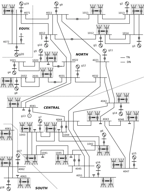
Figure 4. Expanded Nordic model
V. NUMERICALRESULTS
In this section some numerical results are presented. First, the stability and local modes of a Transmission Network (TN) are studied, where the Distribution Networks (DNs) are equivalenced (Section V-A). Then, the same TN is ex-panded with detailed DNs and the effect on its stability and local modes is assessed (Section V-B). The calculations are performed on a 48-core AMD Opteron Interlagos1 desktop computer running Debian Linux 6. The environment variable
OMP_NUM_THREADS is used to vary the number of
com-putational threads. For the IRAM, ten eigenvalues closest to
σ are requested with a toleranceτ = 10−6.
A. Nordic system
This is a variant of the so-called Nordic test system, detailed in [18]. Its one-line diagram is presented in Fig. 4. It is a fictitious system inspired by the Swedish TN in a past configuration. The system model includes a total of 77buses and105branches. Furthermore,20synchronous machines are represented along with generic excitation systems, voltage regulators, power system stabilizers, speed governors, and turbine models. Finally, 23 dynamically modeled loads are included, attached to the distribution buses. The model sums to 1CPU 6238 @ 2.60GHz, 16KB private L1, 2048KB shared per two cores L2 and 6144KB shared per six cores L3 cache, 128GB RAM
Real
-1.5 -1 -0.5 0
Ima
g
in
a
ry
0 2 4 6 8 10
Nordic: QZ method Nordic: IRAM (σ=6.28i)
Expanded Nordic: IRAM (σ=6.28i)
[image:6.612.314.563.49.210.2]ζ=0.05
Figure 5. Eigenanalysis of Nordic and Expanded Nordic systems
-0.5 -0.4 -0.3 -0.2 -0.1 0 0.1 0.2 0.3 0.4 -1
-0.8 -0.6 -0.4 -0.2 0 0.2 0.4
g1 g2g3
g4
g5
g6
g7 g8
g9
g10g11g12g13g14 g15
g16
g17 g18 g19 g20
Figure 6. Nordic: Mode shape of eigenvalue−0.874121 + 5.372230i
656differential-algebraic states, of which312are differential. When decomposing the system, there areN = 43injectors.
Due to the small size of the system, the full spectrum of eigenvalues can be easily computed with the use of QZ method andJs (312×312 matrix). The sparsity of the full (J) and
state-space (Js) Jacobians for this system are shown in Fig. 1.
The eigenvalues of the systems are shown in Fig. 5 with the star markers. The system is small-signal stable, with all eigenvalues in the negative real axis. Moreover, all the local and interarea modes have a dumping ratio2 less than 5%.
Using the IRAM with a shift σ = 0.0, it successfully finds the ten eigenvalues closest to zero. Which include a zero eigenvalue and a cluster of real eigenvalues situated around −0.0155 + 0i. In theory, iterative methods can be used to compute the full eigenvalue spectrum, but the memory and CPU costs would be of the same order as those of the full space methods [19]. Furthermore, several refinement techniques have been proposed to allow the calculation of the rightmost eigenvalues, avoiding stagnation and eigenvalues at infinity. Such techniques have been thoroughly analyzed in other papers, such as [4], [7], and are not considered in this work.
2The dumping ratio of an eigenvalue λ = α + βi is defined as
ζ=−q α
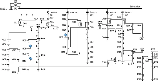
[image:6.612.313.565.243.388.2]TN Bus
Reactor Reactor Reactor Reactor
Substation Tr1
Tr2
Tr3
[image:7.612.50.566.51.313.2]Reactor
Figure 7. Distribution network model used in the expanded Nordic system
Finally, using the IRAM with a shift σ= 6.28i, it is able to find the local modes in the area of0.5−2Hz(shown with square markers in Fig. 5). The right and left eigenvectors of these modes were also computed, to allow for the calculation of the Participation Factors (PFs). The latter are used to deter-mine the degree to which certain states of generators or other devices participate in a selected mode [1]. For this, the IRAM was called twice, using J andJT
respectively. For example, computing the PFs of the local mode−0.874121 + 5.372230i
shows that it is highly influenced by the controls of generator
g6, located in the CENTRAL area. Its corresponding mode shape [1] is shown in Fig. 6.
It should be noted that IRAM with all three solvers finds exactly the same eigenvalues. As mentioned in Section III, the DPS performs an exact solution of system (6), without any approximations.
B. Expanded Nordic system
This section reports on results obtained with a large-scale combined transmission and distribution network model based on the Nordic system presented previously. The TN model is expanded with 146 DNs that replace the aggregated distribu-tion loads (presented in Fig. 4). The model and data of the DNs (sketched in Fig. 7) were taken from [20] and scaled to match the original loads seen by the TN. Multiple DNs were used to match the original loads, taking into account the nominal power of the TN-DN transformers. Each DN includes 100 buses, three PhotoVoltaic (PV) units [21], three type-2 and two type-3 Wind Turbines (WTs) [22], and 133
dynamically modeled loads, namely small induction machines and exponential loads.
In total, the combined transmission and distribution system includes14653 buses,15994 branches,23 large synchronous machines, 438 PVs,730 WTs, and19419 dynamically mod-eled loads. The resulting model has 137186 differential-algebraic states, of which 61298 are differential. When de-composing the system, there are N = 20610 injectors. The penetration of renewable energy sources (here defined as the total active power injected by the PVs and WTs divided by the total load, including the TN loads) reaches 15%.
For this system, the state-space Jacobian matrix Js is
61298 × 61298, which requires inverting a sub-matrix of
75888×75888. MATLAB failed to perform the elimination and supply the matrix to QZ with an error concerning the available memory. Using the IRAM with a shift σ = 0.0, it was able to find ten eigenvalues closest to zero: seven eigenvalues were at 0 + 0i and the remaining at the cluster around −0.0155 + 0i.
Next, with a shift σ = 6.28i, IRAM was able to find the local modes, shown in Fig. 5 with rhombus markers. It can be seen that the local modes are slightly shifted towards more negative real values, but remain close to the ones of the original TN.
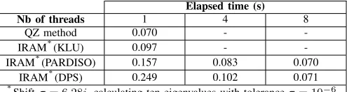
Table I. NORDIC: PERFORMANCE COMPARISON
Elapsed time (s)
Nb of threads 1 4 8
QZ method 0.070 -
-IRAM∗(KLU) 0.097 -
-IRAM∗(PARDISO) 0.157 0.083 0.070
IRAM∗(DPS) 0.249 0.102 0.071
∗
Shiftσ= 6.28i, calculating ten eigenvalues with toleranceτ= 10−6
Table II. EXPANDEDNORDIC: PERFORMANCE COMPARISON
Elapsed time (s)
Nb of threads 1 4 8 16 32 48
QZ method - - -
-IRAM∗(KLU) 41.9 - - - -
-IRAM∗(PARDISO) 50.1 25.7 21.6 19.6 18.6 18.5 IRAM∗(DPS) 98.3 28.3 16.6 10.8 7.7 7.1
∗
Shiftσ= 6.28i, calculating ten eigenvalues with toleranceτ= 10−6
modes by modifying the control parameters of DGs rather than relying on the large generators.
C. Performance comparison
For the smaller Nordic system, the performance of the QZ method and the IRAM with different solvers is shown in Table I. For the QZ method, the time needed for building the state-space Jacobian matrix (Js), calculating the
full-spectrum of eigenvalues and the corresponding left and right eigenvectors, is shown. For the IRAM, the time needed to compute the ten eigenvalues closest to σ = 6.28i and their corresponding left and right eigenvectors is shown. Due to the small size of the system, the QZ method performs really well and the IRAM is not able to compete. Moreover, for these timings, IRAM only calculates ten eigenvalues, while the QZ computes the full spectrum. It is obvious that for such small systems, full space methods are the preferred choice.
Among the IRAM solvers, KLU performs best in sequential mode, while the DPS performs worst. The latter is to be expected, as the DPS has the extra OverHead Cost (OHC) of calculating the Schur-complement terms and bookkeep-ing for the decomposition structure. Some of this OHC is counterbalanced by the numerical acceleration presented in Section III-C. When parallel computing is used, the DPS reaches the performance of PARDISO at 8 threads. Both PARDISO and the DPS do not achieve any better performance, and actually show a slow-down for higher number of threads. This can be explained by the small size of the system which does not offer high parallelization potential compared to the OHC of creating and managing the extra parallel threads.
For the expanded Nordic system, the performance of the IRAM with the different solvers is shown in Table II. Again, in sequential execution the KLU solver is the fastest. The DPS is the slowest due to the extra OHC mentioned above. When more computational threads are used, the DPS becomes faster than PARDISO at 8 threads and at48threads it is2.6 faster; calculating the eigenvalues, left and right eigenvectors in7.1s.
Table III. EXPANDEDNORDIC: DPSPROFILING
% Parallel
Injector shift, factorization, and computation 12.76 YES of Schur-complement terms (BLOCK A)
Addition of Schur-complement terms
2.20 NO
and factorization ofD¯ (BLOCK A)
Computation of¯bV (BLOCK B) 0.95 YES Solution of Schur-complement system 2.15 NO for∆V (BLOCK C)
Solution of injector systems (BLOCK D) 81.95 YES
Total 100.00% 95.66%
In this test case, the DPS is called41times for the computation of the eigenvalues and left eigenvectors and another41times for the right eigenvectors. In total, the Schur-complement terms and the factorization of the injector matrices andD¯ are computed twice, while the solution of the Schur-complement and the injector systems is performed82 times.
The scalability of a single DPS iteration depends on the percentage of work needed for treating the network part (which is in sequential execution) versus the percentage of work for treating the injectors (which is in parallel execution). A profiling of the sequential execution of the solver is shown in Table III. It can be seen that 95.66 % of execution time is spent in the parallel sections of the code. Using Amdahl’s law [23], the DPS can provide a theoretical maximum scalability of
1/(1−0.9566) = 23times, assuming infinite parallel threads and no OHC. Of course, the scalability actually observed is smaller due to the OHC for creating and managing the threads, the limited number of parallel cores, and the extra sequential part in the “non-solver” part of the eigenanalysis method.
Overall, this investigation has shown that for small to medium-scale systems, full-space methods are preferable. While, for large-scale systems on sequential computers, the sparsity of the matrices should be exploited and a fast sparse linear solver (such as KLU) offers significant speedup.
Nevertheless, when parallel computers are available, a higher speedup can be obtained with the use of an “off-the-shelf" parallel solver (such as PARDISO) or a dedicated parallel solver that can extract higher parallelization potential by decomposing the system (such as the proposed DPS). In this work, it was shown that a dedicated decomposed solver can achieve up to 2.6 times higher performance than a state-of-the-art, general, parallel sparse linear solver.
VI. CONCLUSION
Eigenanalysis methods have been used in power systems for stability analysis and the design, tuning, and coordination of controllers. The eigenvalues help to analyze the stability of the system and the existence of oscillatory modes. At the same time, the mode shape and participation factors of these modes can help identify the control parameters that need tuning or coordination [1].
large-scale systems, due to the huge CPU and memory re-quirements. For these systems, iterative methods are frequently used that compute a subset of eigenvalues in a specific area in the complex plane.
In this paper, some methods to accelerate the computation of eigenvalues with iterative methods by exploiting the sparsity of the descriptor systems, have been reviewed. Then, a new parallel solver has been proposed for the solution of sparse lin-ear systems deriving from the computation of eigenvalues. The solver employs domain decomposition and parallel processing techniques to accelerate the solution. It was implemented using the shared-memory parallel model with the use of OpenMP API and tested on a multi-core desktop computer.
The accuracy and performance of the solver was bench-marked against some very fast, sequential and parallel sparse linear solvers, using a small and a large-scale power system models. It was shown that the DPS can achieve high per-formance when employed on multi-core parallel computers, decreasing the eigenanalysis computation time. Such fast com-putations can be useful in external procedures for tuning and coordinating controllers in a closed loop (requiring hundreds of eigenvalue computations).
REFERENCES
[1] M. Gibbard, P. Pourbeik, and D. Vowles,Small-signal stability, control and dynamic performance of power systems. University of Adelaide Press, Adelaide, 2015.
[2] P. Kundur,Power system stability and control. McGraw-hill New York, 1994.
[3] G. H. Golub and C. F. V. Loan,Matrix Computations, 3rd ed. Johns Hopkins University Press, 1996.
[4] J. Rommes, “Arnoldi and Jacobi-Davidson methods for generalized eigenvalue problems Ax = λBxwith singular B,” Mathematics of Computation, vol. 77, no. 262, pp. 995–1016, 2007.
[5] N. Martins, “Efficient Eigenvalue and Frequency Response Methods Applied to Power System Small-Signal Stability Studies,”IEEE Trans-actions on Power Systems, vol. 1, no. 1, pp. 217–224, 1986.
[6] G. Angelidis and A. Semlyen, “Improved methodologies for the calcu-lation of critical eigenvalues in small signal stability analysis,”IEEE Transactions on Power Systems, vol. 11, no. 3, pp. 1209–1217, 1996. [7] J. Rommes and N. Martins, “Exploiting structure in large-scale electrical
circuit and power system problems,”Linear Algebra and its Applica-tions, vol. 431, no. 3-4, pp. 318–333, jul 2009.
[8] M. Bernabeu, M. Taroncher, V. Garcia, and A. Vidal, “Parallel Imple-mentation in PC Clusters of a Lanczos-based Algorithm for an Electro-magnetic Eigenvalue Problem,” in2006 Fifth International Symposium on Parallel and Distributed Computing. IEEE, jul 2006, pp. 296–300. [9] Z. Wu-zhi, S. Xin-li, T. Yong, B. Guang-quan, W. Guo-yang, L. Wei-fang, and L. Tao, “A frequency-domain parallel eigenvalue search algorithm of power systems based on multi-processing,” in2011 IEEE PES Power Systems Conference and Exposition. IEEE, mar 2011. [10] J. Campagnolo, N. Martins, J. Pereira, L. Lima, H. Pinto, and D. Falcao,
“Fast small-signal stability assessment using parallel processing,”IEEE Transactions on Power Systems, vol. 9, no. 2, pp. 949–956, 1994. [11] J. Campagnolo, N. Martins, and D. Falcao, “An efficient and robust
eigenvalue method for small-signal stability assessment in parallel computers,” IEEE Transactions on Power Systems, vol. 10, no. 1, pp. 506–511, 1995.
[12] X. Zhang and C. Shen, “A Distributed-computing-based Eigenvalue Algorithm for Stability Analysis of Large-scale Power Systems,” in2006 International Conference on Power System Technology, oct 2006. [13] P. Aristidou, D. Fabozzi, and T. Van Cutsem, “Dynamic Simulation of
Large-Scale Power Systems Using a Parallel Schur-Complement-Based Decomposition Method,”IEEE Transactions on Parallel and Distributed Systems, vol. 25, no. 10, pp. 2561–2570, oct 2013.
[14] R. Lehoucq, D. Sorensen, and C. Yang, “ARPACK SOFTWARE.” [Online]. Available: http://www.caam.rice.edu/software/ARPACK/ [15] T. A. Davis and E. P. Natarajan, “Algorithm 907: KLU, A Direct
Sparse Solver for Circuit Simulation Problems,”ACM Transactions on Mathematical Software, vol. 37, no. 3, pp. 1–17, sep 2010.
[16] A. Kuzmin, M. Luisier, and O. Schenk, “Fast Methods for Computing Selected Elements of the Green’s Function in Massively Parallel Nano-electronic Device Simulations,” in2013 Euro-Par Parallel Processing. Springer Berlin Heidelberg, 2013, pp. 533–544.
[17] B. Chapman, G. Jost, and R. Van Der Pas,Using OpenMP: Portable Shared Memory Parallel Programming. MIT Press, 2007.
[18] T. Van Cutsem and L. Papangelis, “Description, Modeling and Simulation Results of a Test System for Voltage Stability Analysis,” University of Liege, Tech. Rep., 2013. [Online]. Available: http://hdl.handle.net/2268/141234
[19] J. Rommes, N. Martins, and F. Freitas, “Computing rightmost eigenval-ues for small-signal stability assessment of large-scale power systems,”
IEEE Transactions on Power Systems, vol. 25, no. 2, pp. 929–938, 2010. [20] A. Ishchenko, “Dynamics and stability of distribution networks with dispersed generation,” Ph.D. dissertation, Eindhoven University of Tech-nology, 2008.
[21] A. Ellis, M. Behnke, and C. Barker, “PV system modeling for grid plan-ning studies,” in2011 37th IEEE Photovoltaic Specialists Conference. IEEE, jun 2011, pp. 2589–2593.
[22] WECC, “Wind Power Plant Dynamic Modeling Guide,” Western Elec-tricity Coordinating Council (WECC), Tech. Rep., 2014.