Simulation of supercritical Diesel jets using the PC-SAFT EoS

City, University of London Institutional Repository

Citation

: Rodriguez, C., Koukouvinis, F. ORCID: 0000-0002-3945-3707 and Gavaises, M.

ORCID: 0000-0003-0874-8534 (2018). Simulation of supercritical Diesel jets using the

PC-SAFT EoS. The Journal of Supercritical Fluids, doi: 10.1016/j.supflu.2018.11.003

This is the published version of the paper.

This version of the publication may differ from the final published

version.

Permanent repository link:

http://openaccess.city.ac.uk/id/eprint/21043/

Link to published version

: http://dx.doi.org/10.1016/j.supflu.2018.11.003

Copyright and reuse:

City Research Online aims to make research

outputs of City, University of London available to a wider audience.

Copyright and Moral Rights remain with the author(s) and/or copyright

holders. URLs from City Research Online may be freely distributed and

linked to.

City Research Online:

http://openaccess.city.ac.uk/

[email protected]

Contents lists available atScienceDirect

The Journal of Supercritical Fluids

journal homepage:www.elsevier.com/locate/supflu

Simulation of supercritical diesel jets using the PC-SAFT EoS

C. Rodriguez

_{, P. Koukouvinis, M. Gavaises}

School of Mathematics, Computer Science & Engineering, Department of Mechanical Engineering & Aeronautics, City University London, Northampton Square EC1V 0HB, United Kingdom

G R A P H I C A L A B S T R A C T

A R T I C L E I N F O

Keywords:

Supercritical PC-SAFT EoS Diesel fuel injection

A B S T R A C T

A numerical framework has been developed to simulate supercritical Diesel injection using a compressible density-based solver of the Navier-Stokes equations along with the conservative formulation of the energy equation. Multi-component fuel-air mixing is simulated by considering a diffused interface approximation. The thermodynamic properties are predicted using the Perturbed Chain Statistical Associating Fluid Theory (PC-SAFT) real-fluid equation of state (EoS). This molecular-based EoS requires three empirically determined but well-known parameters to model the properties of a specific component, and thus, there is no need for extensive model calibration, as is typically the case when the NIST library is utilised. Moreover, PC-SAFT can handle flexibly the thermodynamic properties of multi-component mixtures, which is an advantage compared to the NIST library, where only limited component combinations are supported. This has allowed for the properties of Diesel fuel to be modelled as surrogates comprising four, five, eight and nine components. The proposed nu-merical approach improves the overall computational time and overcomes the previously observed spurious pressure oscillations associated with the utilization of conservative schemes. In the absence of experimental data, advection test cases and shock tube problems are included to validate the developed framework. Finally, two-dimensional simulations of planar jets of n-dodecane and a four component Diesel surrogate are included to demonstrate the capability of the developed methodology to predict supercritical Diesel fuel mixing into air.

1. Introduction

Diesel fuel injection at supercritical state in the combustion

chamber is known to improve fuel-air mixing as the fluid diffusivity is much higher than that of molecules in liquid phase [1]. Moreover, the studies of [1–4] have shown how injection at these conditions can

https://doi.org/10.1016/j.supflu.2018.11.003

Received 6 July 2018; Received in revised form 2 November 2018; Accepted 3 November 2018 ⁎_{Corresponding author.}

E-mail address:[email protected](C. Rodriguez).

Available online 13 November 2018

0896-8446/ © 2019 The Authors. Published by Elsevier B.V. This is an open access article under the CC BY-NC-ND license (http://creativecommons.org/licenses/BY-NC-ND/4.0/).

reduce the emissions of particulate matter and nitrogen oxides. Building upon these findings, the aim of the present research is to develop a numerical framework to simulate supercritical Diesel-air mixing pro-cesses where the liquid evaporation step is circumvented. A mixture or a single-component reaches a supercritical state when both pressure and temperature surpass its critical properties. In the critical region, repulsive interactions overcome the surface tension resulting in the existence of a single-phase that exhibits properties of both gases and liquids. To simulate such cases of supercritical and transcritical jets, commonly diffuse interface methods are employed [5–7]. Three main difficulties are associated with the numerical simulation of such cases: (i) the treatment of large density gradients, (ii) the need of using a real-fluid EoS and (iii) the elimination of spurious pressure oscillations, typically occurring in simulations when fully conservative (FC) schemes are employed along with real-fluid EoS [8].

With regards to large density gradients, high order reconstruction methods can be used to describe sharp changes. In [9] the authors performed a two-dimensional large-eddy simulation (LES) of super-critical mixing and combustion employing a fourth-order flux-differ-encing scheme and a total-variation-diminishing (TVD) scheme in the spatial discretization. Similarly, in [10] a fourth-order central differ-encing scheme was applied together with a fourth-order scalar dis-sipation; this was found to stabilize the simulation of a cryogenic fluid injection and mixing under supercritical conditions. Moreover, in the work of [11] an eighth-order finite differencing scheme was employed in order to simulate homogeneous isotropic turbulence under super-critical pressure conditions. Furthermore, in [12] a density-based sensor was employed, which switches between a second-order ENO (Essentially non- oscillatory) and first-order scheme to suppress the oscillations. In the present study a fifth-order WENO (Weighted Es-sentially Non-Oscillatory) scheme is applied in the 2D (two-dimen-sional) simulations due to its high order accuracy and non-oscillatory behaviour.

Moving to the second issue, typically cubic EoS models like the Peng-Robinson (PR) [13] and Soave-Redlich-Kwong (SRK) [14] are used in supercritical and transcritical simulations. For example, in [7,15–17], the SRK EoS was employed to close the N–S equations and compute the fluid properties under supercritical and transcritical con-ditions. Similarly, in [6,8,12,18] the non-ideal fluid behavior was modelled by applying the PR EoS. Nevertheless, cubic models com-monly present low accuracy for computing the thermodynamic prop-erties of hydrocarbons at high density ranges and temperatures that are

typical for today’s high pressure fuel injection systems [5]. To overcome these difficulties, the Statistical Association Fluid Theory Equation of State (SAFT EoS) can be employed. Several papers have been published pointing out the advantages of the SAFT models with respect to cubic EoS. For example [19], describes how the PC-SAFT model is better than cubic EoS for predicting gas phase compressibility factors and oil phase compressibilities. In [20] the superiority of the PC-SAFT performance is demonstrated relative to the Cubic Plus Association (CPA) EoS in cor-relating second order derivative properties, like speed of sound, dP/dV and dP/dT derivatives, heat capacities and the Joule–Thomson coeffi-cient in the alkanes investigated. Similarly [21], points out the super-iority of the SAFT-BACK EoS over the PR EoS, particularly at high-density conditions, for computing second order derivative properties such as sound velocity and isobaric and isochoric properties. The study of [22] states that cubic EoS predict a linear increase of the Z factor (compressibility factor) with pressure, while the PC-SAFT EoS shows a better pressure dependence. Finally [23], shows how the sPC-SAFT (simplified PC-SAFT) is more precise than SRK and CPA to compute the speed of sound of normal alkanes and methanol. The SAFT EoS is based on the perturbation theory, as extensively studied in [24–27] by Wer-theim. The authors of [28,29], developed this EoS by applying Wer-theim’s theory and extending it to mixtures. In this method, each mo-lecule is decomposed into spherical segments of equal size to form a repulsive, hard sphere reference fluid. Next, the attractive interactions between segments are added to the model. Finally, the segment-seg-ment energy needed to form a chain between the hard-sphere fluid segments is added to the model; if the segments exhibit associative interactions such as hydrogen bonding, a term for this interaction is also included. Among the different variants of the SAFT model, the PC-SAFT is the one implemented here. In this model, hard chains are used as the reference fluid instead of hard spheres. While the SAFT EoS computes segment-segment attractive interactions, the PC-SAFT EoS computes chain-chain interactions, which improves the thermodynamic description of chain-like, fluid mixtures [30]. The main issues of using a complex EoS are the difficult implementation and the high computa-tional cost [6]. Some tabulation methods have been developed for single-species cases [31] but these approaches cannot be utilised with mixtures of more than two components. In this research, the Diesel properties are modelled using surrogates of four, five, eight and nine components so employing tables is not an option. The use of the double-flux model of [6,8,32] can significantly reduce the required computa-tional time as the complex EoS is employed only once in the hyperbolic

Nomenclature

List of abbreviations

CFD Computational Fluid Dynamics CFL Courant–Friedrichs–Lewy ENO Essentially Non-Oscillatory EoS Equation of State

FC Fully Conservative

HLLC Harten-Lax-van Leer-Contact LES Large Eddy Simulation N–S Navier-Stokes PR Peng-Robinson

PC-SAFT Perturbed Chain Statistical Associating Fluid Theory QC Quasi-Conservative

RK2 Second-order Runge–Kutta SRK Soave-Redlich-Kwong

SSP-RK3 Third-order strong-stability-preserving Runge–Kutta TVD Total Variation Diminishing

VLE Vapor-Liquid Equilibrium

WENO Weighted Essentially Non-Oscillatory

List of Symbols

a˜res _{Reduced Helmholtz free energy [-]}

a _{Speed of sound [m s-1]}

d Temperature-dependent segment diameter [Å]

g Radial distribution function [-] I Integrals of the perturbation theory [-]

k Boltzmann constant [J/K] m Number of segments per chain [-]

m¯ Mean segment number in the system [-]

p Pressure [Pa]

R Gas constant [J mol-1 K-1]

T Temperature [K]

xi Mole fraction of component i [-] Z Compressibility factor [-]

U Conservative variable vector F x-convective flux vector

G y-convective flux vector FV x-diffusive flux vector

operator of the numerical model per time step [33]. However, recently it has been reported that the large energy conservation error in quasi-conservative (QC) schemes produces an unphysical quick heat-up of the jet [5] and thus, making these schemes inadequate for Diesel injection simulations where the temperature plays a significant role on de-termining the ignition time. The FC formulation proposed in this paper reduces the number of times the EoS is employed, making it possible to use complex EoS in affordable CPU time.

Finally, referring to the third issue of the spurious pressure oscil-lations, several papers have tried to address this problem. The work of [7] utilised a QC formulation, which solves a pressure evolution equation instead of the energy conservation equation. In [34] the au-thors applied a QC framework where the artificial dissipation terms in the mass, momentum and energy equations are related and the pressure differential is zero. The authors of [35] developed the double flux model to avoid spurious pressure oscillations in compressible multi-component simulations where the perfect gas EoS is applied. In [36] they extended it to reactive flows while in [6,8,32] it was extended to real fluids and transcritical conditions. The current paper proposes a modification to the calculation of the pressure and sonic fluid velocity at the cell faces in FC formulations; this is found to smooth-out the spurious pressure oscillations observed with previous methods. Ad-ditionally, it reduces the overall computational time allowing simula-tions of multicomponent Diesel surrogate fuels to be performed. The composition of the Diesel surrogates employed here has been proposed by [37]; they are divided into two types, depending on how closely the surrogates match the composition of real Diesel.

To the best of the author’s knowledge, this is the first time that the PC-SAFT EoS is used to simulate supercritical injections of Diesel modeled as a multi-component surrogate. The structure of the paper is as follows. Initially, the numerical method is presented, followed by 1D (one-dimensional) verification test cases. Advection test cases and shock tube problems are included to show the overall performance of the developed framework and evaluate how the number of compounds of the Diesel surrogate employed affects the accuracy of the results. Then, two-dimensional simulations of planar jets of n-dodecane and a four component Diesel surrogate are included to demonstrate the cap-ability of the scheme to predict supercritical Diesel fuel mixing into air.

2. Numerical method

The Navier-Stokes equations for a non-reacting multi-component mixture containing N species in a x–y 2D Cartesian system are given by:

+ + = +

t x y x y

U F G Fv Gv

(1) The vectors of Eq.1are:

= = + + = + + = + Y Y u E uY uY u p u

E p u

Y Y u p E p J J u q

U , F G F

( )

,

( )

, ,

N N N

x

x N xx xy xx xy x v 1 1 2 1 2 ,1 , (2) = + J J

u v q

G

y

y N yx yy yx yy y

v

,1

,

whereρis the fluid density,uandvare the velocity components, p is the pressure,Eis the total energy,Jiis the mass diffusion flux of species i, σ is the deviatoric stress tensor andqis the diffusion heat flux vector. The finite volume method has been utilised for solving the above

equations on a Cartesian numerical grid. As mentioned, the PC-SAFT EoS is utilised to approximate thermo-physical properties. Moreover, operator splitting as described in [38] is employed to separate the hy-perbolic and parabolic operators. The global time step is computed using the CFL (Courant-Friedrichs-Lewy) criterion of the hyperbolic part. The developed numerical framework considers a condition of thermodynamic equilibrium in each cell. The way the PC-SAFT EoS has been coupled with the Navier-Stokes equations is described in [33]. Phase separations or metastable thermodynamic states are beyond the scope of this research and are not considered.

2.1. CFD code

2.1.1. Hyperbolic sub-step

The HLLC (Harten-Lax-van Leer-Contact) solver is applied to solve the Riemann problem. In density based codes, once the spatial re-construction scheme has been used to compute the left and right states of the Riemann problem, the EoS is applied to compute the pressure and sonic fluid velocity at both sides (considering that the conservative variables have been reconstructed). Eq.3shows the pressure expressed in a form equivalent to a general EoS [7]:

= +

p( , , )e Yi F( , )Y ei G( , )Yi (3)

However, the computed pressure may present a large error if the functions F or G depend on the interpolated conservative variables. Even in single-species cases, if these functions are density-dependent and consist of high-order density terms, a small change in the inter-polated density can produce large variations in the calculated pressure. The incorrect pressure introduces an error in the computation of the fluxes, which finally generate spurious oscillations during the numer-ical solution. In the present study, this is avoided by reconstructing the primitive variables (or only the pressure) and the conservative variables at the cell faces at the same time. This simple modification has been found to smooth-out the spurious pressure oscillations generated by the high-nonlinearity of the EoS.

By reconstructing the pressure, the only variable left to compute the fluxes at the cell faces is the speed of sound. Instead of using the EoS to calculate this variable, the sonic fluid velocity is interpolated using cell centre values as well. Therefore, the PC-SAFT EoS is used only once per cell in each RK sub-time step, thus reducing significantly the compu-tational time. A detailed description of the spatial reconstruction methods and temporal integration employed can be found in the Appendix.

2.1.2. Parabolic sub-step

The method of [39] is used to calculate the dynamic viscosity and the thermal conductivity. The diffusion coefficient is calculated em-ploying the model developed by [40]. Linear interpolation is performed for computing the conservative variables, temperature and enthalpy on faces from cell centres. The viscous stress tensor is calculated as:

= + = + = = +

(

)

(

)

(

)

xx u_x u_x v_y

yy v_y u_x v_y

xy yx u_y v_x

2 3 2 3

(4) whereµ is the shear viscosity. Effects of bulk viscosity are not con-sidered as, to the best of the author’s knowledge, accurate models are not available.

The species mass diffusion flux of species i is calculated as: = D Y

Ji i i (5)

whereDis the diffusion coefficient. The heat flux vector is calculated as:

= T h D Y q

i N

i i i

(6) where is the thermal conductivity andhis the enthalpy.

2.2. Diesel surrogates

Table 1shows a comparison between the experimentally measured surrogate densities computed at 293.15 K and 0.1 MPa with the den-sities calculated employing the EoS-based method developed at NIST [41] and the PC-SAFT EoS. The composition of the Diesel surrogates was proposed by [37]. They are divided into two accuracy types de-pending on how close their composition is to real Diesel. More speci-fically, V0a and V0b are two low-accuracy surrogates and V1 and V2 are the two high-accuracy surrogates. Their molar composition is summarized inTable 6. The results obtained by the PC-SAFT EoS shows the highest degree of agreement with the experimental values [42] in comparison with the results obtained by [37] applying the method developed at NIST.

2.3. Phase diagrams

The number of phases is solved by an isothermal flash calculation after a stability analysis using the Tangent Plane Criterion Method proposed by [43] and applied to the PC-SAFT EoS by [44] using the code developed by [42]. This methodology has not been implemented in the CFD code. It is used to obtain the phase diagrams employed to check that the vapor-liquid equilibrium (VLE) state is not present in the solution of the performed simulations (Fig. 1).

3. Results

Firstly, a comparison of the temperature, sonic fluid velocity and internal energy of n-dodecane, V0a, V0B, V1 and V2 Diesel surrogates is presented to point out the importance of an accurate fuel properties modelling. Then, several advection test cases and shock tube problems are solved to validate the hyperbolic part of the numerical framework and show how the reconstruction technique explained in Section2.1

smooths-out the spurious pressure oscillations. Finally, two-dimen-sional simulations at high-load Diesel operation conditions of super-critical n-dodecane and Diesel surrogate V0A are presented to demon-strate the multicomponent and multidimensional capability of the developed numerical solver.

3.1. Dodecane and diesel comparison

Fig. 2shows a comparison of the thermodynamic properties of n-dodecane and the Diesel surrogates V0A, V0B, V1 and V2 at 6 MPa, as calculated using the PC-SAFT EoS. The main differences between do-decane and the Diesels can be found in the temperature and sonic fluid velocity at high densities. The temperature is an important thermo-dynamic property in transcritical simulations because it determines the transition to a supercritical state. The sonic fluid velocity plays a key role in the computation of the hyperbolic fluxes and in the time step calculation. The effects that these variables have on the CFD results can be seen later in the paper, inFig. 12.

3.2. Advection test cases

3.2.1. Single-species advection test case

Table 2summarises the advection test cases simulated.Fig. 3shows the results of the Advection Test Case 1, where Nitrogen is used. The initial conditions are the same as the ones used by [15] in the interface advection problem. The computational domain is x ε [0,1] m. In 0.0 < x < 0.3 m, the initial conditions are ρ = 450 kg/m3_{, p = 4 MPa,}

and u = 10.0 m/s; in the rest of the domain they are ρ = 45.0 kg/m3_,

p = 4 MPa, and u = 10.0 m/s. A uniform grid spacing of 0.01 m is employed; the simulated time is t = 0.04 s; the CFL is set to be 0.5. Wave transmissive boundary conditions are implemented in the left and right sides of the computational domain. The spatial reconstruction has been performed in two different ways. In the first one, the PC-SAFT EoS is used to compute the sonic fluid velocity and the pressure using the reconstructed conservative variables. In the second one, the pressure and sonic fluid velocity are interpolated onto the cell faces, as described in Section2.1.

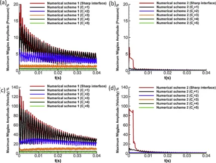
Large wiggles appear in the velocity and pressure fields at 0.04 s using the classic spatial reconstruction method, as can be seen inFig. 3. The start-up error is present for a long period of time in the simulation and contaminate the solution. This can be observed in theFigs. 4 and 5, which both reveal the maximum wiggles amplitude (calculated as the maximum difference between the analytical solution and the computed profile [15]) along time in the pressure and velocity fields. More spe-cifically, Fig. 4presents the results obtained using the second-order MUSCL-Hancock scheme while inFig. 5the fifth-order WENO scheme has been utilised. By applying the schemes proposed in Section2.1. and explained in the Appendix, once the oscillations generated by the start-up error have travelled start-upstream and downstream with their char-acteristic speeds and reach the boundaries of the computational do-main, the solution shows no wiggles. A smooth initial interface can be used for avoiding the initial start-up error [46]. When employing a diffuse interface method, the interfaces are not sharp one-point jumps but smooth as they are resolved. Then, a smooth initial profile is a realistic initial condition. To initialize the simulation using a smooth interface the primitive variables are calculated employing the following formula [46]:

= +

q qL(1 fsm) q fR sm (7)

= +

f (1 erf[ R/ ])

2

sm ₍₈₎

where L and R refers to the left and right interface conditions and Ris the distance from the initial interface. =C x, where x is the grid spacing andC is a free parameter to determine the interface smooth-ness. Employing this formula, the number of grid points used in the initial interface does not depend on the grid resolution. The interface will be sharpened in space if the number of cells utilised is increased but the number of points across the interface does not change.Fig. 4 and 5

show that for the spatial reconstruction methods proposed the start-up error is not present in the obtained solution for values ofC bigger than 2.

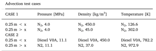
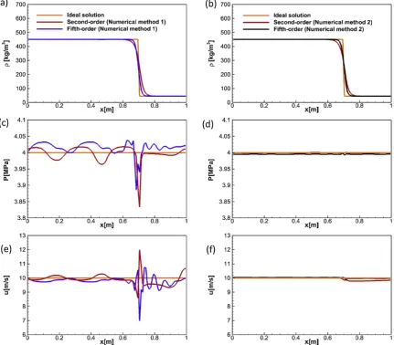
3.2.2. Multi-component advection test case

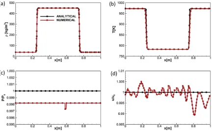
Fig. 7shows the results of the advection of the Diesel surrogate V0A in nitrogen (Table 2). The computational domain is xε [0,1]m; the initial conditions in 0.25 m < x < 0.75 m are ρV0A= 450.0 kg/m3,

pV0A= 11.1 MPa, and TV0A= 782.2 K; in the rest of the domain

ρN2= 37.0 kg/m3, pN2= 11.1 MPa, and TN2= 972.9 K. The advection

velocity utilised is 10 m/s; periodic boundary conditions are used; 500 cells are employed; the simulated time is t = 0.1 s; the fifth-order WENO discretization scheme presented is used; and the CFL is set to be 0.5. A smooth interface is applied(C =2).The oscillations in the ve-locity and pressure field are lower than 1.0% and 0.3% respectively of

Table 1

Comparison between experimentally measured surrogate densities (kg/m3) at 293.15 K and 0.1 MPa with the NIST and PC-SAFT predictions [42].

Surrogate Experiment NIST PC-SAFT

V0a 818 809.1 814.9

V0b 837.5 821.6 833.2

V1 828.4 814.1 825.2

the initial values. The vapor-liquid equilibrium (VLE) state is not pre-sent in the solution, as can be seen in Fig. 6 where the maximum temperature encountered by the Diesel surrogate V0A - nitrogen phase boundary at 7 MPa is 705 K (this value is lower at higher pressures). The minimum temperature reached in the simulation is 782k.

3.3. Shock tube problems

The Euler equations are solved in this exercise, so direct comparison with the exact solver can be performed in order to validate the hy-perbolic part of the developed numerical framework. The exact solution has been computed using the methodology described in [47]. 3.3.1. Shock tube problem 1, 2, 3

Fig. 8–11displays the results of three shock tube problems which

employs dodecane as working fluid. The domain is xε[-0.5, 0.5] m; 1000 equally spaced cells were used. Wave transmissive boundary conditions are implemented in the left and right sides. The initial Fig. 1.Experimental [45] and calculated pressure-composition phase diagram for the N2(1) + C12H26(2) system. Solid lines: PC-SAFT EoS with kij= 0.1446 [33].

Fig. 2.Comparison of thermodynamic properties of n-dodecane and Diesel surrogates at 6 MPa: (a) density, (b) sonic fluid velocity, (c) internal energy. Table 2

Advection test cases.

Advection test cases

CASE 1 Pressure [MPa] Density [kg/m3_{] Temperature [K]}

0.25 m < x N2, 4.0 N2, 450.0 N2, 126.6

0.25 m > x N2, 4.0 N2, 45.0 N2, 302.0

CASE 2

0.25 m < x Diesel V0A, 11.1 Diesel V0A, 450.0 Diesel V0A, 782.2 0.25 m > x N2, 11.1 N2, 37.0 N2, 972.9

conditions are summarized inTable 3. The simulated time is 5 10−4_{s in}

the Shock Tube Problem 1 and 2, and 2.5 10−4_{s in the Shock Tube}

Problem 3. The CFL is set to 0.3 to stabilize the cases with large spur-ious pressure oscillations. The reconstruction step has been performed in two different ways. In the first one, the PC-SAFT EoS is used to compute the sonic fluid velocity and the pressure using the re-constructed conservative variables. In the second one, the pressure and sonic fluid velocity are interpolated onto the cell faces, as described in Section2.1.

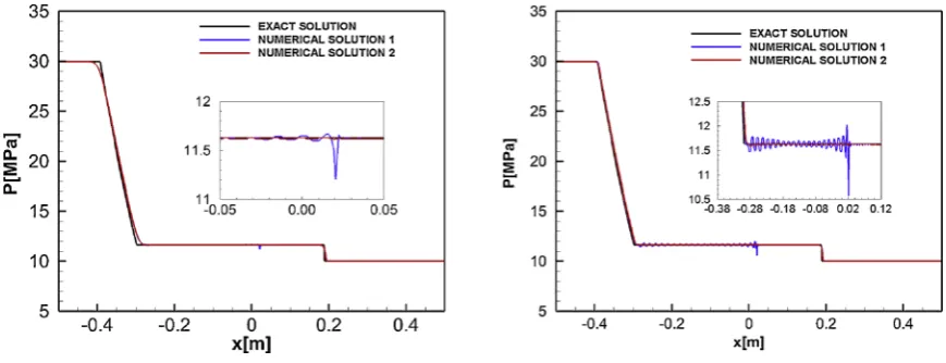
In the Shock Tube Problem 1 (Figs. 8 and 9), the variation of the thermodynamic properties between the right and left states is not large enough to generate spurious pressure oscillations. However, spurious pressure oscillations appear in the Shock Tube Problem 2 (Fig. 10) because of the sharper jump in the thermodynamic conditions. When employing the modified reconstruction, the spurious oscillations are significantly reduced. In the Shock Tube Problem 3 the larger variation in the thermodynamic properties between the left and right states provoke the formation of large spurious pressure oscillations. Using the modified reconstruction, the oscillations can be significantly reduced (especially when the MUSCL- Hancock scheme is employed) like in the Shock Tube Problem 2.

3.3.2. Shock tube problem 4

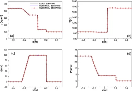
Fig. 12displays the density, temperature, pressure, velocity, sonic fluid velocity and internal energy results of a transcritical shock tube

problem, which employs dodecane and the V0A, V0B, V1 and V2 Diesel surrogates as working fluids. The composition of the Diesel surrogates is summarized inTable 6. The domain is xε[0,1]m.800equally spaced cells were used. Wave transmissive boundary conditions are im-plemented in the left and right sides. The initial conditions in the left state are ρL= 620 kg/m3, pL= 30 MPa, uL= 0 m/s; and in the right state are ρR= 100 kg/m3_{, pR= 10MPa, uR= 0 m/s. The fifth-order} WENO discretization scheme presented in Section2.1. is used. The CFL is set to 0.8. The simulated time is 5 10−4_s.

The obtained results suggest that there is a significant difference between dodecane and the Diesel surrogates. The temperatures com-puted using Diesel surrogates are higher than those obtained for do-decane throughout the whole computational domain. The different sonic fluid velocities in the high-density region forces the expansion wave to move with different velocities. The larger variations in the Diesel internal energy may be related to the different velocity profiles computed. There is not a significant difference in the results obtained using the different Diesels.

The PC-SAFT EoS is implemented using loops that depend on the number of components solved, which means that it takes more time to compute the properties of mixtures. This is the reason why the Diesel surrogate V0A will be used in the 2D simulation, as the results obtained using the two low accuracy surrogates (V0a and V0b) and the two high-accuracy surrogates (V1 and V2) are practically the same. The Diesel surrogate V0A is the one with less compounds.

Fig. 3.Advection Test Case 1 (N2), CFL = 0.5, u = 10 m/s, 100 cells, t = 0.04 s. Comparison of the (a–b) density, (c–d) pressure and (e–f) x-velocity between the

Fig. 4.Advection Test Case 1 (N2), CFL = 0.5, u = 10 m/s, 100 cells. Maximum wiggles amplitude in the velocity (c-d) and pressure (a-b) fields. Analysis of smooth

and sharp initial interfaces using the second-order MUSCL-Hancock scheme.

Fig. 5.Advection Test Case 1 (N2), CFL = 0.5, u = 10 m/s, 100 cells. Maximum wiggles amplitude in the velocity (c-d) and pressure (a-b) fields. Analysis of smooth

and sharp initial interfaces using the fifth-order WENO scheme.

3.4. Two-dimensional cases

The results of planar two-dimensional injections are presented in this section. As mentioned earlier, the fuels employed are n-dodecane and the Diesel surrogate V0A. A structured mesh is applied with a uniform cell distribution. The cell size is 5.5 μm × 5.5 μm. The domain used is 5 mm × 2.5 mm. The parabolic sub-step is included into these simulations, without sub-grid scale modelling for turbulence or heat/ species diffusion. The CFL number is set at 0.5. The fifth-order WENO discretization scheme presented in Section 2.1. is used. Transmissive boundary conditions are applied at the top, bottom and right bound-aries while a wall condition is employed at the left boundary. A flat velocity profile is imposed at the inlet. The velocity of the jet is 200 m/s and the diameter of the exit nozzle is 0.1 mm. 405,000 cells are em-ployed.

3.4.1. Dodecane jet

A multicomponent simulation has been included to prove the

multi-species capability of the developed framework. According to the clas-sification of [49], all binary N2+ hydrocarbon fluid mixtures are Type III except for methane. Starting at the critical point of n-dodecane, the critical pressure of a N2+ n-dodecane mixture grows by increasing the

nitrogen concentration [50]. It reaches higher pressures than the ones observed in Diesel engine combustion chambers (Fig. 1). Thus, to avoid the VLE state the dodecane is injected at a temperature higher than its critical value in the performed simulation.

The case is initialized using a pressure in the chamber of 11.1 MPa; the density and the temperature of the nitrogen in the chamber are 37.0 kg/m3 _{and 973 K (high-load Diesel operation conditions [51]),}

respectively. The density and temperature of the jet are 400.0 kg/m3

and 736.8 K, seeTable 4.

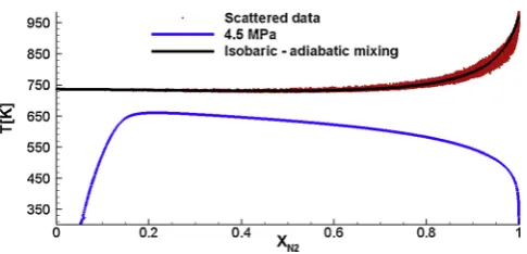
The Kelvin Helmholtz instability is developing in the shear layer, as it can be seen inFig. 13. No pressure oscillations appear in the results. The jet is quickly heated-up from a liquid-like supercritical state to a gas-like supercritical state. A comparison of averaged scattered data of composition and temperature and an isobaric-adiabatic mixing process can be seen in Figs. 14 and 15. As [52] stated, fully conservative schemes describe an adiabatic mixing process. The isobaric-adiabatic line was computed using Eqs.9–10and the initial conditions of this case:

= +

=

m m m

m mass flow rate

3 1 2

(9)

= +

=

m h m h m h

h specific enthalpy

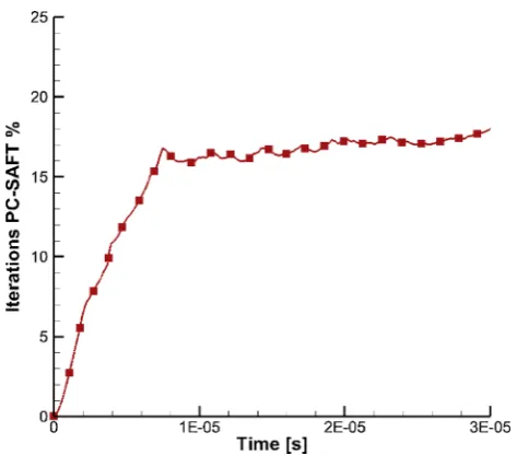
3 3 1 1 2 2

(10) The number of times the PC-SAFT model is solved in the hyperbolic operator per time step is lower than 20% the times it is employed using a classic FC implementation. As already mentioned, by interpolating the pressure and sonic fluid velocity at the cell faces, the EoS has to be solved once per cell in each RK sub-time step instead of once per cell face in the hyperbolic operator. Additionally, in many cells the EoS is Fig. 6.Diesel surrogate V0A - nitrogen phase boundary from VLE at different

pressures.

Fig. 7.Advection Test Case 2 (Diesel surrogate V0A – N2), CFL = 0.5 u = 10 m/s, 500 cells, t = 0.1 s. Comparison of the (a) density, (b) temperature, (c) pressure and

Fig. 8.Shock Tube Problem 1 (MUSCL-Hancock scheme, Dodecane). CFL = 0.5, u = 10 m/s, 1000 cells, t = 5 10−4_{s. Comparisons of (a) density, (b) temperature,}

(c) velocity and (d) pressure profiles: exact solution and numerical solutions. Numerical solution 1: Pressure and sonic fluid velocity computed at the faces using the EoS. Numerical solution 2: Pressure and sonic fluid velocity interpolated at the faces.

Fig. 9.Shock Tube Problem 1 (Fifth-order WENO, Dodecane). CFL = 0.3, 1000 cells, t = 5 10−4_{s. Comparisons of (a) density, (b) temperature, (c) velocity and (d)}

pressure profiles: exact solution and numerical solutions. Numerical solution 1: Pressure and sonic fluid velocity computed at the faces using the EoS. Numerical solution 2: Pressure and sonic fluid velocity interpolated at the faces.

not used to update the temperature, pressure, sonic fluid velocity and enthalpy values as the sum of the fluxes is approximately 0 (Appendix). This can be clearly observed inFig. 16. The significant reduction on the number of times the PC-SAFT model has to be solved allows to carry out simulations at affordable CPU times using a FC formulation. In the cases presented here, the time taken to solve 3.5 × 10−5_{s were 93.8 hours on}

a single CPU.

3.4.2. Diesel surrogate V0A jet

This case is initialized using a pressure in the chamber of 11.1 MPa; the density and the temperature of the nitrogen in the chamber are 37.0 kg/m3 _{and 973 K (high-load Diesel operation conditions [51]),}

respectively. The density and temperature of the jet are 490.0 kg/m3

and 742 K (Table 4). The temperatures encountered along the simula-tion are higher than the temperatures at which VLE exists, as can be seen in the previousFig. 6. The binary interaction parameter used be-tween the nitrogen and the Diesel compounds is the same one used in the nitrogen-dodecane mixture (kij = 0.1446).

Fig. 17shows the density, temperature and pressure at 3.4 × 10−5

s. For this multi-component fuel simulations, the time taken to solve 3.5 × 10−5_{s were 165 h on the same CPU utilised for the dodecane}

simulation (∼75% longer). By knowing the mass fractions in each cell, it is possible to determine how many components are present in a cell a priori. The PC-SAFT is then only solved for that specific number of components. Most cells along the simulation in the combustion chamber contain only nitrogen. For this reason, this strategy sig-nificantly reduces the computational time. Like in the dodecane injec-tion case, no pressure oscillainjec-tions appear in the soluinjec-tion.

Fig. 10.Shock Tube Problem 2 (Dodecane). CFL = 0.3, 1000 cells, t = 5 10−4_s.

Comparison of pressure profiles: exact solution and numerical solutions. Numerical solution 1: Pressure and sonic fluid velocity computed at the faces using the EoS. Numerical solution 2: Pressure and sonic fluid velocity interpolated at the faces. of (a) MUSCL- Hancock scheme, (b) Fifth-order WENO.

Fig. 11.Shock Tube Problem 3 (Dodecane). CFL = 0.3, 1000 cells, t = 2.5 10−4_s.

Comparison of pressure profiles: exact solution and numerical solutions. Numerical solution 1: Pressure and sonic fluid velocity computed at the faces using the EoS. Numerical solution 2: Pressure and sonic fluid velocity interpolated at the faces. of (a) MUSCL- Hancock scheme, (b) Fifth-order WENO.

Table 3

Shock tube problems.

CASE 1 Pressure [MPa] Density [kg/m3_{] Velocity [m/s]}

x < 0.5 m 30.0 438.0 0.0 x > 0.5 m 10.0 100.0 0.0 CASE 2

x < 0.5 m 30.0 620.0 0.0 x > 0.5 m 10.0 100.0 0.0 CASE 3

x < 0.5 m 30.0 710.0 0.0 x > 0.5 m 10.0 100.0 0.0 CASE 4

4. Conclusions

A numerical framework was developed to simulate supercritical Diesel fuel injection by solving the compressible formulation of the Navier-Stokes equations with a diffused interface density-based solver. Four different Diesel surrogates have been tested and the thermo-dynamic properties have been modelled using the PC-SAFT EoS. This molecular-based EoS shows an accuracy similar to NIST, but without the need of an extensive model calibration; this is because only three

Fig. 12.Shock Tube Problem 4. CFL = 0.8, 800 cells, t = 2.5 10−4_{s. Comparison of the (a) density, (b) temperature, (c) pressure, (d) x-velocity, (e) sonic fluid}

velocity, (f) internal using as working fluids dodecane and the surrogate Diesels (Table 5).

Table 4 2D Test Cases.

CASE A Pressure [MPa] Density [kg/m3_{] Temperature [K]}

JET (n-dodecane) n-dodecane, 11.1 n-dodecane, 400.0 n-dodecane, 736.8 CHAMBER (N2) N2, 11.1 N2, 37.0 N2, 972.9

CASE B

JET (V0A) V0A, 11.1 V0A, 490.0 V0A, 742.2 CHAMBER (N2) N2, 11.1 N2, 37.0 N2, 972.9

Table 5

PC-SAFT pure component parameters [48].

Compound m σ[Å] / [ ]k K

n-hexadecane 6.669 3.944 253.59 n-octadecane 7.438 3.948 254.90 n-eicosane 8.207 3.952 255.96 heptamethylnonane 5.603 4.164 266.46 2-methylheptadecane 7.374 3.959 254.83 n-butylcyclohexane 3.682 4.036 282.41 1,3,5-triisopropylcyclohexane 4.959 4.177 297.48 trans-decalin 3.291 4.067 307.98 perhydrophenanthrene 4.211 3.851 337.52 1,2,4-trimethylbenzene 3.610 3.749 284.25 1,3,5-triisopropylbenzene 5.178 4.029 296.68 tetralin 3.088 3.996 337.46 1-methylnaphthalene 3.422 3.901 337.14 nitrogen 1.2053 3.3130 90.96 dodecane 5.3060 3.8959 249.21

Table 6

Molar composition for the four Diesel fuel surrogates (V0a, V0b, V1, V2) [37].

Compound V0a V0b V1 V2

n-hexadecane 27.8 – 2.70 – n-octadecane – 23.5 20.2 10.8

n-eicosane – – – 0.80

heptamethylnonane 36.3 27.0 29.2 – 2-methylheptadecane – – – 7.3 n-butylcyclohexane – – 5.10 19.1 triisopropylcyclohexane – – – 11.0 trans-decalin 14.8 – 5.50 – perhydrophenanthrene – – – 6.00 1,2,4-trimethylbenzene – 12.5 7.5 – 1,3,5-triisopropylbenzene – – – 14.7 tetralin – 20.9 15.4 16.4 1-methylnaphthalene 21.1 16.1 14.4 13.9

Fig. 13.CFL = 0.5, 405000 cells. Results of the simulation of the supercritical dodecane jet at t = 3.4 × 10−5_{s: (a) density, (b) temperature, (c) pressure.}

parameters are needed to model a specific component. Moreover, it can easily compute the thermodynamic properties of multi-component mixtures, which is an additional advantage compared to NIST that supports only limited mixture combination. The Diesel surrogates uti-lised can be divided into two types, depending on how closely they match the composition of Diesel fuel. All the multi-component surro-gates tested show different properties than dodecane. Simulations at affordable CPU times can be carried out by reducing the number of times the PC-SAFT EoS is solved, by computing the pressure and sonic fluid velocity in the cell centers and performing a reconstruction of these variables at each cell face. This technique has been found to smooth-out the spurious pressure oscillations associated with con-servative schemes when used along with real-fluid EoS. Additionally, if the updated conservative variables do not change with respect to the values obtained in the previous sub-time step, there is no need to use the EoS in order to update the values of the temperature, sonic fluid velocity, pressure and enthalpy stored at the cell centres. This strategy further reduces the overall simulation time. Advection test cases and shock tube problems have demonstrated the validity of the hyperbolic operator of the developed framework. Moreover, two-dimensional si-mulations of planar jets of dodecane and a four component Diesel surrogate (V0A) are included to demonstrate the capability of the scheme to predict supercritical Diesel fuel injection and mixing into air. Fig. 15.Percentage number of times the PC-SAFT model is solved in the

hy-perbolic operator respect a classic implementation of a FC formulation.

Fig. 16.Number of times the PC-SAFT is solved per cell in the first RK sub-time-step (RK1), the second RK sub-time-step (RK2), and the parabolic operator at 1.24 × 10−5_{s and 3.43 × 10}−5_s.

Acknowledgments

This project has received funding from the European Union Horizon-2020 Research and Innovation Programme with grant

Agreement No 675528 and No 748784. The authors gratefully ac-knowledge A. Vidal for providing the phase boundaries from VLE em-ployed.

Appendix A. Spatial reconstruction methods, Riemann solver and temporal integration

Second-order spatial reconstruction and Riemann solver

A variation of the MUSCL-Hancock scheme [53] is applied. The fluxes are computed in the following way: Step 1: Data reconstruction

The one-dimensional vector of conservative variables stored in each cell centre is:

= u E

Ui ( , , )

Data cell averages of the conservative variables are replaced by piece-wise linear functions in each cell:

= +

x x x

x x x

Ui( ) Uin ( i) iC, [0, ] ₍₁₁₎

where iC is the slope vector of the conservative variables. The Minmod slope limiter is applied: =min mod (q q ,q₊ q)

i C

i i 1 i 1 i

=

< >

> >

<

min mod(a, b)

a a b & ab 0

b if a b & ab 0

0 ab 0 (12)

The boundary extrapolated values of the conservative variables in global coordinates are computed using Eq. 13:

= + = x x U U U U ( ) ( ) i L

in iC

i R i n i C 1 2 1 2 (13)

Once the conservative variables are updated after each Runge-Kutta sub-time step, the primitive variables and the sonic fluid velocity are computed and stored at the cell centres. The one-dimensional vector of primitive variables stored in each cell centre is:

= u p

Wi ( , , )

Data cell averages of the primitive variables are replaced by piece-wise linear functions in each cell:

= +

x x x

x x x

Wi( ) Win ( i) iP, [0, ] ₍₁₄₎

Where iPis the slope vector of the primitive variables; the Minmod slope limiter is employed again.

The boundary extrapolated values of the primitive variables in global coordinates are computed using Eq. 15:

= + = x x W W W W ( ) ( )

iL in iP

iR in iP

1 2 1

2 (15)

The boundary extrapolated values of the sonic fluid velocity are computed as well:

= +

=

a x a

a x a

( ) ( )

iL in ia

iR in ia

1 2 1

2 (16)

where iais the slope scalar of the speed of sound. The Minmod slope limiter is applied as well.

Step 2: Evolution

The boundary extrapolated values of the primitive variables are evolved by a time1/2 tusing Eq. 17 [53]:

= + t

x

W W 1 A W W W

2 ( )[ ]

iL R, iL R, in iL iR ₍₁₇₎

whereAis computed using the data cell averageWin.

= u u a u A 0 0 0 1 2

The boundary extrapolated values of the conservative variables are evolved by a time1/2 tusing Eq. 18:

= +

= +

U U F U F U

U U F U F U

[ ( ) ( )]

[ ( ) ( )]

iL iL t_x iL iR

i R

i

R t

x iL iR

1 2 1

2 (18)

The fluxesF U( iL R, )are computed as:

= +

+ u

u p

E p u

F

( )

2

were ,uandEare obtained from the evolved conservative variables( )Ui andpis obtained from the evolved primitive variables( )Wi.

Step 3: The Riemann Problem

The Riemann problem is solved to compute the intercell flux using the evolved conservative variables, the evolved primitive variables and the interpolated speed of sound.

+

+ a a

U U U U

W W W W

; ; ,

L iR R iL

L iR R iL

L R

1

1

Within the variables needed to solve the Riemann problem, ,u, Eare obtained from the reconstructed conservative variables,pis obtained from the evolved primitive variables andais the interpolated speed of sound. There is no need to use the EoS at the cell faces as the speed of sound and the pressure are already known from the previous operation. The HLLC solver is employed to solve the Riemann problem. The HLLC flux are given by:

= = + = + S S if if if if S S S S S S F F

F F U U

F F U U

F

* ( * )

* ( * )

0 ,

0 _*, * 0 * ,

0 _{* ,}

HLLC

L

L L L L L

R R R R R

R

L L

R

R (19)

The star states are computed as:

=

+

(

)

S u

S S

S

S u S

U_*

*

1 *

( * ) *

K K K K

K E _K p

S u

( )

K K

K

K K K (20)

where K = R,L

The speed in the middle wave is:

= +

S p p u S u u S u

S u S u

*

( ) ( )

( ) ( )

R L L L L L R R R R

L L L R R R (21)

The left and right wave speeds are computed as: =

= + +

S u a u a

S u a u a

min( , ),

max( , )

L L L R R

R L L R R (22)

Fifth-order WENO spatial reconstruction and Riemann solver

The conservative variables, primitive variables and speed of sound are reconstructed at the cell faces using a fifth-order WENO scheme [54]. The interpolation of the variable Q to the cell edge i + 1/2 from the left is:

= +

= +

Qi Q

k r

kr _{k i}r

1 2

0 , 2 1

(23) where r is the number of points used in each stencil, k is the individual stencil number and kr is the weighting factor of the kthstencil. The

interpolation on each candidate stencil is:

= +

=

+ + +

Q a Q

k ir j r

kjr i r k j

; 0 1 1 2 1 (24) The candidate stencil weights are calculated as:

= =

kr k

r j r j r 0 1 (25) where: = + C IS ( )

kr k

r

k p (26)

is a parameter used to avoid division by 0. The smoothness coefficients are given by:

= = =

+ + + + + + ISk d Q Q

l r

j r

kljr i r k l i r k j 0 1 0 1 1 1 (27) The coefficientsa_kjr_,C

kr,dkljr can be obtained from [54].

Following the work of [38], the limiter developed by [55] is employed. Defining the slope limited interpolation as:

= +

+

Q_i 1₂ Qi 0.5(Qi Qi 1) TVD ₍₂₈₎

where is the TVD slope limiter:

= Q+ Q +

Q Q

Q Q

Q Q

max 0, min , , 2ˆ

TVD i i

i i i i i i 1 1 1/2 1 ₍₂₉₎

beingQˆi+1/2 the interpolated variable using the WENO scheme and a constant set to two [38]. Once the primitive variables, the conservative

Temporal integration

The system of ordinary differential equations (ODEs) obtained from the spatial discretization of the operatorHxyby applying the method of lines

is:

= =

t x y

U F G _H

xy

(30) The temporal integration is performed either using a second-order Runge–Kutta (RK2):

= +

= + +

+

tH

tH

U U U

U U U U

( ), [ ( )] n xy n n n xy (1) 1 1 2 1

2 (1) (1) (31)

or a third order strong-stability-preserving Runge–Kutta (SSP-RK3) [56]:

= + = + + = + + + tH tH tH

U U U

U U U U

U U U U

( ), [ ( )], [ ( )] n xy n n _xy n n xy (1) (2) 3 4 1

4 (1) (1)

1 1 3

2

3 (2) (2) (32)

In many cells the sum of the fluxes is practically 0. Applying a SSP-RK3 scheme, this means that in these cells: =

Ui(1) Uin , or ,

which can be translated into: =

Wi(1) Win , or

and =

a_i(1) a_in _{, or .}

Therefore, there is no need to employ the EoSin all these cases to update the pressure, speed of sound, temperature and enthalpy, which values are all stored at the cell centres.

References

[1] L.L. Tavlarides, G. Antiescu, Supercritical diesel fuel composition, Combust. Process Fuel Syst., US 7 (2009) 488 357 B2.

[2] G. Anitescu, Supercritical Fluid Technology Applied to the Production and Combustion of Diesel and Biodiesel Fuels, Syracuse University, 2008. [3] R. Lin, Issues on Clean Diesel Combustion Technology Using Supercritical Fluids:

Thermophysical Properties and Thermal Stability of Diesel Fuel, Syracuse University, 2011.

[4] R. Lin, L.L. Tavlarides, Thermophysical properties needed for the development of the supercritical diesel combustion technology: evaluation of diesel fuel surrogate models, J. Supercrit. Fluids 71 (2012) 136–146.

[5] J. Matheis, S. Hickel, Multi-component vapor-liquid equilibrium model for LES of high-pressure fuel injection and application to ECN Spray A, Int. J. Multiph. Flow 99 (2017) 294–311.

[6] P.C. Ma, Y. Lv, M. Ihme, An entropy-stable hybrid scheme for simulations of tran-scritical real-fluid flows, J. Comput. Phys. 340 (March) (2017) 330–357. [7] H. Terashima, M. Koshi, Approach for simulating gas-liquid-like flows under

su-percritical pressures using a high-order central differencing scheme, J. Comput. Phys. 231 (no. 20) (2012) 6907–6923.

[8] P.C. Ma, L. Bravo, M. Ihme, Supercritical and Transcritical Real-fluid Mixing in Diesel Engine Applications, (2014), pp. 99–108.

[9] J.C. Oefelein, V. Yang, Modeling high-pressure mixing and combustion processes in liquid rocket engines, J. Propuls. Power 14 (no. 5) (1998) 843–857.

[10] N. Zong, H. Meng, S.Y. Hsieh, V. Yang, A numerical study of cryogenic fluid in-jection and mixing under supercritical conditions, Phys. Fluids 16 (12) (2004) 4248–4261.

[11] L. Selle, T. Schmitt, Large-eddy simulation of single-species flows under super-critical thermodynamic conditions, Combust. Sci. Technol. 182 (4–6) (2010) 392–404.

[12] J.-P. Hickey, M. Ihme, Supercritical mixing and combustion in rocket propulsion, no. Chehroudi 2012, (2013), pp. 21–36.

[13] H. J. Berg, R. I. D, D.-Y. Peng, and D. B. Robinson, A New Two-Constant Equation of State, J. Ind. fng. Chem. J. Phys. Chem. Ind. fng. Chem. Fundam. J. Agric. Sci. Van Stralen, S. J. 0. lnt. J. Heat Mass Transf. I O, vol. 51, no. 107, pp. 385–1082, 1972. [14] G. Soave, Equilibrium constants from a modified Redlich-Kwong equation of state,

Chem. Eng. Sci. (1972).

[15] H. Terashima, S. Kawai, N. Yamanishi, High-resolution numerical method for su-percritical flows with large density variations, AIAA J. 49 (12) (2011) 2658–2672. [16] H. Terashima, M. Koshi, Characterization of cryogenic nitrogen jet mixings under

supercritical pressures, 51st AIAA Aerosp, Sci. Meet. Incl. New Horizons Forum Aerosp. Expo. 2013 (January) (2013) 2–11.

[17] H. Terashima, M. Koshi, Strategy for simulating supercritical cryogenic jets using high-order schemes, Comput. Fluids 85 (2013) 39–46.

[18] J.-P. Hickey, P. C. Ma, M. Ihme, and S. Thakur, Large Eddy Simulation of Shear Coaxial Rocket Injector: Real Fluid Effects.

[19] S. Leekumjorn, K. Krejbjerg, Phase behavior of reservoir fluids: comparisons of PC-SAFT and cubic EOS simulations, Fluid Phase Equilib. 359 (2013) 17–23. [20] A.J. de Villiers, C.E. Schwarz, A.J. Burger, G.M. Kontogeorgis, Evaluation of the

PC-SAFT, SAFT and CPA equations of state in predicting derivative properties of se-lected non-polar and hydrogen-bonding compounds, Fluid Phase Equilib. 338 (2013) 1–15.

[21] M. Salimi, A. Bahramian, The prediction of the speed of sound in hydrocarbon li-quids and gases: The Peng-Robinson equation of state versus SAFT-BACK, Pet. Sci. Technol. 32 (4) (2014) 409–417.

[22] K.S. Pedersen, C.H. Sørensen, PC-SAFT Equation of State Applied to Petroleum Reservoir Fluids, SPE Annu. Tech. Conf. Exhib. 1 (4) (2007) 1–10.

[23] X. Liang, B. Maribo-Mogensen, K. Thomsen, W. Yan, G.M. Kontogeorgis, Approach to improve speed of sound calculation within PC-SAFT framework, Ind. Eng. Chem. Res. 51 (45) (2012) 14903–14914.

[24] M.S. Wertheim, Fluids with highly directional attractive forces.I. Statistical ther-modynamics, J. Stat. Phys. 35 (1–2) (1984) 19–34.

[25] M.S. Wertheim, Fluids with highly directional attractive forces. II. Thermodynamic perturbation theory and integral equations, J. Stat. Phys. 35 (1–2) (1984) 35–47. [26] M.S. Wertheim, Fluids with highly directional attractive forces. III. Multiple

at-traction sites, J. Stat. Phys. 42 (3–4) (1986) 459–476.

[27] M.S. Wertheim, Fluids with Highly Directional Attractive Forces. IV, Equilib. Polymerizat. 42 (1986) 477–492.

[28] W.G. Chapman, K.E. Gubbins, G. Jackson, M. Radosz, SAFT: Equation-of-state so-lution model for associating fluids, Fluid Phase Equilib. 52 (C) (1989) 31–38. [29] W.G. Chapman, G. Jackson, K.E. Gubbins, Phase equilibria of associating fluids,

Mol. Phys. 65 (December (5)) (1988) 1057–1079.

[30] N. Khare Prasad, Predictive Modeling of Metal-Catalyzed Polyolefin Processes, (2003).

[31] S. Kawai, H. Terashima, H. Negishi, A robust and accurate numerical method for transcritical turbulent flows at supercritical pressure with an arbitrary equation of state, J. Comput. Phys. (2015).

[32] P. C. Ma, Y. Lv, and M. Ihme, Numerical methods to prevent pressure oscillations in transcritical flows, no. 1999, pp. 1–12, 2017.

[33] C. Rodriguez, A. Vidal, P. Koukouvinis, M. Gavaises, M.A. McHugh, Simulation of transcritical fluid jets using the PC-SAFT EoS, J. Comput. Phys. 374 (2018) 444–468.

[34] T. Schmitt, L. Selle, A. Ruiz, B. Cuenot, Large-eddy simulation of supercritical-pressure round jets, AIAA J. 48 (9) (2010) 2133–2144.

[35] R. Abgrall, S. Karni, Computations of compressible multifluids, J. Comput. Phys. 169 (2001) 594–623.

[36] G. Billet, R. Abgrall, An adaptive shock-capturing algorithm for solving unsteady reactive flows, Comput. Fluids 32 (10) (2003) 1473–1495.

[37] C.J. Mueller, et al., Diesel surrogate fuels for engine testing and chemical-kinetic

modeling: compositions and properties, Energy Fuels 30 (2) (2016) 1445–1461. [38] R.W. Houim, K.K. Kuo, A low-dissipation and time-accurate method for

compres-sible multi-component flow with variable specific heat ratios, J. Comput. Phys. 230 (23) (2011) 8527–8553.

[39] T.H. Chung, M. Ajlan, L.L. Lee, K.E. Starling, Generalized multiparameter correla-tion for nonpolar and polar fluid transport properties, Ind. Eng. Chem. Res. 27 (April (4)) (1988) 671–679.

[40] M.R. Riazi, C.H. Whitson, Estimating diffusion coefficients of dense fluids, Ind. Eng. Chem. Res. 32 (12) (1993) 3081–3088.

[41] E.W. Lemmon, M.L. Huber, M.O. McLinden, NIST Reference Fluid Thermodynamic and Transport Properties–REFPROP. Version, (2002).

[42] A. Vidal, C. Rodriguez, P. Koukouvinis, M. Gavaises, M.A. McHugh, Modelling of Diesel fuel properties through its surrogates using Perturbed-Chain, Statistical Associating Fluid Theory, Int. J. Engine Res. (September) (2018) p. 146808741880171.

[43] M.L. Michelsen, The isothermal flash problem. Part i. Stability, Fluid Phase Equilib. 9 (1982).

[44] A.R. Justo-García, N. Daimler, Fernando García-Sánchez, Isothermal multiphase flash calculations with the PC-SAFT equation of state, in AIP Conference Proceedings 979 (2008) 195–214.

[45] D.N. Justo-garcía, B.E. García-flores, F. García-s, Vapor - Liquid Equilibrium Data for the Nitrogen þ Dodecane System at Temperatures From (344 to 593) K and at Pressures up to 60 MPa, (2011), pp. 1555–1564.

[46] S. Kawai, H. Terashima, A high-resolution scheme for compressible multi-component flows with shock waves, Int. J. Numer. Methods Fluids 66 (10) (2011) 1207–1225. Aug.

[47] N. Kyriazis, P. Koukouvinis, M. Gavaises, Numerical investigation of bubble dy-namics using tabulated data, Int. J. Multiph. Flow 93 (Supplement C) (2017) 158–177.

[48] J. Gross, G. Sadowski, Perturbed-Chain SAFT: An Equation of State Based on a Perturbation Theory for Chain Molecules, Ind. Eng. Chem. Res. 40 (no. 4) (2001) 1244–1260.

[49] P.H.V. Konynenburg, R.L. Scott, Critical Lines and Phase Equilibria in Binary Van Der Waals Mixtures, Philos. Trans. R. Soc. A Math. Phys. Eng. Sci. (1980). [50] D.T. Banuti, P.C. Ma, M. Ihme, Phase separation analysis in supercritical injection

using large-eddy simulation and vapor-liquid equilibrium,” 53rd AIAA/SAE/ASEE Jt, Propuls. Conf. (2017).

[51] G. Lacaze, A. Misdariis, A. Ruiz, J.C. Oefelein, Analysis of high-pressure Diesel fuel injection processes using LES with real-fluid thermodynamics and transport, Proc. Combust. Inst. 35 (2) (2015) 1603–1611.

[52] P.C. Ma, H. Wu, D.T. Banuti, M. Ihme, Numerical analysis on mixing processes for transcritical real-fluid simulations, 2018 AIAA Aerosp. Sci. Meet. (2018). [53] E.F. Toro, Reimann Solvers and Numerical Methods for Fluid Dynamics vol. 40,

(2001), p. 6.

[54] G.-S. Jiang, C.-W. Shu, Efficient implementation of weighted ENO schemes, J. Comput. Phys. 126 (1) (1996) 202–228.

[55] K.H. Kim, C. Kim, Accurate, efficient and monotonic numerical methods for multi-dimensional compressible flows. Part I: Spatial discretization, J. Comput. Phys. (2005).