Multiplicative local linear hazard estimation and best one-sided cross-validation

City, University of London Institutional Repository

Citation

:

This is the published version of the paper.

This version of the publication may differ from the final published

version.

Permanent repository link:

Link to published version

:

Copyright and reuse:

City Research Online aims to make research

outputs of City, University of London available to a wider audience.

Copyright and Moral Rights remain with the author(s) and/or copyright

holders. URLs from City Research Online may be freely distributed and

linked to.

City Research Online: http://openaccess.city.ac.uk/ [email protected]

Multiplicative local linear hazard estimation and best

one-sided cross-validation

Mar´ıa Luz G´amiz [email protected]

Department of Statistics and Operations Research, University of Granada Campus Fuentenueva s/n, 18071 Granada, Spain

Mar´ıa Dolores Mart´ınez-Miranda [email protected]

Department of Statistics and Operations Research, University of Granada Campus Fuentenueva s/n, 18071 Granada, Spain

Jens Perch Nielsen [email protected]

Cass Business School, City, University of London 106 Bunhill Row, London EC1Y8TZ, U.K.

Editor:Sara van de Geer

Abstract

This paper develops detailed mathematical statistical theory of a new class of cross-validation techniques of local linear kernel hazards and their multiplicative bias corrections. The new class of cross-validation combines principles of local information and recent advances in in-direct cross-validation. A few applications of cross-validating multiplicative kernel hazard estimation do exist in the literature. However, detailed mathematical statistical theory and small sample performance are introduced via this paper and further upgraded to our new class of best one-sided cross-validation. Best one-sided cross-validation turns out to have excellent performance in its practical illustrations, in its small sample performance and in its mathematical statistical theoretical performance.

Keywords: Aalen’s multiplicative model, multiplicative bias correction, bandwidth,

in-direct cross-validation

1. Introduction

There is a growing interest in validation techniques. While validation was always a crucial el-ement of mathematical statistics, the use of validation techniques are growing rapidly at the moment under labels such as big data, machine learning or artificial intelligence. Many of these developments seem less patient with laborious mathematical statistical model formu-lation and estimation theory than what has been the trademark of the field of mathematical statistics. Instead inspiration seems to be taken from neighbouring fields such as engineer-ing, computer science, public health or actuarial science, where specific knowledge is present on the problem at hand, allowing the development of clever and perhaps computationally challenging algorithms often replacing more labour intensive procedures of the past. These algorithms are often defined in such a way that they can change and learn over time via some optimization criteria and an efficient validation procedure. One example of such work relevant to the work of this paper is Mu˜noz and van der Laan (2012) where an impressive algorithm is developed to solve a complicated survival problem. The introduced

method-c

However, there was one catch with the elegant approach of Savchuk et al. (2010). Their approach needed to estimate some tuning parameters to decide the relative weight of the oversmoothed kernel that was contributing to the asymptotic noise via some term of lower order. So, even though Savchuk et al. (2010) in principle did pilot free estimation then there was still some tuning going on and some extra terms of just slightly lower order. And that was perhaps exactly the problem of the original plug-in methods as in Sheather and Jones (1991): that something with lower order noise had to be estimated, the pilot, and terms of slightly lower order had to be ignored in the asymptotic results. In this paper we define three dogmas for a modern kernel smoothing estimator:

1. It should be a direct estimation based on principles without complicated mathematical adjustments.

2. Extra terms of slightly lower order are not allowed in the expansions.

3. Further smoothing than those necessary for the original estimator is not allowed to be assumed while analysing the quality of the bandwidth selector.

(2001). This parallels insights from the more researched world of kernel density estima-tion, see for example Jones et al. (1995) and Jones and Signorini (1997). The latter went through a series of small sample studies of kernel density estimation procedures to conclude that multiplicative bias correction seemed to be the best. The contribution of this paper is therefore also to update mathematical statistical theory and practice to the perhaps best practically performing kernel hazard estimator we have: the multiplicative bias corrected local linear kernel hazard estimator.

The rest of the paper is organized as follows. In Section 2 we describe the link between our proposal and methods in machine learning. In Section 3 we formulate the model we assume in the paper and present two hazard estimators, namely the local linear estimator and its multiplicative bias correction. Bandwidth selection for these estimators through cross-validation and the double one-sided cross-validation method of G´amiz et al. (2016) is described in Section 4, and our new best one-sided cross-validation method is suggested. The asymptotic properties of all presented validated bandwidths are analysed in Section 5. Assumptions are deferred to Appendix A and proofs are provided in the Supplementary Material. A further investigation of the theoretical properties of bandwidth selectors is described in Appendix B. Two case studies show the applicability of our proposals, which are described in Section 6. In Section 7 we describe simulation experiments to evaluate the finite sample properties of our proposal. The main findings from the simulations are discussed in Section 8 along with further insights about the asymptotic properties of bandwidth selectors. Final conclusions are drawn in Section 9. All numerical calculations have been performed with R _{and the methods proposed in this paper have been implemented in the} DOvalidation _{package (G´amiz et al., 2017).}

2. Training and learning versus cross-validation and adjusted cross-validation

in the kernel density context, we will in this paper, in the kernel hazard context, consider more efficient use of data when estimators are validated or when trainers are learning. It turns out that this is indeed possible via relatively straightforward adjustments of standard cross-validation.

3. The counting process model and kernel hazard estimators

In this section we formulate events via counting processes. Counting processes are well designed when event data are filtered for example via truncation or censoring. An individual zero-one valued exposure process simply keeps tracks on whether an individual is under risk or not at any particular point in time. We assume that individuals are independent and that data filtering is non-informative. Formally, we observenindividuals, i= 1, . . . , n. Let

Ni count observed failures for the ith individual in the time interval [0, T], Ni can take

values 0 or 1. We assume that Ni is a one-dimensional counting process with respect to

an increasing, right continuous, complete filtration Ft, t ∈ [0, T], i.e., it obeys the usual

conditions (Andersen et al., 1993, p. 60). We assume Aalen’s multiplicative model (Aalen, 1978) where the random intensity is written asλi(t) =α(t)Yi(t),with no restriction on the

functional form of the hazard function α(·). Here Yi is a predictable process taking values

0 or 1, indicating (by the value 1) when theith individual is at risk and under observation. We assume that (N1, Y1), . . . ,(Nn, Yn) are independent and identically distributed for then

individuals. With these definitionsλiis predictable and the processesMi(t) =Ni(t)−Λi(t), i= 1, . . . , n, with Λi(t) =R₀tλi(s)ds, are square integrable local martingales.

As an example we illustrate how the above stochastic processes look like in the case of independent and non-informative left truncation and right censoring, where n tuples (Li, Zi, δi), i = 1, . . . , n, are observed. Here Li is the time the ith individual enters the

study; Zi is the timeith individual leaves the study either because an event has happened

or because of right censoring; and δi is binary and equal to one if an event, for example

death or an onset of a disease, is the reason for theith individual to leave the study, and the value is zero when the reason for the ith individual to leave the study was uninformative right censoring. In this case, the process Yi above would be Yi(t) = I(Li ≤ t < Zi), and Ni(t) = I(Zi ≤ t)δi, where I(·) is the indicator function. Hereafter we will work in the

convenient and general stochastic process formulation only.

The local linear kernel hazard estimator in our general stochastic process formulation was introduced by Nielsen and Tanggaard (2001) and it is defined as

b

αLL_b,K(t) =

n

X

i=1

Z T

0 ¯

Kt,b(t−s)dNi(s), (1)

with the stochastic local linear kernel

¯

Kt,b(t−s) =

a2,K(t)−a1,K(t)(t−s) a0,K(t)a2,K(t)− {a1,K(t)}2

Kb(t−s), (2)

where Kb(u) = b−1K(u/b), aj,K(t) = R₀TKb(t−s) (t−s)jY(s)ds, for j = 0,1,2, and Y(t) =Pn_i=1Yi(t) is the aggregated risk process. HereK is a kernel function with support

The local linear kernel ¯Kt,bsatisfies the properties: R₀TK¯t,b(t−s)Y(s)ds= 1,R₀T K¯t,b(t− s)(t−s)Y(s)ds= 0 andR₀T K¯t,b(t−s)(t−s)2Y(s)ds >0. Thus, ¯Kt,bcan be interpreted as a

second order kernel with respect to the stochastic measureµ, wheredµ(s) =Y(s)ds. Defin-ing the aggregated failure process, N(t) = Pn_i=1Ni(t), we can write αbLLb,K(t) =

RT

0 K¯t,b(t−

s)dN(s).

The multiplicative bias corrected estimator constructed from the local linear hazard estimator is defined as

b

αMBC_b,K (t) =

n

X

i=1

Z

¯

K_t,bMBC(t−s)α_bLL_b,K(t){αbLL_b,K(s)}−1dNi(s), (3)

where the multiplicative kernel is

¯

K_t,bMBC(t−s) = a MBC

2,K (t)−a1MBC,K (t)(t−s) aMBC

0,K (t)aMBC2,K (t)− {aMBC1,K (t)}2

b

αLL_b,K(s) 2Kb(t−s), (4)

withaMBC_j,K (t) =R₀TKb(t−s) (t−s)j

n b

αLL_b,K(s)o2Y(s)ds, forj = 0,1,2.

4. Cross-validation and best one-sided cross-validation of our two estimators

The two kernel hazards estimators considered in this paper depend on a bandwidth pa-rameter that determines the smoothness degree of the resulting estimates. Choosing the bandwidth parameter is a crucial problem that starts by defining what the optimal band-width would be, so it can be estimated from data.

Let α_bb,K denote a kernel hazard estimator with bandwidth band kernel K, which can

be any of the two defined in (1) or (3). Ideally we would like a bandwidth parameterbthat minimizes the integrated squared error (ISE) defined as

∆K(b) =n−1 n

X

i=1

Z T

0

{αbb,K(s)−α(s)}2Yi(s)w(s)ds,

where w(·) is some weight function. However, the minimizer of the integrated squared error,bbISE,K, depends on the unknown hazard function and it is infeasible in practice. In

this paper we consider bbISE,K as the optimal bandwidth and in this section we present

estimates based on the cross-validation method. We refer the reader to G´amiz et al. (2016) for the history of cross-validation in kernel hazard estimation based on counting processes.

First notice that minimizing ∆K(b) is equivalent to minimizing

n−1

" _n X

i=1

Z T

0

{α_bb,K(s)}2Yi(s)w(s)ds−2 n

X

i=1

Z T

0 b

αb,K(s)α(s)Yi(s)w(s)ds

#

,

and only the second term depends on the unknown hazard. The cross-validation approach estimates this second term from the data replacing α(s)ds by its empirical counterpart

dNi(s). The cross-validated bandwidth, denoted bybbCV,K, is therefore the minimizer of

b

QK(b) =n−1

" _n X

i=1

Z T

0

{αbb,K(s)}2Yi(s)w(s)ds−2 n

X

i=1

Z T

0 b

α[_b,Ki] (s)w(s)dNi(s)

#

whereα_b[_b,Ki] (s) is the estimator arising when the data set is changed by setting the stochastic processNi(s) equal to 0 for all s∈[0, T].

A practical and theoretical improvement of cross-validation was given in G´amiz et al. (2016) that developed double one-sided cross-validation (DO-validation), as a simple average of two indirect cross-validated bandwidths. Indirect cross-validation makes use of the fact that, under mild regularity conditions, asymptotically optimal bandwidths for two kernel estimators with different kernels K and L differ by a factor that only depends on the two kernels K and L. In indirect cross-validation one applies cross-validation to a kernel estimator with kernel L, and afterwards one multiplies the cross-validation bandwidth by the factor (depending onK andL) to get a bandwidth for the kernel estimator with kernel

K. Such a construction makes sense if cross-validation for a kernel estimator with kernelL

works better than cross-validation for a kernel estimator with kernelK. Double one-sided cross-validation averages the two indirect cross-validation bandwidths based on one-sided kernels: the left-sidedKL(u) = 2K(u)I(u <0), or the right-sidedKR(u) = 2K(u)I(u >0). More specifically, two one-sided cross-validation criteria,QbKL(b) andQbKR(b), are defined as

in (5) but replacingK withKL andKR, respectively. Denoting bybbCV,KL andbbCV,KR their

minimizers, the double one-sided cross-validation bandwidth estimate is the (conveniently) weighted average of these

bbDO,K =ρ

(

bbCV,KL+bbCV,KR

2

)

.

For the local linear hazard estimator defined in (1), the factor ρ is

ρLL=

R(K)

R( ¯K∗

L)

µ2( ¯K_L∗)2

µ2(K)2

1/5

. (6)

Here, for a general kernel L, ¯L∗ denotes the equivalent local linear kernel defined as

¯

L∗(u) = µ2(L)−µ1(L)u

µ2(L)−µ1(L)2

L(u), (7)

where µl(L) =RulL(u)du, for l= 1,2, and R(L) =RL2(u)du. Notice that ¯L∗ =L ifL is

symmetric.

For the multiplicative bias corrected estimator, α_bMBC

b,K , defined in (3), the factor ρ

be-comes

ρMBC=

(

R(ΓK) R(Γ_K¯∗

L)

µ2( ¯KL∗)4

µ2(K)4

)1/9

, (8)

where ΓL(u) = 2L(u)−L(u)∗L(u) is the kernel obtained by twicing the kernel L. Here ∗

denotes the convolution operator.

to take the side which is working fine. One common reason for one of the two one-sided cross-validated bandwidths to break down is the lack of occurrences (or exposures) in one of the two directions. Best one-sided cross-validation (BO-validation), introduced in this paper simply uses the one-sided version that, via local information, is predicted to work best at every single point t. There can therefore be both left-sided and right-sided kernels involved in best one-sided cross-validation. Imagine for example that the estimation interval is (0,1), where two boundaries are present, then one would expect to use different sided kernels for at close to the left boundary 0 and for a tclose to the right boundary 1.

For the local linear hazard estimator we define the kernel estimator needed for best one-sided cross-validation as

b

αBO_b,K,LL(t) =

Z T

0

_¯

Kt,b;L(t−s)ξb(t) + ¯Kt,b;R(t−s){1−ξb(t)}dN(s), (9)

where ¯Kt,b;L and ¯Kt,b;R are respectively the left and right versions of the local linear kernel ¯

Kt,b in (2), and ξb(t) is a stochastic function, depending on the estimation time t and the

bandwidth b, which takes the value 1 when the “best” side to consider is the indicated by the kernel KL, and the value 0 otherwise. The combination of one-sided kernels that appears in the integrand of expression (9) is a kernel function which we denote as

¯

K_b,KBO,LL(t−s) = ¯Kt,b;L(t−s)ξb(t) + ¯Kt,b;R(t−s){1−ξb(t)}. (10)

Thus we write the estimator as α_bBO_b,K,LL(t) =R₀T K¯_b,KBO,LL(t−s)dN(s).

For each time t, to designate which side is “best”, ξb(t) can be defined in terms of the

occurrence process by

ξO_b (t) =I

Z t

t−b

dN(s)<

Z t+b

t

dN(s)

,

or the exposure process by

ξ_bE(t) =I

Z t

t−b

Y(s)ds <

Z t+b

t

Y(s)ds

. (11)

With any of these ξO_b or ξ_bE, the best one-sided cross-validation bandwidth estimate is defined as

bbLL_BO,K =ρLLarg min

b Qb

BO,LL

K (b), (12)

where QbBO_K ,LL is the cross-validation score in (5) calculated with the kernel estimator

b

α_b,KBO,LL(t), defined in (9). In a similar way we define the best one-sided cross-validation bandwidth estimate for the multiplicative bias corrected estimator, bbM BC_BO,K, as in (12) but replacing the factor ρLL with ρMBC, given in (8), and defining the best one-sided cross-validation score,QbBO_K ,MBC, with the hazard estimator

b

αBO_b,K,MBC(t) =

Z T

0

"

¯

K_t,bMBC_;L (t−s)αb LL

b,KL(t) b

αLL_b,KL(s)ξb(t) + ¯K MBC

t,b;R(t−s)

b

αLL_b,KR(t)

b

αLL_b,KR(s){1−ξb(t)}

#

dN(s).

5. Asymptotic theory

In this section we develop theory for the asymptotic behaviour of bandwidth selectors for the local linear hazard estimator in (1), and its multiplicative bias correction in (3). For each estimator we prove the asymptotic normality for bandwidths selectors based on cross-validation, the double one-sided cross-validation of G´amiz et al. (2016) and the new best one-sided cross-validation. Our theoretical results thus extend the results given in G´amiz et al. (2016), by including the new best one-sided cross-validation for local linear hazard estimator and considering its multiplicative bias correction.

Recall that the integrated squared error of a kernel hazard estimator, α_bb,L, with

band-widthb and kernelL, was defined as above as

∆L(b) =n−1

Z T

0

{αbb,L(t)−α(t)}2w(t)Y(t)dt, (14)

and its minimizer denoted asbbISE,L. Hereafter we will make explicit reference to the

con-sidered hazard estimator using superscripts (LL for the local linear and MBC for the mul-tiplicative bias correction). Besides a kernel denoted by K is assumed to be symmetric, while we use the notation L for a general kernel that can be asymmetric, as the one-sided kernels involved in double one-sided cross-validation and best one-sided cross-validation (see assumption A1 in Appendix A).

Let consider first the local linear hazard estimator, α_bLL_b,L, given in (1). Following the same arguments described in Nielsen and Tanggaard (2001), the error α_bLL_b,L(t)−α(t), can be decomposed as,α_bLL

b,L(t)−α(t) =Vb,LLL(t) +Bb,LLL(t), whereBb,LLL is a stable part converging

in probability to zero,

BLL_b,L=

Z T

0 ¯

Lt,b(t−s){α(s)−α(t)}Y(s)ds; (15)

and VLL

b,L is a variable part converging to a Normal distribution,

V_b,LLL(t) =

Z T

0 ¯

Lt,b(t−s)dM(s). (16)

Using the above decomposition we can expand the integrated squared error for the local lin-ear estimator, using standard martingale theory along with the approach of Mammen and Nielsen (2007). In Lemma 4 in the Supplementary Material we show that, under some regularity assumptions, ∆LL_L (b) in (14) is asymptotically equivalent to

M_LLL(b) =b4µ2( ¯L ∗₎2

4

Z

α′′(t) 2γ(t)w(t)dt+ (nb)−1R L¯∗ Z α(t)w(t)dt,

where γ(t) = n−1E[Y(t)] is the expected exposure function. From this approximation a deterministic optimal bandwidth for the local linear estimator with kernel Lis defined as

bLL_MISE,L =C₀LL_,Ln−1/5 with C₀LL_,L=

"

R L¯∗ R α(t)w(t)dt µ2( ¯L∗)2R {α′′(t)}2γ(t)w(t)dt

#1/5

Our main result in this section states the asymptotic normality of the three bandwidth estimates for the local linear hazard estimator, cross-validation, bbLL_CV,K, double one-sided cross-validation,bbLL_DO,K, and best one-sided cross-validation,bbLL_BO,K; as well as the infeasible bandwidth bbLL

MISE,K. Note that the latter is the optimal bandwidth targeted by plug-in

bandwidth selection rules. The proof of the theorem is provided in the Supplementary Material.

Theorem 1 Under assumptions A1–A3 in Appendix A, the bandwidth selectors, bbLL_BO,K,

bbLL_DO,K,bbLL_CV,K, andbbLL_MISE,K, for the local linear estimator with kernelK satisfy

n3/10bbLL_BO,K −bbLL_ISE,K −→N 0, S₂LL+S₁LLΨLL_BO,K

n3/10bbLL_DO,K −bbLL_ISE,K −→N 0, S₂LL+S₁LLΨLL_DO,K

n3/10bbLL_CV,K −bbLL_ISE,K −→N 0, S₂LL+S₁LLΨLL_CV,K

n3/10bbLL_MISE,K −bbLL_ISE,K −→N 0, S₂LL+S₁LLΨLL_MISE,K

where

S₁LL = 1 25

R(K)−7/5Rα2(t)w2(t) dt

µ2(K)6/5R α′′(t)2γ(t)w(t) dt 3/5R α(t)w(t) dt 7/5

,

S₂LL = 4 25

R(K)−2/5R α′′(t)2γ(t)w2(t)α(t) dt

µ2(K)6/5R α(t)w(t) dt 2/5R α′′(t)2γ(t)w(t) dt 8/5

,

and

ΨLL_BO,K = ΨLL_DO,K =

Z (_R(K)

R L¯∗(HL−GL) ρ

LL_u−H

K(u)

)2

du,

ΨLL_CV,K =

Z

{GK(u)}2 du,

ΨLL_MISE,K =

Z

{HK(u)}2 du,

defining the functions GL(·) andHL(·) as

GL(w) = I(w6= 0) 2 ¯L∗1(w),

HL(w) = I(w6= 0)

Z

¯

L∗(u)L¯∗₁(u+w) + ¯L∗₁(u−w) du,

where L¯∗₁(u) =−L¯∗(u)−uL¯∗′(u), with L=K and L=KL.

Remark 2 G´amiz et al. (2016) pointed out that all bandwidth estimates have similar

Table 1: Comparison of asymptotic variances among bandwidth selectors. Factors Ψ•_•,K defined in Theorems 1 and 3, are shown for the local linear hazard estimator and its multiplicative bias correction, with three common symmetric kernels K: Epanechnikov, quartic and sextic.

Local linear estimator Multiplicative bias correction Method Epanechnikov Quartic Sextic Epanechnikov Quartic Sextic BO-validation 1.09 0.95 1.18 4.41 2.44 2.05 DO-validation 1.09 0.95 1.18 4.41 2.44 2.05 Cross-validation 3.60 2.86 3.49 9.87 6.10 6.50

Plug-in 0.36 0.46 0.59 0.84 0.95 1.31

choices of the kernel K (Epanechnikov, quartic and sextic kernels) and calculated the nu-merical value of this factor (multiplied by 2 for convenience in this former paper). It allows the comparison of the asymptotic performance of bandwidth selectors. These numerical val-ues are reported in the first rows of Table 1, where now we have added the new best one-sided cross-validation. Notice that the actual values ofS₁LL and SLL₂ depend on the unknown haz-ard functionα and its derivatives, but also on the exposure functionγ, which are specific to the inference problem. In Appendix B.1 we have calculated the ratio of these two terms for one particular hazard model. The idea is to find out whether the discrepancy in the values of ΨLL_·,K among bandwidth selectors shown in the table could be misleading in terms of the actual variances. For the considered model the term S₁LL is almost a half of S₂LL, both when exposure time goes zero and infinity. For the multiplicative bias corrected hazard estimator we will discuss in Remark 4 that the corresponding S1 term can completely dominate the

term S2 in certain situations.

Consider now the multiplicative bias correction of the local linear hazard defined in (3),

b

α_b,LMBC, with bandwidth b and kernel L. As for the local linear estimator above, we define the corresponding integrated squared error for its multiplicative bias correction as in (14) and denote it as ∆MBC

L (b). We denote its minimizer asbbMBCISE,L.

We consider the decompositionα_bMBC

b,L (t)−α(t) =Bb,LMBC(t)+Vb,LMBC(t), whereBb,LMBC(t) is

a stable term converging in probability to zero, andV_b,LMBC(t) is a variable term converging to a Normal distribution. These two terms are defined as follows:

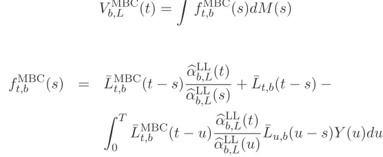
V_b,LMBC(t) =

Z

f_t,bMBC(s)dM(s)

where

f_t,bMBC(s) = L¯MBC_t,b (t−s)αb LL

b,L(t)

b

αLL

b,L(s)

+ ¯Lt,b(t−s)−

Z T

0 ¯

LMBC_t,b (t−u)αb LL

b,L(t)

b

α_b,LLL(u)L¯u,b(u−s)Y(u)du

and

B_b,LMBC(t) = B_b,LLL(t) +

Z

¯

LMBC_t,b (t−s)α_bLL_b,L(t)α_bLL_b,L(s) −1B_b,LLL(s)Y(s)ds

=

Z

¯

LMBC_t,b (t−s)α_bLL_b,L(t){βb,L(t)−βb,L(s)}Y(s)ds,

with βb,L(s) ={αbLLb,L(s)}−1Bb,LLL(s), where Bb,LLL and Vb,LLL are the stable and variable terms

for the local linear estimator given in (15) and (16), respectively.

Using the above decomposition and derivations similar to the local linear case we can expand the integrated squared error of the multiplicative bias corrected estimator. In Lemma 7 in the Supplementary Material we show that, under some regularity assumptions, ∆MBC

L (b) is asymptotically equivalent to

M_LMBC(b) =b8µ2( ¯L ∗₎4

16

Z

h(t)2γ(t)w(t)dt+ (nb)−1R(Γ_L¯∗)

Z

α(t)w(t)dt,

with h(t) = α(t){α′′(t)/α(t)}′′. From this approximation a deterministic optimal band-width for the multiplicative bias corrected estimator with kernel Lis defined as

bMBC_MISE,L=C₀MBC_,L n−1/9; C₀MBC_,L =

(

R(Γ_L¯∗)

R

α(t)w(t)dt µ2( ¯L∗)4

2

R

h(t)2_γ(t)w(t)dt

)1/9

, (18)

where Γ_L¯∗(u) = 2 ¯L∗(u)−L¯∗(u)∗L¯∗(u) is the kernel obtained by twicing the equivalent

kernel, ¯L∗, given in (7).

The following theorem states the asymptotic normality of the three bandwidth estimates, as well as the minimizer of the mean integrated squared error, for the multiplicative bias corrected hazard estimator with kernel K. The proof is provided in the Supplementary Material.

Theorem 3 Under assumptions A1, A2’ and A3’, the bandwidth selectors bbMBC_BO,K, bbMBC_DO,K,

bbMBC_CV,K, andbbMBC_MISE,K satisfy

n3/18bbMBC_BO,K −bbMBC_ISE,K −→N 0, S₂MBC+S₁MBCΨMBC_BO,K

n3/18bbMBC_DO,K −bbMBC_ISE,K −→N 0, S₂MBC+S₁MBCΨMBC_DO,K

n3/18bbMBC_CV,K −bbMBC_ISE,K −→N 0, S₂MBC+S₁MBCΨMBC_CV,K

n3/18bbMBC_MISE,K −bbMBC_ISE,K −→N 0, S₂MBC+S₁MBCΨMBC_MISE,K

where

S₁MBC = 2

1/3

92

R(ΓK)−5/6Rα(t)2w(t)2 dt

µ2(K)4/3R h(t)2γ(t)w(t) dt 1/3R α(t)w(t) dt 5/3

,

S₂MBC = 2

10/3

92

R(ΓK)−2/3R h(t)2γ(t)w(t)2α(t) dt

µ2(K)4/3R α(t)w(t) dt 2/3R h(t)2γ(t)w(t) dt 4/3

with

ΨMBC_BO,K = ΨMBC_DO,K =

Z _R(Γ

K) R(Γ_L¯∗)

HΓ_L¯_∗ −GΓ_L¯_∗

(ρMBCu)−HΓK(u)

2

du,

ΨMBC_CV,K =

Z

{GΓK(u)} 2 _du,

ΨMBC_MISE,K =

Z

{HΓK(u)} 2

du.

where the functionsGL(·)andHL(·)are defined as in Theorem 1, withL= ΓK andL= Γ_L¯∗,

defined above.

Remark 4 The result above shows that all bandwidth selectors have similar asymptotics

with the only difference of the factor ΨMBC

·,K . A similar conclusion was derived for the local linear estimator. The three last columns of Table 1 show the value of this factor for three common choices of K. As for the local linear estimator we have calculated the ratio SMBC

1 /S2MBC for a particular hazard model, the results are shown in Appendix B.2. In this

case the term S₁MBC, relative to the term S₂MBC, is negligible when exposure time goes to zero, but dominates completely (infinite times bigger) when exposure time goes to infinity.

6. Applications

6.1 Old-age mortality

Our first application is on fitting hazard mortality curves for old-age population. We con-sider mortality data of women in Iceland in the calendar year 2006, with ages from 40 to 110. The same data were considered by G´amiz et al. (2016) and are available in the

DOvalidation_{R-package (G´amiz et al., 2017). This package provides also functions}

imple-menting the hazard estimators and the bandwidth selection methods described above. The data were obtained from the Human Mortality Database and consist of aggregated yearly occurrences and exposures. G´amiz et al. (2016) showed that estimating the hazard from these data is challenge at the oldest ages. The lack of exposure at the right end and the few observed deaths induce a marked boundary effect precisely in the area of interest, the old ages. For these data we have calculated the two hazard estimators described in this paper, local linear and its multiplicative bias correction, using three bandwidth selectors: cross-validation, double one-sided cross-validation and the new best one-sided cross-validation. The cross-validation scores involved in these methods have been defined using a weighting function such thatw(s)Y(s)≡1, so all points in the time interval where the hazard function is estimated are evaluated with the same weight. This is different from G´amiz et al. (2016) where the weighting function was chosen so only areas where the exposure is significant contribute to the criteria. Notice that this makes an important difference in this data set where the end of the time interval comprises almost no exposure.

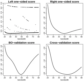
Figure 1: Mortality data: bandwidth selection scores with multiplicative bias corrected hazard estimator.

20 30 40 50 60 70 80

0.5

1.0

1.5

2.0

2.5

3.0

3.5 Left one−sided score

bandwidth

20 30 40 50 60 70 80

−16

−14

−12

−10

−8

−6

Right one−sided score

bandwidth

20 30 40 50 60 70 80

−18

−17

−16

−15

−14

−13

−12

BO−validation score

bandwidth

20 30 40 50 60 70 80

−18

−16

−14

−12

−10

Cross−validation score

bandwidth

hazard estimators. Therefore the average DO-validated bandwidth becomes unreliable, even though the obtained values seem to be sensible (bbDO = 27.3 for the local linear estimator andbbDO= 40 for its multiplicative bias correction). On the other hand the best one-sided cross-validation method shows a clear minimum in both cases and, as expected, it moves close to the one-sided cross-validated bandwidth that is working fine (the right side in this case). Best one-sided cross-validation in this case has been calculated using the exposure process, that is, for each timetwe use the functionξE

b (t) given in (11). However the results

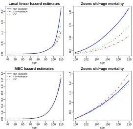
are quite similar using the occurrence process instead. Figure 2 shows the resulting hazard estimates from each method and type of hazard estimate. Note from these plots that the multiplicative bias corrected hazard is more robust to the bandwidth choice than the local linear. Also the new best one-sided cross-validation method seems to provide a reasonable estimate for old-age mortality in both cases.

6.2 Prediction of outstanding liabilities in non-life insurance

Figure 2: Comparison of hazard estimates from female mortality data in Iceland.

40 50 60 70 80 90 100 110

0.0

0.5

1.0

1.5

2.0

Local linear hazard estimates

age

BO−validation DO−validation CV

100 102 104 106 108 110

0.5

1.0

1.5

2.0

Zoom: old−age mortality

age

40 50 60 70 80 90 100 110

0.0

0.2

0.4

0.6

0.8

1.0

1.2

1.4

MBC hazard estimates

age

BO−validation DO−validation CV

100 102 104 106 108 110

0.6

0.8

1.0

1.2

1.4

Zoom: old−age mortality

age

Mart´ınez-Miranda et al. (2013) for a detailed background of this problem). Here we analyse a data set of reported and outstanding claims from a motor business in UK. The same data set was previously considered by Mart´ınez-Miranda et al. (2013) and consists of n= 1558 large claims reported between January 1990 and March 2012. From a statistical perspective the data could be described as a sample {(X1, Z1), . . . ,(Xn, Zn)}, where Xi denotes the

underwriting date of the ith claim, and Zi the corresponding reporting delay, this is, the

time between the underwriting date and the reporting date of the claim. The sample is right truncated since it can be observed only those claims for which the underwriting time plus the reporting delay is not greater than the calendar time of data collection. Hence data exist on a triangle withXi+Zi ≤31 March 2012, andXi+Zi represents the calendar time. The aim

is to forecast the mass of the unobserved, future triangle, where Xi+Zi >31 March 2012,

which corresponds to the number of claims underwritten in the past which have not been reported yet. The problem is formulated assuming that the maximum reporting delay is 267 months, in the actuarial literature this assumption is described as the triangle is fully run off. Another challenge of the data set for this problem is that the data are only available in an aggregated way. This is a common feature of this kind of data in the reserving departments of the insurance companies. This means that the available observations are counts living in a triangle of dimension 267×267. Specifically for our data set the triangle has entriesNx,z=Pn_i=1I(Xi =x, Zi =z), withx, z∈ {1, . . . ,267}, describing the number

Mart´ınez-Miranda et al. (2013) showed that a multiplicative structured density model,

f(x, z) =f1(x)f2(z), can be used to forecast the claims where the componentsf1 andf2are the underwriting time density and the reporting time density, respectively. The assumption of a multiplicative density means that the reporting delay does not depend on the under-writing date. Using the counting process formulation considered in this paper, Hiabu et al. (2016) solved the forecasting problem estimating the two density components using a time-reversal approach. Data are transformed to the time reversed scale so the right-truncation problem is replaced by the more tractable left-truncation. Using the same time-reversal approach, we now use the hazard estimation methods presented in the previous sections to estimate the backward hazard functions corresponding to the two components, under-writing (α1) and reporting delay (α2). From these hazard estimates the density component estimates can be derived multiplying by respective estimators of the survival functions.

From the above description we solve the forecasting problem considering both local linear hazard estimator and its multiplicative bias correction. For each hazard component, the bandwidth parameters for these estimators have been estimated using cross-validation, double one-sided cross-validation and best one-sided cross-validation. In the three cases we use weighting functions for the involved cross-validation scores that are appropriate for the forecasting problem. Specifically, following the discussion in Hiabu et al. (2016), to estimate

α1 we consider weights w1(t) =Sb12(t)

n

1−Sb2(t)

o2

/Y1(t), whereSb1 and Sb2 are estimators of the survival functions of each component (underwriting time and the reporting time delay) on the reversed time scale; andY1(t) is the risk process for the first component. In a similar way we define the weights to estimateα2. As in the mortality study best one-sided cross-validation has been calculated using the exposure process.

compo-Table 2: Forecasts of the number of claims to be reported in the future calendar years.

Year CLM LL-CV LL-DO LL-BO MBC-CV MBC-DO MBC-BO 2012 99.95 76.85 77.98 77.95 80.55 81.75 81.76 2013 97.23 75.06 75.52 76.86 81.18 75.82 81.68 2014 74.32 58.75 59.05 60.04 62.23 58.89 62.88 2015 49.18 38.88 39.06 39.44 40.31 38.81 41.20 2016 24.52 19.42 19.50 19.66 20.01 19.34 20.44 2017 11.61 9.35 9.39 9.44 9.60 9.45 9.76 2018 6.21 5.07 5.06 5.09 5.15 4.99 5.27 2019 3.24 2.54 2.53 2.52 2.52 2.53 2.61 2020 1.36 1.25 1.23 1.23 1.23 1.18 1.22 2021 0.99 1.03 1.02 1.02 0.99 0.95 0.95 2022 1.11 0.85 0.84 0.85 0.87 0.83 0.88 2023 1.06 0.71 0.71 0.73 0.81 0.80 0.85 2024 1.20 0.81 0.81 0.84 0.93 0.90 0.94 2025 1.14 0.91 0.92 0.95 0.97 0.93 0.94 >2025 1.94 1.59 1.59 1.61 1.51 1.48 1.55 Total 375.07 293.07 295.20 298.23 308.86 298.69 312.92

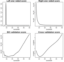
nent, exhibiting several local minima. For the reporting delay component the score function continues decreasing as the value of the bandwidth increases, so it reaches the minimum at the upper limit of the search interval of bandwidths. The left one-sided score behaves more reasonably for the underwriting component but again breaks down for the reporting de-lay component. This means that one shouldn’t trust the double one-sided cross-validation bandwidth derived from these two one-sided criteria, even though the derived estimates in this case turned to be reasonable values, bbDO = 55.8 for the underwriting time, and

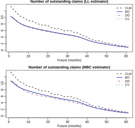
bbDO= 31.6 for the delay. On the contrary, the new best one-sided cross-validation method provides bandwidth estimates ofbbBO = 43.4 for the underwriting time andbbBO = 11.8 for the delay, exhibiting well-behaved minimization scores as shown in Figure 4. Regarding to the cross-validation method it exhibits a rather flat score in the underwriting compo-nent leading to the large bandwidth estimate of bbCV = 63.5, and a value of bbCV = 11.6 for the delay that is close to the best one-sided cross-validated bandwidth. The impact of the cross-validated bandwidths on the forecasts is moderated, about 309 predicted claims compared to the 313 from best one-sided cross-validation. We have performed the same inspection with the local linear estimators. These plots can be seen in the Supplementary Material. The picture is again quite similar showing a poor performance of double one-sided cross-validation, however the impact on the forecasts in this case is not substantial. The total number predicted from cross-validation is about 293, compared to 295 from double one-sided cross-validation and 298 for best one-sided cross-validation.

7. Finite sample performance

Figure 3: Number of outstanding claims forecast using the local linear estimator and its multiplicative bias correction.

0 10 20 30 40 50 60

0

2

4

6

8

10

Number of outstanding claims (LL estimator)

Future (months)

CLM BO DO CV

0 10 20 30 40 50 60

0

2

4

6

8

10

Number of outstanding claims (MBC estimator)

Future (months)

Figure 4: Underwriting component: bandwidth selection scores with multiplicative bias corrected hazard estimator.

20 30 40 50 60 70

−0.00084

−0.00080

−0.00076

−0.00072

Left one−sided score

bandwidth

20 30 40 50 60 70

2e−04

4e−04

6e−04

8e−04

Right one−sided score

bandwidth

20 30 40 50 60 70

−0.00084

−0.00080

BO−validation score

bandwidth

20 30 40 50 60 70

−0.00084

−0.00082

−0.00080

−0.00078

Cross−validation score

Figure 5: Reporting delay component: bandwidth selection scores with multiplicative bias corrected estimator.

10 20 30 40 50

0.0

0.1

0.2

0.3

0.4

0.5

Left one−sided score

bandwidth

10 20 30 40 50

0e+00

5e−04

1e−03

Right one−sided score

bandwidth

10 20 30 40 50

0e+00

5e−04

1e−03

BO−validation score

bandwidth

10 20 30 40 50

−0.00051

−0.00049

Cross−validation score

Supplementary Material). The first four models consist of mixtures of Beta densities. Model 5 shows an exponential increase common in hazard mortality rates as those described in the first case study of Section 6. From each model we have simulated samples with three different sample sizes and two sampling schemes, right censoring with and without left truncation. For models 1 to 4 we have considered sample sizes n = 100,1000,10000, and for model 5, n = 50000,75000,100000. The number of Monte Carlo replications for each case has been always 500. We use the same mechanism to simulate data as in G´amiz et al. (2016). It generates data in aggregated form (number of occurrences and exposure) for an equally-spaced grid of size R defined on the time interval, and always produces right censored samples. For models 1 to 4 the time interval is (0,1) and we have defined the grid length with δR = 1/(R+ 1). For model 5 time lies in the interval (40,110) and we

have defined the grid length withδR= 70/(R+ 1). The grid size has been chosen equal to R= 500 in both cases. We shall denote the grid points bytr (r= 1, . . . , R). In the case of

samples without left truncation, for a sample ofnindividuals, the number of occurrences at timetr, denoted asOr, have been generated from the binomial distributionBi{Yr, α(tr)δR},

forr = 1, . . . , R. HereYr denotes the size of the risk set at the beginning of therth interval

of the grid. The total number of simulated occurrences does not sum to n. Some of the simulated individuals are finally right censored, because they are still at risk at the end of the interval. Therefore our simulated sample are right censored and the censoring rates are around 20–30% for all models. When adding left truncation, independent truncation times are generated from the Uniform distribution.

From the simulated aggregated data we have calculated the local linear hazard estima-tor and its multiplicative bias correction using the sextic kernel: K(x) = 3003/2048(1−

x2)6I(−1< x < 1), as in the two data analyses above. For each hazard estimator we have compared the best one-sided cross-validated bandwidth with cross-validation and double one-sided cross-validation. The performance of the bandwidth estimates have been anal-ysed with respect to the (Monte Carlo approximated) mean integrated squared error of the resulting kernel hazard estimator. We shall refer to this performance measure as empirical MISE, denoted as m1(bb), for each bandwidth estimatebb. As benchmarks in our analysis we have considered two infeasible optimal bandwidths: the bandwidth minimizing the inte-grated squared error criterion,bbISE, and the bandwidth minimizing the empirical MISE. To compute all bandwidth estimates we have considered grids of 100 equally spaced bandwidth values chosen aroundbbISE, for each model and sample size. All criteria have been defined using a weighting function such that w(s)Y(s)≡1, so all points in the time interval where the hazard function is estimated are evaluated with the same weight. As we pointed out in our first case study this is different from G´amiz et al. (2016), and it makes an important difference in models such as Model 5 where the end of the time interval comprises almost no exposure.

Table 3 summarizes the simulation results in the case of samples with right censoring and left truncation. In this table bandwidth estimates are compared according to measure

m1. For convenience we report a relative measure to indicate when best one-sided cross-validation outperforms cross-cross-validation. The relative measure is defined as:

Rerr(BO) =nm1(bbCV)−m1(bbISE)

o

/nm1(bbBO)−m1(bbISE)

o

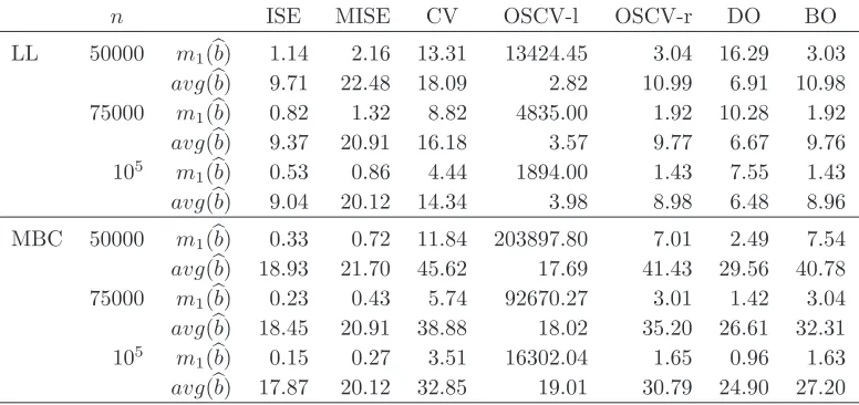
With this definition values ofRerr(BO) above 1 indicate that best one-sided cross-validation outperforms cross-validation. An analogous relative measure, Rerr(DO), has been defined for double one-sided cross-validation. Notice that Rerr(BO) greater than Rerr(DO) indi-cates that best one-sided cross-validation outperforms double one-sided cross-validation. An overall view of the numbers in the table confirms that best one-sided cross-validation for the multiplicative hazard estimator always outperforms cross-validation, exhibitingRerr(BO) values above 1, and double one-sided cross-validation for all models except for few cases, where double one-sided cross-validation provides slightly lower empirical MISE values. The results for the local linear estimator show that double one-sided cross-validation and best one-sided validation behave quite similarly, both outperforming in general cross-validation. The case of samples without left truncation is shown in Table 4. It brings similar conclusions though in this case best one-sided cross-validation is beaten by double one-sided cross-validation for Model 5. This case deserves a deeper analysis and it is shown in Table 5. In this table we have shown the empirical MISE defined above and denoted by

m1(bb), for each bandwidth estimatebb, as well as the average of the bandwidth estimates for all the samples (avg(bb)), and we have included the left and right one-sided cross-validated bandwidths, from which double one-sided cross-validation is derived. From these results we can clearly see that the left one-sided bandwidth completely breaks down, for all sample sizes and both hazard estimators, while the right side behaves well (notice the large values of the empirical MISE for the left one-sided bandwidth in contrast with those values for the right one-sided bandwidth). The average of the left and right one-sided bandwidths (which double one-sided cross-validation performs) seems to be hiding the problem of the left side, and sometimes it even provides quite reasonable values. Notice that the double one-sided bandwidths are on average closer to the best ISE-optimal bandwidths than the best one-sided cross-validation for the multiplicative bias corrected estimator. However this happens because the double one-sided bandwidth is the average of a small left one-sided bandwidth and a large right one-sided bandwidth. On the other hand best one-sided cross-validation is behaving as the best of the two sides, as we would expect. A similar picture can be seen when analysing the behaviour of double one-sided cross-validation for Model 4 in the case of truncated samples (the full simulation results are provided in the Supplementary Material). In summary, the simulation results indicate that best-one sided cross-validation and double one-sided cross-validation do better than one-sided cross-validation (that sometimes breaks down) and standard cross-validation. However, it is not always which one is the better of best one-sided cross-validation or double one-sided cross-validation. We suggest to try out both best one-sided and double one-sided cross-validation in any empirical study.

8. Discussion

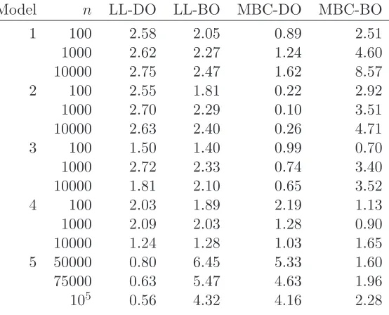
Table 3: Simulation results for datasets with right censoring and left truncation. Hazard estimators and bandwidth selectors are compared by the relative measureRerr(·) defined in (19).

Model n LL-DO LL-BO MBC-DO MBC-BO 1 100 1.55 1.25 1.47 1.79 1000 2.32 2.00 0.97 2.88 10000 1.90 1.71 1.82 3.30 2 100 2.28 2.04 0.46 2.47 1000 2.42 1.99 0.15 3.66 10000 2.18 1.84 0.34 3.81 3 100 1.86 1.74 1.47 1.27 1000 0.96 0.99 0.82 1.19 10000 2.20 2.07 2.12 3.50 4 100 0.08 1.12 2.13 0.92 1000 2.51 1.91 2.30 1.08 10000 2.17 1.83 3.76 2.62 5 50000 1.62 1.70 1.77 2.09 75000 2.04 2.18 1.41 2.31 105 _{1.68 1.73 1.07 1.90}

Table 4: Simulation results for datasets without left truncation. Hazard estimators and bandwidth selectors are compared by the relative measureRerr(·) defined in (19).

Table 5: Performance of double one-sided cross-validation in simulations. The empirical MISE (multiplied by 106_{), m}

1(bb), and the average bandwidth estimates, avg(bb), are shown for samples generated from Model 5 without left truncation.

n ISE MISE CV OSCV-l OSCV-r DO BO

LL 50000 m1(bb) 1.14 2.16 13.31 13424.45 3.04 16.29 3.03

avg(bb) 9.71 22.48 18.09 2.82 10.99 6.91 10.98 75000 m1(bb) 0.82 1.32 8.82 4835.00 1.92 10.28 1.92

avg(bb) 9.37 20.91 16.18 3.57 9.77 6.67 9.76 105

m1(bb) 0.53 0.86 4.44 1894.00 1.43 7.55 1.43

avg(bb) 9.04 20.12 14.34 3.98 8.98 6.48 8.96

MBC 50000 m1(bb) 0.33 0.72 11.84 203897.80 7.01 2.49 7.54

avg(bb) 18.93 21.70 45.62 17.69 41.43 29.56 40.78 75000 m1(bb) 0.23 0.43 5.74 92670.27 3.01 1.42 3.04

avg(bb) 18.45 20.91 38.88 18.02 35.20 26.61 32.31 105

m1(bb) 0.15 0.27 3.51 16302.04 1.65 0.96 1.63

avg(bb) 17.87 20.12 32.85 19.01 30.79 24.90 27.20

while the performance is vice versa when using the multiplicative kernel hazard estimation. The exception from this rule seems to be our finite sample study in Table 5 inspired by our real-life mortality data.

9. Conclusion

We have proposed a new bandwidth selection method for local linear hazard estimation and its multiplicative bias correction. Our proposal is called best one-sided cross-validation and consists of an improvement of the double one-sided cross-validation of G´amiz et al. (2016). Best one-sided validation solves the lack of stability of double one-sided cross-validation in practice via a local information principle.

Our empirical studies show that best one-sided cross-validation provides a good strat-egy for bandwidth selection for both local linear and multiplicative bias corrected hazard estimators. Best one-sided validation inherits the good properties of one-sided cross-validation while avoiding the stability problems that double one-sided cross-cross-validation some-times faces. The current algorithm is only about optimisation of statistical inference. How-ever, it could be also interesting to consider computational performance, see for example Kapotufe and Verma (2017).

Detailed mathematical theory at the level of Hall and Marron (1987) and G´amiz et al. (2016) is included. This type of theory is completely novel for the multiplicative bias corrected hazard estimators. Theory on best one-sided cross-validation introduced in this paper is of course also new for the local linear hazard estimator.

Acknowledgments

The authors are grateful for constructive comments from an anonymous Reviewer and the Associate Editor. This work has been partially supported by the Spanish Ministry of Economy and Competitiveness, through grant number MTM2016-76969P, which include support from the European Regional Development Fund (ERDF). The authors thank Centro de Servicios de Inform´atica y Redes de Comunicaciones (CSIRC), University of Granada, for providing the computing time.

Appendix A. Assumptions for asymptotic theory

Assumption A1. The kernels K and L are compactly supported (i.e. the support

is contained in [−CK, CK] for some constants CK >0). The kernels are continuous

on IR\{0} and have one-sided derivatives that are H¨older continuous onIR− ={x :

x < 0} and IR+ = {x : x > 0}, that is there exist constants c and d such that

|φ(x)−φ(y)| ≤c|x−y|d _{for x, y <0 orx, y > 0 withφ equal to K}′ _orL′_{. The}

left-and right-sided derivatives differ at most on a finite set. The kernelK is symmetric.

Assumption A2. For the expected exposure functionγ(t) =n−1E{Y(t)}it holds that

γ ∈C2([0, T]), that it is strictly positive for t∈[0, T], and that

sup

s∈[0,T]

|Y(s)/n−γ(s)| = oP(logn)−1 ,

sup

s,t∈[0,T],|t−s|≤CKb

|{Y(t)−Y(s)}/n− {γ(t)−γ(s)}| = oP

n

(nblogn)−1/2o,

AssumptionA2’. Same conditions as in assumption A2 but replacingoP(nblogn)−1/2

withoP(nb)−1

Assumption A3. It holds that α ∈ C2([0, T]), w ∈C1([0, T]). The second derivative of α is H¨older continuous with exponent d >0.

Assumption A3’. Same conditions as in assumption A3 but α ∈ C4([0, T]) and its fourth derivative is H¨older continuous.

Appendix B. Evaluation of the common variance terms

In Section 5 we compare bandwidth selectors by their asymptotic variances which are of the formS2+S1Ψ, where Ψ is a factor that differs among bandwidth selectors, while the terms

S1andS2are common for all of them. For both the local linear and the multiplicative biased corrected hazards, the factor Ψ only depends on the chosen kernels so we have evaluated it for some common choices in Table 1. The terms terms S1 and S2 however depend on the hazard function α, the exposure function γ and the weighting function w. Here we evaluate the ratio S1/S2 for the two hazard estimators, considering a specific choice for these functions. We consider a hazard function of the form α(t) =λ+cexp(βt), whereλ,

cand β are constants. This hazard specification characterizes the Gompertz-Makeham law of mortality, where the empirical magnitudes for the parameters β and c are about 0.085 and 3×1031_{, respectively. For the weighting function we consider the case w(t) ≡1, and} for the exposure function the caseγ(t) = 1{0≤t≤T}, forT >0.

B.1 Local linear estimator

For the local linear hazard estimators the termsS1 and S2 are given by

S₁LL = 1 25

R(K)−7/5R _α2_(t)w2_{(t) dt}

µ2(K)6/5R α′′(t)2γ(t)w(t)dt 3/5R α(t)w(t)dt 7/5

,

S₂LL = 4 25

R(K)−2/5R_α′′_(t)2_γ(t)w2_{(t)α(t) dt}

µ2(K)6/5R α(t)w(t) dt 2/5R α′′(t)2γ(t)w(t)dt 8/5

,

The ratio RLL_=SLL

1 /S2LL, forγ(t) = 1{0≤t≤T} and w(t)≡1, is given by

RLL = S LL 1

SLL 2

= 1

4R(K)

RT

0 α2(t) dt

RT

0 α′′(t)2 dt

RT

0 α(t) dt

RT

0 α′′(t)2α(t) dt

For the choice α(t) =λ+cexp(βt) the above integrals become

Z T

0

α(t) dt = c

β (exp(βT)−1) +λT

Z T

0

α(t)2 dt = c 2

2β (exp(2βT)−1) +λ

2_{T +}2λc

Z T

0

α′′(t)2 dt = c 2_β3

2 (exp(2βT)−1)

Z T

0

α′′(t)2α(t) dt = c 3_β3

3 (exp(3βT)−1) +

λc2_β3

2 (exp(2βT)−1)

We substitute these results in the expression of RLL _{and take limits forT → ∞. We only} look at the leading terms in the numerator and the denominator (that is exp(4βT)) and we get that RLL → 3/(16R(K)), as T → ∞. For the Epanechnikov kernels the limit is

5/16. Notice that the limit at zero is RLL → (4R(K))−1, which takes the value 5/12 for

the Epanechnikov kernel.

B.2 Multiplicative bias corrected estimator

For the multiplicative bias corrected estimator the terms are

S₁MBC = 2 1/3

92

R(ΓK)−5/6R α(t)2w(t)2 dt

µ2(K)4/3R h(t)2γ(t)w(t) dt 1/3R α(t)w(t) dt 5/3

,

S₂MBC = 2 10/3

92

R(ΓK)−2/3R h(t)2γ(t)w(t)2α(t) dt

µ2(K)4/3R α(t)w(t) dt 2/3R h(t)2γ(t)w(t)dt 4/3

,

whereh(t) =α(t)(α′′(t)/α(t))′′.

We compute the ratio RMBC =S₁MBC/S₂MBC for the same choice of γ and w as before. It yields to the following expression

RMBC= S MBC 1

SMBC 2

= 1

8R(ΓK)1/6

RT

0 α2(t) dt

RT

0 h(t)2 dt

RT

0 α(t) dt

RT

0 h(t)2α(t) dt

For the choiceα(t) =λ+cexp(βt) the calculations are as follows:

Z T

0

α(t) dt = c

β(exp(βT)−1) +λT

Z T

0

α(t)2 dt = c 2

2β(exp(2βT)−1) +λ

2_T+2λc

β (exp(βT)−1)

Z T

0

h2(t)dt =

Z λ+cexp(βT)

λ+c

cβ7λ2e βt

y4 (2λ−y)

2_dy=Z λ+cexp(βT)

λ+c

β7λy−λ

y4 (2λ−y) 2_dy

=

Z λ+cexp(βT)

λ+c

β7λ2

8

y3λ 2₋ 4

y4λ 3₋ 5

y2λ+ 1

y

dy

= β7λ2

4λ3

3y3 − 4λ2

y2 + 5

λ y + lny

y=λ+cexp(βT)

y=λ+c

Here

h(t) = α(t)

d2 dt2 α

′′_(t)/α(t)

=cβ4λ e tβ

(λ+cetβ₎2

λ−cetβ,

and we have made the change of variable y=α(t),dy=cβeβtdt=β(y−λ) dt. Similarly

Z T

0

h2(t)α(t) dt =

Z λ+cexp(βT)

λ+c

cβ7λ2e βt

y3(2λ−y)

2_dy=Z λ+cexp(βT)

λ+c

β7λy−λ

y3 (2λ−y) 2_dy

=

Z λ+cexp(βT)

λ+c

β7λ2

8

y2λ 2₋ 4

y3λ 3₋5

yλ+ 1

dy

= β7λ2

2λ3

y2 − 8λ2

y −5λln(y) +y

y=λ+cexp(βT)

y=λ+c

We then substitute the above results in the expression ofRMBCand take limits forT → ∞. To this goal we only look at the leading terms in the numerator and the denominator and we get thatRM BC→ ∞asT → ∞. And the ratio increases to∞as log(λ+cexp(βT)), this

is, at the linear rateβT. The limit forT →0 is (8R(ΓK))−1/6, which for the Epanechnikov

kernel is about 0.13.

References

Aalen, O. O. (1978). Non-parametric inference for a family of counting processes. Ann. Statist.,6, 701–726.

Andersen, P., Borgan, O., Gill, R. and Keiding, N. (1993). Statistical Models Based on Counting Processes. New York: Springer.

G´amiz, M. L., Mammen, E., Mart´ınez-Miranda, M. D. and Nielsen, J. P. (2016). Double one-sided cross-validation of local linear hazards. J. Royal Statist. Soc. B,78, 755–779.

G´amiz, M. L., Mammen, E., Mart´ınez-Miranda, M. D. and Nielsen, J. P. (2017).

DOvalidation_{: Kernel Hazard Estimation with Best One-Sided and Double One-Sided} Cross-Validation. R package version 1.1.0.

G´amiz, M. L., Mart´ınez-Miranda, M. D. and Nielsen, J. P. (2013a). Smoothing survival densities in practice. Comput. Statist. Data Anal.,58, 368–382.

G´amiz, M. L., Janys, L., Mart´ınez-Miranda, M. D. and Nielsen, J. P. (2013b). Bandwidth selection in marker dependent kernel hazard estimation. Comput. Statist. Data Anal.,

68, 155–169.

Hall, P. and Johnstone, I. (1992). Empirical Functionals and Efficient Smoothing Parameter Selection. J. Royal Statist. Soc. B,54(2), 475–530.

Hart, J. D. and Yi, S. (1998) One-Sided Cross-Validation.J. Am. Statist. Ass.,93, 620–631.

Hiabu, M., Mammen, E., Mart´ınez-Miranda, M. D. and Nielsen, J. P. (2016) In-sample forecasting with local linear survival densities. Biometrika,103, 843–859.

Jones, M. C., Linton, O. B. and Nielsen, J. P. (1995). A simple bias reduction method for density estimation. Biometrika,82, 327–38.

Jones, M. C. and Signorini, D. F. (1997). A comparison of higher-order bias kernel density estimators. J. Am. Statist. Ass.,92, 1063–1073.

Kapotufe, S. and Verma, N. (2017). Time-Accuracy Tradeoffs in Kernel Prediction: Con-trolling Prediction Quality. J. Mach. Learn. Res.,18, 1–29.

Mammen, E., Mart´ınez-Miranda, M. D., Nielsen, J. P. and Sperlich, S. (2011). Do-validation for kernel density estimation. J. Am. Statist. Ass.,106, 651–660.

Mammen, E., Mart´ınez-Miranda, M. D., Nielsen, J. P. and Sperlich, S. (2014). Further theoretical and practical insight to the do-validated bandwidth selector.J. Korean Statist. Soc.,43, 355–365.

Mammen, E. and Nielsen, J. P. (2007). A general approach to the predictability issue in survival analysis with applications. Biometrika,94, 873–892.

Mart´ınez-Miranda, M. D., Nielsen, J. P., Sperlich, S. and Verrall, R. (2013). Continuous Chain Ladder: Reformulating and generalizing a classical insurance problem. Expert Syst. Appl.,40(14), 5588–5603.

Mu˜noz, I. D. and van der Laan, M. J. (2012). Super Learner Based Conditional Density Estimation with Application to Marginal Structural Models. Int. J. Biostat.,7(1), article 38.

Nielsen, J. P. (1998). Multiplicative bias correction in kernel hazard estimation. Scand. J. Statist.,25, 541–553.

Nielsen, J. P. and Tanggaard, C. (2001). Boundary and bias correction in kernel hazard estimation. Scand. J. Statist.,28, 675–698.

Savchuk, O. Y., Hart, J. D., Sheather S. J. (2010). Indirect crossvalidation for density estimation. J. Am. Statist. Ass.,105, 415–423.

Sheather, S. J. and Jones, M. C. (1991). A reliable data-based bandwidth selection method for kernel density estimation. J. Royal Statist. Soc. B,53, 683–690.