Direct transcription of optimal control problems with finite elements on Bernstein basis

Direct Transcription of Optimal Control Problems with Finite

Elements on Bernstein Basis

Lorenzo A. Ricciardi∗, Massimiliano Vasile† University of Strathclyde, Glasgow, United Kingdom, G1 1XJ

The paper introduces the use of Bernstein polynomials as a basis for the direct transcription

of optimal control problems with Finite Elements in Time. Two key properties of this new

transcription approach are demonstrated in this paper: Bernstein bases return smooth control

profiles with no oscillations near discontinuities or abrupt changes of the control law, and

for convex feasible sets, the polynomial representation of both states and controls remains

within the feasible set for all times. The latter property is demonstrated theoretically and

experimentally. A simple but representative example is used to illustrate these properties and

compare the new scheme against a more common way to transcribe optimal control problems

with Finite Elements in Time.

Nomenclature

ψ _{Boundary constraints}

∆T Length of finite element

F Differential equations of motion

g Algebraic constraints

u _{Control vector}

us j Weights for the polynomials of the controls

w Test functions

ws j Weights for the polynomials of the test functions

x _{State vector}

x₀ Initial conditions

xf Final conditions

xs j Weights for the polynomials of the states

σk Gauss integration weights

τ Adimensional time

τk Gauss integration nodes

Bν,n Generic Bernstein polynomial of degreen

D Time domain

fs j Generic polynomial basis for the states

gs j Generic polynomial basis for the controls

hs j Generic polynomial basis for the test functions

J Objective function ∗

Ph.D. Candidate, Aerospace Centre of Excellence, Mechanical & Aerospace Engineering, 75 Montrose Street, G1 1XJ, Glasgow, AIAA Student Member.

†

l Order of the polynomials for the states

m Order of the polynomials for the controls

N Number of discretisation elements

q Number of integration nodes

t Time

t₀ Initial time

tf Final time

I. Introduction

O

ptimal control problems appear almost everywhere in modern engineering: from chemical reactions engineering

and drug dosage delivery, to robotics, to aeronautical and space vehicle trajectory optimisation, just to name a

few. Even if the theory of optimal control is very mature, obtaining a solution for these problems is still challenging,

especially for highly non-linear problems where the only possibility is to employ numerical techniques.

It is customary to classify numerical methods for the solution of open loop optimal control problems in indirect and direct

methods. The former analytically derive the necessary conditions for local optimality [1], while the latter transcribe the

original infinite dimensional problem into a finite dimensional problem, and solve the resulting NLP problem. The

transcription process generally makes use of an appropriate set of polynomials to represent states, controls or both.

Direct Finite Elements in Time (DFET) is a direct transcription method to solve optimal control problems and was

initially proposed by Vasile and Finzi [2] in 2000. Finite Elements in Time (FET) for the indirect solution of optimal

control problems were initially proposed by Hodges and Bless [3], and during the late 1990s evolved to the discontinuous

version. As pointed out by Bottasso and Ragazzi [4], FET for the forward integration of ordinary differential equations

are equivalent to some classes of implicit Runge-Kutta integration schemes, can be extended to arbitrary high-order, are

very robust and allow full h-p adaptivity. In the past decade, direct transcription with FET on spectral bases has been

successfully used to solve a range of difficult problems: from the design of low-thrust multi-gravity assist trajectories to

Mercury [5] and the Sun [6], to the design of weak stability boundary transfers to the Moon, low-thrust transfers in the

restricted three body problem and optimal landing trajectories to the Moon [2]. More recently they have been used to

perform multi-objective optimal control of spacecraft [7, 8], ascent trajectories of launchers [9], or abort trajectories of

reusable launch vehicles [10].

Although DFET were proven to be a valid technique to solve difficult optimal control problems, when the solution

presents very sharp variations in states and controls, like bang-bang control profiles, the polynomial representation of

states and controls can display undesired oscillations exceeding the bounds (also known as Gibbs phenomenon), even if

the nodal solution is correct. Although, h-p adaptivity strategies can be used, as proposed in [11], still oscillations can

remain regardless of the choice of the nodal values.

This is undesirable in a number of cases. Although the polynomial representation of states and controls is generally

solution at any other instant of time. Thus it cannot be used as guidance law. Furthermore, if different polynomial

orders or collocation points are used for states and controls, one could end up evaluating the polynomials at points

affected by the Gibbs phenomenon.

Also, one might want to evaluate some derived quantities at arbitrary points along the solution. Values coming from

those spurious oscillations that are outside the boundaries of states and controls could lead to numerical exceptions. A

regular behaviour in between two collocation nodes allows for a better re-integrability of the control law. Moreover

h-p adaptive techniques are iterative procedures which take a given solution, re-evaluate it on a more refined grid and

re-optimise it on this new grid. The re-evaluation on the more refined grid requires the evaluation of the solution at time

instants that are different from the nodal values. Thus, the resulting initial solution defined over the new grid could be

out of bounds, with resulting numerical difficulties or need for ad hoc procedures. All these problems could be solved

with a linear interpolation of the nodal solution for the controls, but a linear interpolation would be inconsistent if a

higher order polynomial representation was used to obtain the solution.

This paper proposes the use of Bernstein polynomials, for the DFET transcription method, instead of the commonly

used Lagrange interpolation on spectral bases. The use of Bernstein polynomials guarantees that the representation of

states and controls remains within the feasible set over the whole time domain and not only at the collocation nodes and

avoids the Gibbs phenomenon at points of jump discontinuity [12] or sharp slope variations. The paper will provide a

quantification of the computational cost of the use of both Lagrangeand Bernstein bases, for comparable accuracy. Two

metrics will be used: the sparsity pattern of the Jacobian of the constraints of the resulting NLP problem and the number

of iterations required to converge to the desired feasibility and optimality of the NLP solution. The computational cost

will be measured for an increasing order of the polynomials (p-refinement), at constant number of finite elements, and

for an increasing number of elements (h-refinement), at constant order of the polynomials. Two cases will be considered:

one with no path constraints but a sharp change in the control profile and one with a path constraint on one state variable.

Linear combinations of Bernstein polynomials generate the so called Bezier curves. The use of Bezier curves to

solve optimal control problems can be found in the work of Rogalsky [13] who solved optimal control problems with

linear dynamics, using Differential Evolution and Bezier curves to represent the control profile. He noted that the

resulting curves always lie in the convex hull of the control points and never present undesirable oscillations away from

its defining control points. Thus, Bézier curves could be used to parameterize smooth, non-oscillatory functions, with

minimal epistasis, using only a few parameters. In [14, 15], Gomanjani et al. used Bezier curves in the analytical

solution of some optimal control problems, with linear dynamics, because they led to a simpler symbolic manipulations,

while Darehmiraki et al. in [16] proposed the use of Bernstein polynomials with a weighted residual methods to solve

distributed optimal control problems. Similarly Mirkov and Rasuo in [17] proposed the use of Bernstein polynomials

to solve Elliptic Boundary value problems in a collocation method, while Bhatti and Bracken [18] proposed the use

with continuous solutions, collocation methods based on Bernstein polynomials had an exponential convergence rate

though slower than pseudo-spectral and Chebyshev collocation schemes. Finally Farouki and Rajan [19] showed that

the numerical conditioning of polynomials using Bernstein form is particularly stable under finite precision arithmetic.

It is interesting to note that only a few researchers exploited the convex hull and variation diminishing properties of

Bezier curves for optimal control problems. These properties are instead the main reason for this work. Here we show

that by choosing Bernstein polynomials as a basis for the parameterisation of states and controls, one can generate

solutions that display the aforementioned properties. Moreover, differently from previous works, Bernstein polynomials

are here used to solve general nonlinear optimal control problems. This work also includes a theorem that provides

some necessary conditions for the satisfaction of general path constraints, provided that the feasible region is convex and

states and controls are described by Bezier curves. Finally, the main contribution of this paper is to show the benefit of

using Bernstein basis, within the DFET transcription framework, when the solution has sharp variations in the control

law or simple path constraints.

II. Direct Transcription with Finite Elements in Time

A generic optimal control problem can be formulated as [1, 11, 20]:

min

u∈UJ=minu∈Uφ x(t0),x(tf),t0,tf ₊∫tf

t0

L(x(t),u(t),t)dt

s.t.

Û

x=F(x(t),u(t),t)

g(x(t),u(t),t) ≤₀

ψ x(t₀),x(tf),t0,tf

≤0

t∈ [t₀,tf]

(1)

where the scalartis time, the functionsx(t):[t0,tf] →Rnare the state vector, the functionsu(t):[t0,tf] →Rpare the control vector andJis the sum of a boundary state cost functionψ :Rn×Rp×R2 →Rand of the integral of a running cost functionL:Rn×Rp× [t0,tf] →R. The functionsx(t)belong to the Sobolev spaceW1,∞while the functionsu(t)belong toL∞.The vector fields that appear in the dynamic, path and boundary constraints, respectively,

areF:Rn×Rp× [t0,tf] −→Rn,g:Rn×Rp× [t0,tf] −→Rsandψ:R2n+2 −→Rq.

A. Problem Transcription with DFET

In this section we briefly recall how the transcription method based on Finite Elements in Time works. Following

integrated by parts leading to,

∫ tf

t₀

Û

w(t)Tx(t)+w(t)TF(x(t),u(t),t)dt−wT_fxb_f +wT₀xb₀ =0 (2)

wherew(t)are the generalised weight functions that must assume a value of 0 on either bound andxb are the boundary

values of the states, that may be either imposed or free. Note that, in this bi-discontinuous formulation, the value ofx(t)

at the boundaries does not coincide with either withxbf orx b

0. As remarked by Bottasso in [21], the weak form 2 of the ODEsxÛ =F(x(t),u(t),t)is a mathematically correct formulation even whenF(x(t),u(t),t)is not continuous or

differentiable.

Let the time domainDbe decomposed intoNfinite elements such that

D= N Ø

j=1

Dj(tj−₁,tj) (3)

and parametrise, over eachDj, the states, controls and weight functions as

xj(t)= l Õ

s=0

fs j(t)xs j (4a)

uj(t)= m Õ

s=0

gs j(t)us j (4b)

wj(t)= l+1 Õ

s=0

hs j(t)ws j (4c)

where the functionsxj,uj,wj are defined over each finite elementDj, the functions fs j(t),gs j(t)andhs j(t)are chosen

among the space of polynomials of degreel,mandl+1 respectively, and the vectorsxs j,us j,ws jare weights given to

each polynomial in each element. The polynomialshs jhave to assume a value of 0 on either the left or the right bound

of the element. It is practical to define eachDj over the normalised interval[−1,1]through the transformation,

τ=2

t−tj−tj−1 2

tj −tj−₁ (5)

This way the domain of the basis function is constant and irrespective of the size of the element and also overlaps

with the interval of the Gauss nodes that will be employed for the integration of the dynamics. Substituting the definitions

of the polynomials into the objective functions and integrating with Gauss quadrature formulas withqnodes leads to

˜

J=φ(xb₀,xb_f,t₀,tf)+ N Õ j=1 q Õ k=1

σkL(xj(τk),uj(τk), τk) ∆t

and for the variational constraints leads for every element jto the system q Õ k=1 σk Û

wj(τk)Txj(τk)+wj(τk)TFj(τk) ∆t

2

−wj(1)Txbj +wj(−1)Txbj−1=0 (7)

whereτk andσk are the Gauss nodes and weights,Fj(τk)is the shorthand notation forF xj(τk),uj(τk), τk, andxbj and

xb_j−

1denote the boundary values of elementjatt=tjandt=tj−1respectively. In previous implementations of DFET, algebraic constraints were evaluated at the Gauss integration nodes, but in the following we will propose a different

choice. DFET transcription is rather flexible, because it allows one to parameterise states and controls with any basis,

and these bases could also be different for every variable and element. Similarly it is possible to employ several choices

for the type and number of quadrature nodes. In the following some of this flexibility will be exploited to derive a new

scheme with unique characteristics.

B. Choice of Basis Functions

In the DFET literature, the basis is typically generated through a Lagrange interpolation on the quadrature nodes,

usually either Gauss-Legendre or Gauss-Lobatto:

fs j(τ)= l Ö

k=0,k,s

τ−τ_k τs−τk

, gs j(τ)= m Ö

k=0,k,s

τ−τ_k τs−τk

, hs j(τ)= l+1 Ö

k=0,k,s

τ−τ_k

τs−τk (8)

Since the test functionswmust assume a value of 0 on either bound, the nodes for the construction of test functions

with Lagrange interpolation must be of Lobatto type. Since the basis has to be evaluated only at the quadrature nodes,

constructing the bases as Lagrange interpolations ensures that fs j(τk),0 only ifs=k. This should generally result

in a good sparsity pattern for the Jacobian of the constraints. However a proper implementation of DFET already

ensures a highly sparse block diagonal Jacobian of the constraints regardless of the choice of the basis. Thus the

further improvement due to this particular choice is expected to be modest because it can only act on the individual

block. Moreover, even if a sparse Jacobian generally means that the NLP solver will have an easier time to converge

to the final solution, this does not mean that a slightly sparser Jacobian will result in a quicker convergence. In other

words, this basis seems to provide marginal benefits overall. Other polynomial bases could instead provide different and

maybe more significant benefits, but to the authors’ knowledge the only polynomial bases used for DFET are Lagrange

interpolation on either the Gauss-Legendre or the Gauss-Lobatto quadrature nodes.

We here propose for the first time in the DFET literature (to the authors’ knowledge), the use of Bernstein polynomials

as a basis. A Bernstein basis of ordernis defined as

Bν,n(t)=

n

ν

As shown in Fig. 1a Bernstein polynomials either assume a value of 0 on both boundaries or a value of 1 on one

boundary and of 0 on the other, so can be used as test functionsw. Since the resulting curves will be integrated through

Gauss quadrature, whose nodes are defined on[−1,1], Bernstein polynomials must also be redefined on the interval

[−₁,₁]_:

˜

Bν,n(τ)=Bν,n(t) τ=₂t−_{1 (10)}

In the following, for clarity of notation, the subscriptnto denote the order of the Bernstein polynomials will be dropped.

That degree will equall,morl+1 depending on weather the polynomials will be used to describe respectively the

states, controls or test functions. Substituting (10) into (4) we obtain

xj(t)= l Õ

s=0 ˜

Bs j(τ)xs j=Bj(τ) (11a)

uj(t)= m Õ

s=0 ˜

Bs j(τ)us j=Cj(τ) (11b)

wj(t)= l+1 Õ

s=0 ˜

Bs j(τ)ws j =Dj(τ) (11c)

Thus, if the basis is made of Bernstein polynomials the resulting state curvesBj(τ), control curvesCj(τ)and test

curvesDj(τ)are by definition Bezier curves. Bezier curves are a class of curves commonly employed in computer

graphics and computer aided design because they enjoy several interesting properties, among which we employ the

following:

1) a Bezier curve of degreencan be equivalently described by a vector ofn+1 nodes, equally spaced in time as

shown in Fig. 1b. Hence, the weights in the definition of the polynomial functions (11a) and (11b) correspond

to the vector of equispaced nodes

2s n −1,xs j

,0≤ s≤lfor the states and

2s m −1,us j

,0≤s ≤mfor the

controls. It is important to note that these nodes are equispaced in time, and thus never coincide with the

integration nodes τk. Moreover,xs j andus j, in the case of Legendre interpolation, can coincide with the

integration nodesτk, thus they can be seen as the nodal solution atτkbecause, by construction, fs j(τk)=1 if k=s. If the Bernstain basis is used, instead, the weightsxs jandus jcannot be interpreted as the nodal solution

at either the nodesτsorτk. However, they can be interpreted as the vertices of the polygonal chain that the

Bezier curve will approximately follow.

2) Bezier curves are completely contained in the convex hull of the polygonal chain connecting the nodes that define

them, as shown again in Fig. 1b. This is a property that can be often found mentioned in the literature [13–16].

Here we propose a formal demonstration of this property.

Proof 1 A generic Bezier curveQ(t)is defined as

Q(t)=

n Õ

ν=0

Bν,n(t)xν (12)

whereBν,n(t)are Bernstein polynomials of degreenandxνare called weights or nodes. By definition, Bernstein polynomials satisfy the positivity condition

Bν,n(t)=

n

ν

tν(1−t)n−ν ≥0, 0≤t ≤1, 0≤ν≤n∈N (13)

and the partition of unity condition:

n Õ

ν=0

Bν,n(t)=(₁−t+t)n=_{1 0}≤t ≤₁, ₀≤ν≤n∈_{N (14)}

where the central equality derives from the binomial theorem. The verticesxνcan be enclosed in a convex hull, which is defined as :

Conv(xν)_:=

( _n Õ

ν=0

λνxν

(_∀ν_:λν ≥₀) ∧

n Õ

ν=0

λν=1 )

(15)

Since eachBν,n(t)satisfies the requirements to be aλνfor everyt, it follows that Bezier curves are contained in the convex hull enclosing the nodesxνwhich defines them.

3) Bezier curves have the variation diminishing property (for the proof see Ait-Haddou et al. [22]): the number

of times a straight line intersects the curve is always less or equal to the number of intersection the same line

has with the polygonal chain. Intuitively, this means that the Bezier curve oscillates less than the polygonal

chain defining it, see again Fig. 1b. This property guarantees that if the polygonal chain connecting the nodal

values of the controls is monotonic, the resulting Bezier curve will be monotonic too. Thus, when an optimal

control problem has a bang-bang solution and the discretisation is not perfectly capturing the discontinuity,

the resulting representation with Bezier curves will be a smooth and monotonic curve completely within the

prescribed bounds.

When Bezier curves are used to parameterise states and controls we can prove the following theorem:

Theorem 1 If the feasible region for the path constraints is convex, the states and controls are represented with Bezier

curves and the nodes of the Bezier curves satisfy the path constraints, then the Bezier curves for the states and controls are inside the feasible region for allt∈ [t₀,tf].

Proof 2 Informally the proof directly descends from Lemma 1, the hypothesis that the feasible region for path constraints

(a) Bernstein basis of order 8 (b) A Bezier curve of order 8

Fig. 1 A Bernstein basis and a Bezier curve. Circles: Bezier nodes. Dashed line: polygonal chain. Shaded area: convex hull.

controls are included in the convex hull defined by their nodes and the convex hull is included in the feasible region, it follows that the Bezier curves are included in the feasible region, and thus are feasible for allt ∈ [t₀,tf].

More formally we can prove that the whole Bezier curves that approximate the time history of states and controls are contained in the feasible set. The feasible setFof the path constraintsg(x(t),u(t),t)≤0is defined as

F:=

l(t)

g(l(t)) ≤₀

(16)

withl(t)=(x(t),u(t),t). If_Fis convex, then any linear convex combination of a generic numberLof its elementsls(t) also belongs to the set, thus satisfies

g

L Õ

s=1

λsls(t) !

≤₀, _∀s: 0≤λs≤1,

L Õ

s=1

λs=1 (17)

Ifls(t)are the corners of the convex hull:

H=Conv(ls(t)):= ( _L

Õ

s=1

λsls(t)

(_∀s:λs≥0) ∧ L Õ

s=1

λs=1 )

(18)

then all points belonging to the convex hullHare also feasible:

H ⊆_F (19)

elementDj =[tj,tj+1], be represented as Bezier curves with nodesls(t). From Lemma 1 it follows that the state-control vectorl(t)is contained in the convex hullHfor every time element.

Remark 1 If the conditions of Theorem 1 are applicable then path constraints are satisfied for allt ∈ [t₀,tf]. This is a unique feature of the direct transcription method proposed in this paper. From an algorithmic point of view, this translates into imposing constraint conditions on the weightsxs,j andus,j such thatg xs,j,us,j,tj ≤0is satisfied

because, see property 1 here above, these weights are equivalent to a set of nodes in the space of the states and controls, equispaced in time. Thus ifgsatisfies convexity condition (17) theng xs,j,us,j,tj ≤0satisfies the conditions of the

theorem.

Remark 2 Since the convex hull is a subset of the feasible set, some regions of the feasible set might be left out. This

means that if the optimal solution lies in the left out region, this method can only return the fully feasible solution closest to the optimal one. However, if the number of corners of the convex hull is increased, for example by increasing the number of DFET elements or the order of Bezier curves, those left out regions will asymptotically vanish, and the method can converge to the true optimal solution.

Remark 3 As reported in the literature, Bernstein polynomials for function approximation display a lower convergence

rate than Chebychev polynomials, or Lagrange interpolation schemes in a number of cases [12, 23, 24]. However, in [17] it was shown that the convergence rate of collocation schemes, based on Bernstein polynomials, for the solution of elliptic boundary value problems was exponential albeit worse than pseudo-spectral or Chebychev collocation schemes. A thorough theoretical assessment of the convergence rate of the DFET transcription with Bernstein polynomials will require a dedicated study and is left for future work. In the following examples, however, we will show that the value of the objective function, computed with Bernstein basis, convergences slower than the one computed with Lagrange polynomials on spectral basis.

Remark 4 A result on the guaranteed feasibility of the optimal control solution for allt∈ [t₀,tf]can be found also in

for non-convex constraints one can still apply the theory and method proposed in this paper after using the existing convexification techniques [27–29].

The following examples demonstrate the effect of these properties on the solution of two instances of a simple

optimal control problem.

III. Numerical Experiments

As a simple but representative test case, we consider the minimum time transfer to rectilinear path problem, initially

proposed in [1]. This problem deals with the ascent of a point mass, subject only to a constant gravitational acceleration

in an inertial frame and to a control acceleration with constant magnitude. The direction of the thrust vector depends on

the control angleu, and the dynamics of the point mass is defined by the following set of differential equations:

Û

x =vx

Û

vx =acosu

Û y =vy

Û

vy =−g+asinu

(20)

wherexandyare the horizontal and vertical position coordinates of the point mass,vxandvyare its horizontal and

vertical velocity components,gis the magnitude of gravitational acceleration anda is the modulus of the control

acceleration. The point mass is initially at rest, and it has to reach a specified altitude with zero vertical velocity, in

minimum time. The terminal conditions are:

y(tf)=h

vy(tf)=0

(21)

This problem was previously solved in [11] with DFET to demonstrate an h-p adaptivity strategy, and a multi-objective

version of the same problem was solved in [7, 8] with DFET and multi-objective memetic algorithms. For consistency

with the aforementioned references we will use the following valuesg=1.6·10−3,a=4·10−3,h=10 andu∈ [−π₂,π₂]. Two different instances of the problem will be solved: 1) minimum ascent time to a given altitude and no terminal

constraint on the horizontal velocity and 2) minimum ascent time to a given altitude with no terminal constraint on the

horizontal velocity but a path constraint on the vertical velocity.

All the cases where initialised in the same way, and a feasible solution was first sought using the Interior Point

method ofthe NLP solverfminconfrom the MATLAB® Optimization Toolbox. After a fully feasible solution was found, it was used as starting point to be optimised. Solutions of all test cases converged below the relative tolerance of

A. Problem Instance 1 - Minimum Ascent Time with no Terminal Constraint on the Horizontal Velocity

In the first instance of the problem the horizontal velocity has no prescribed terminal value. The associated optimal

control law is:

u(t)=

           π

2 0≤t ≤ q

h(a+g)

a(a−g)

−π

2 q

h(a+g)

a(a−g) <t≤

q h(a+g)

a(a−g)+

q h(a−g)

a(a+g)

(22)

which is the asymptotic limit of the bilinear tangent law when the final horizontal velocity is zero. For the values of a,handgused, this corresponds to a switching timets=76.3763 and a final time oftf =109.1089, which is also the

optimal value of the objective function.

Solution (22) can be derived by observing thatxandvxhave no final state constraints, no path constraints and the

objective does not depend explicitly on them, thus the time evolution of thexcoordinate is only dependent on the initial

conditions and one can concentrate only on the dynamics along theyaxis. This means thatuhas to be eitherπ₂ or−π₂ for 0≤t≤tf. Moreover, since thrust has to contrast gravity att0,umust initially points upwards and switch to point downwards at a timetsin order to satisfy the terminal constraintsy(tf)=handvt(tf)=0. Thus we have

u(t)=

           π

2 0≤t≤ts

−π

2 ts ≤t≤tf

(23)

which corresponds to

vy(t)=           

(g−a)t ₀ ≤t≤ts

(g−a)ts− (g+a)(t−ts) ts≤t ≤tf

(24)

and

y(t)=

           1 2(g−a)t

2

0≤t ≤ts

1 2(g−a)t

2

s+(g−a)tst−1₂(g+a)(t−ts)2 ts ≤t≤tf

(25)

Imposing the boundary conditions fortf, we get

          

(g−a)ts− (g+a)(tf −ts)=0

1 2(g−a)t

2

s+(g−a)tstf −1₂(g+a)(tf −ts)2 =h

(26)

which is a system with one linear equation and one second order equation. This system can be solved analytically to get

the aforementioned values fortsandtf.

For this first instance, three different test cases are presented. In the first case, Problem 20 was solved with an

of the controls was increased, while in the third the order of the polynomials was fixed but number of elements was

increased.

1. Problem Instance 1, Test case 1

In the first test case, the order of the polynomials of both states and controls were varied simultaneously from 2 to 14

and were represented using either the Lagrange interpolation basis constructed on Legendre nodes, or the Bernstein

basis. Integration was performed using Gauss-Legendre quadrature rules withq=l+1. This resulted, for the Lagrange

interpolation basis, in a matching of the integration and collocation nodes, which is the most common choice for both

DFET and pseudo-spectral methods.

Figure 2 shows, for test case 1, the control profiles for the two bases (continuous line) using different orders and their

comparison with the analytical solution (dashed line). It can be seen that Lagrange bases display significant oscillations

near the discontinuity even if the collocation nodes (asterisk marker) correctly follow the analytical bang-bang profile.

The circles correspond, in control space, to the boundary values of each finite element. The use of solid lines for the

polynomial interpolation, dashed line for analytical solution, asterisk marker for nodal solution and circle for boundary

values will be consistent for all plots of this work.

With progressively higher order the nodal solutions and the polynomial interpolations become sharper, but the

oscillating behaviour does not disappear or decrease significantly. On the other hand, the solutions computed using

Bernstein polynomials display no oscillation and the control solutions are completely within the feasible set. As the

order increases, the nodal values converge more slowly to the analytical solution but remain feasible without oscillations.

This also means that if one propagates Bernstein solution with a generic forward marching integrator, the resulting

trajectory is expected to be close to the one computed with DFET.

Table 1 shows the number of iterations of fmincon to reach feasibility, the sparsity (number of non-zero elements) of

the Jacobian of the constraints of the NLP problem, the number of iterations to reach optimality and the final objective

value.

From Table 1 one can see that the sparsity of the Jacobian is identical for both Lagrange and Bernstein bases. The

choice of the basis does not significantly influence the number of iterations needed to reach a feasible solution.

On the other hand the number of iterations required to converge to optimality is lower for Bernstein bases. For

this problem the transcription with Bernstein basis takes on average 25% less iterations than the transcription with

Lagrange basis. The convergence to the exact optimal cost function is instead slightly slower, with a relative difference

which is always less than 0.4%. To be noted that although Lagrange basis always returns slightly lower objective values,

these values oscillate around the exact one, while Bernstein basis monotonically converges to the exact solution. This

monotonic improvement of the final objective value with Bernstein basis is a practical example of what stated in Remark

(a) Lagrange basis: order 2 (b) Bernstein basis: order 2

(c) Lagrange basis: order 6 (d) Bernstein basis: order 6

(e) Lagrange basis: order 12 (f) Bernstein basis: order 12

Table 1 Results for Problem Instance 1, Test case 1

Order Jacobian Non zero elements of Jacobian Feas iter Opt iter Objective value

States Control size La Bb La Bb La Bb La Bb

2 2 63x52 438 (13.4%) 438 (13.4%) 17 19 40 27 109.19 109.62

4 4 103x84 1046 (12.1%) 1046 (12.1%) 17 14 37 29 109.25 109.35

6 6 143x116 1910 (11.5%) 1910 (11.5%) 11 10 36 28 109.08 109.30

8 8 183x148 3030 (11.2%) 3030 (11.2%) 11 10 35 32 109.15 109.23

10 10 223x180 4406 (11.0%) 4406 (11.0%) 11 11 35 21 109.12 109.22

12 12 263x212 6038 (10.8%) 6038 (10.8%) 11 11 42 26 109.12 109.20

14 14 303x244 7926 (10.7%) 7926 (10.7%) 11 12 37 28 109.12 109.18

a

Lagrange basis.bBernstein basis.

Bernstein basis increases, the number of nodes of the associated Bezier curves also increases and the convex hull of the

nodes also captures greater regions of the feasible set.

2. Problem Instance 1, Test case 2

DFET is a flexible scheme that allows one to choose different polynomial orders for states and controls. Thus the

second test case explores the behaviour of DFET in the case in which the order of the polynomials representing the

controls is different (lower or higher) than the one of the polynomials representing the states.

In this test case the number of elements was kept fixed to 4 and the order of the states was kept constant to 6, but

the order of the controls was varied from 1 to 24. The quadrature order was chosen in such a way that it could always

integrate the highest order polynomials, thusq=7 when the order of the polynomials for the control is lower than

that of the states, andq=m+1 for the other cases. For the Lagrange basis, this Test case also induces a mismatch

between the nodes on which the polynomials of the states or of the controls are constructed, and the quadrature nodes.

In particular, the quadrature nodes match with the nodes on which the states are defined until control order reaches 6,

and match with the nodes on which the controls are defined from control order 6 onwards.

Figure 3 shows that, as in test case 1, Lagrange basis display oscillations that do not disappear with the increasing

order of the polynomials while Bernstein basis present a smoother and gradual approach to the exact solution. At the

same time the nodal values, in the case of Bernstein basis, converge slower to the exact solution.

Table 2 shows sparsity of the Jacobian of the constraints, the number number of iterations to reach feasibility and

optimality, and the final value of the cost function. The sparsity of the Jacobian of the constraints is identical for both

bases, the number of iterations to converge to a feasible solution is not significantly affected by the choice of the basis,

while the number of iterations required to converge to an optimal solution is. In particular, with Bernstein basis less

iterations are needed to converge to the required optimality of the NLP solution and a monotonic convergence towards

(a) Lagrange basis: states order 6, controls order 6 (b) Bernstein basis: states order 6, controls order 6

(c) Lagrange basis: states order 6, controls order 12 (d) Bernstein basis: states order 6, controls order 12

(e) Legendre basis: states order 6, controls order 24 (f) Bernstein basis: states order 6, controls order 24

Table 2 Results for Problem Instance 1, Test case 2

Order Jacobian Non zero elements of Jacobian Feas iter Opt iter Objective value

States Control size La Bb La Bb La Bb La Bb

6 1 123x116 1590 (11.1%) 1590 (11.1%) 11 10 33 22 109.93 110.18

6 2 127x116 1654 (11.2%) 1654 (11.2%) 11 10 33 31 109.35 109.65

6 3 131x116 1718 (11.3%) 1718 (11.3%) 11 11 33 28 109.25 109.41

6 6 143x116 1910 (11.5%) 1910 (11.5%) 11 10 36 28 109.08 109.30

6 8 151x116 2038 (11.5%) 2038 (11.6%) 11 10 37 27 109.15 109.23

6 10 159x116 2166 (11.7%) 2166 (11.7%) 10 13 31 26 109.12 109.22

6 12 167x116 2294 (11.8%) 2294 (11.8%) 10 13 35 28 109.12 109.20

6 16 183x116 2550 (12.0%) 2550 (12.0%) 12 12 37 29 109.11 109.18

6 20 199x116 2806 (12.1%) 2806 (12.1%) 11 21 34 25 109.11 109.16

6 24 215x116 3062 (12.2%) 3062 (12.2%) 12 12 38 32 109.11 109.15

a

Lagrange basis.bBernstein basis.

3. Problem Instance 1, test case 3

Test case 3 shows the effect of increasing the number of elements while keeping the orders of states and controls

constant: the order of the polynomials was kept fixed to 6, while the number of elements was increased from 4 to 20.

Integration was performed with Gauss-Legendre quadrature withq=l+1.

Figure 4 shows the controls profiles for three different refinements. In both cases, increasing the number of elements

leads to capturing the discontinuity more accurately.

With Lagrange basis, however, the oscillations increases at 12 elements and are still present, though moderate, at 20

elements, while Bernstein presents, once again, no oscillations.

Table 3 shows the sparsity of the Jacobians, the number of iterations required to converge to a feasible solution, the

number of iterations required to converge to an optimal solution and the final objective value. As in previous cases, the

sparsity is identical between the two bases. More interestingly, even with a fivefold increase of the number of elements,

the number of iterations required to converge to a feasible solution is practically constant.

Both bases converge monotonically to the correct final objective value, though Bernstein basis converges slightly

slower.

B. Problem Instance 2 - Minimum Ascent Time with Constrained Vertical Velocity

This instance of the problem includes the following path constraint on the vertical velocity:

(a) Legendre 4 elements of order 6 (b) Bernstein 4 elements of order 6

(c) Legendre 12 elements of order 6 (d) Bernstein 12 elements of order 6

(e) Legendre 20 elements of order 6 (f) Bernstein 20 elements of order 6

Table 3 Results for Problem Instance 1, Test case 3

Number of Elements Jacobian Non zero elements of Jacobian Feas iter Opt iter Objective value

size La Bb La Bb La Bb La Bb

4 143x116 1910 (11.5%) 1910 (11.5%) 11 10 36 28 109.08 109.30

8 283x228 3814 (5.9%) 3814 (5.9%) 13 10 33 28 109.10 109.17

12 423x340 5718 (4.0%) 5718 (4.0%) 11 11 37 35 109.10 109.14

16 563x452 7622 (3.0%) 7622 (3.0%) 14 11 46 34 109.11 109.12

20 703x564 9526 (2.4%) 9526 (2.4%) 14 11 40 45 109.11 109.11

a

Lagrange basis.bBernstein basis.

The inclusion of this path constraint changes the profile of the vertical velocity from a triangular into a trapezoidal

shape. Intuitively, the minimum time solution will start with a maximum vertical acceleration until switch timets1when the maximum allowed vertical velocity is reached. At that point, the controls will assume a constant value for which

the vertical acceleration is zero. At timets2, a deceleration phase starts that brings the vertical velocity to 0 at time tf. As a result of the constraint on the maximum vertical velocity, the objective function value is higher than for the

previous instance of this problem. Moreover, a double discontinuity in the control profile is present. The analytical

control solution in this case is:

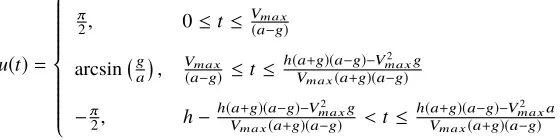
u(t)=

                   π

2, 0≤t ≤

Vm a x

(a−g)

arcsin ga

_, Vm a x

(a−g) ≤t ≤

h(a+g)(a−g)−V2 m a xg Vm a x(_a+g)(a−g)

−π

2, h−

h(a+g)(a−g)−V2 m a xg Vm a x(a+g)(a−g) <t≤

h(a+g)(a−g)−V2 m a xa Vm a x(a+g)(a−g)

(28)

For the values ofa,h,Vmaxandgused in this paper, the first switching time ists1 =41.667, the second switching time ists2=111.9048 and the final time istf =129.7619. This solution can be obtained in the same way as the analytic solution of the previous instance, by imposing continuity conditions across the switching points and solving for the

switching times.

For the second instance, two tests sets are presented: in the first set the order of the polynomials of both states and

controls are increased, while in the second set the order is constant but the number of elements is increased.

1. Problem Instance 2, test case 1

For test case 1 the time domain was discretised with 4 finite elements, and the order of the polynomials for both

states and controls was varied from 2 to 14.

Table 4 shows that the number of iterations to reach a feasibility is very marginally lower for Bernstein, while the

number of iterations to reach optimality is lower in the case of Bernstein basis expect for order 14. As in the previous

Table 4 Results for Problem Instance 2, Test case 1

Order Feas iter Opt iter Objective value

States Control La Bb La Bb La Bb

2 2 14 13 28 22 130.68 133.33

4 4 16 13 36 24 129.87 131.43

6 6 15 12 25 24 129.96 130.98

8 8 15 12 31 27 129.85 130.67

10 10 18 12 37 28 129.83 130.53

12 12 16 12 42 27 129.79 130.40

14 14 17 12 40 88 129.78 130.33

a

Lagrange basis.bBernstein basis.

but monotonically. The sparsity of the Jacobian is not shown because identical for both basis as in the previous instance

of the problem.

Figure 5 shows the time history ofufor both bases and different orders of the polynomials. While the control

laws obtained with the Legendre basis are veryoscillatory, especially when the path constraint is active, the variation

diminishing property of Bernstein polynomials is here fundamental, because the resulting polynomial solution will

oscillate less than the nodal solutions. In fact, while there are some small oscillations with Bernstein basis of order 2

and 6, which are due to a slightly oscillating nodal solution obtained by the NLP solver, the solution computed using

Bernstein basis presents no oscillations at order 12. Generally, oscillations in the control profile are to be expected when

path constraints are imposed on states and no higher order derivatives of the path constraint are provided to the NLP

solvers. This is fundamentally due to an indeterminacy of the control profile that satisfies the path constraint. It is

important to note that even if the value of the objective function converges faster for the Lagrange basis than for the

Bernstein basis, as the order increases, the control law in Bernstein basis is very close to the analytic solution while the

one in Lagrange basis is significantly different.

Figure 6 shows the time history of vy. The solutions of order 2 present discontinuities in the states. These

discontinuities are the sign that a polynomial solution of order 2 is inadequate to capture the dynamics. As the order of

the polynomials increases, the profile ofvyconverges to the analytical one (dashed line). With the Lagrange basis,

although the nodal values converge faster than Bernstein, some infeasible oscillations in the states are present, while

Bernstein basis remains feasible for all 0≤t≤tf.

2. Problem Instance 2, test case 2

For test case 2, similarly to test case 3 of Instance 1, problem 20 with path constraint 27 is solved with an increasing

number of finite elements but keeping their order constant.

(a) Lagrange basis: 4 elements of order 2 (b) Bernstein basis: 4 elements of order 2

(c) Lagrange basis: 4 elements of order 6 (d) Bernstein basis: 4 elements of order 6

(e) Lagrange basis: 4 elements of order 12 (f) Bernstein basis: 4 elements of order 12

(a) Lagrange basis: 4 elements of order 2 (b) Bernstein basis: 4 elements of order 2

(c) Lagrange basis: 4 elements of order 6 (d) Bernstein basis: 4 elements of order 6

(e) Lagrange basis: 4 elements of order 12 (f) Bernstein basis: 4 elements of order 12

Table 5 Results for Problem Instance 2, Test case 2

Number of Elements Feas iter Opt iter Objective value

La Bb La Bb La Bb

4 15 12 25 24 129.96 130.98

8 17 12 43 26 129.78 129.98

12 16 11 65 27 129.77 129.86

16 16 12 38 63 129.77 129.82

20 16 12 46 59 129.77 129.80

a

Lagrange basis.bBernstein basis.

this case, Bernstein basis is cheaper in most of the cases, up to a factor of 2.5, but becomes more expensive, by a factor

of almost 2, for high number of elements and converges slower to the exact value of the cost function. This will be

further investigated in the next subsection.

Figure 7 shows the time histories ofuas the number of elements is increased. For both bases, an increase in the

number of elements leads to the formation of high frequency oscillations in the nodal solutions when the path constraint

is active.The magnitude of these oscillations is however contained in the case of Bernstein and very high in the case of

Lagrange. Similarly to the previous case, even if the value of the objective function converges faster for the Lagrange

basis than for the Bernstein basis as the order is increased, the representation of the control law differs substantially:

with the Bernstein basis it’s very close to the analytic solution while with the Legendre case is very difficult to notice

any resemblance, even if one looks only at the nodal values.

The time history ofvyis shown in figure 8. Both bases converge quickly to the exact solution though Lagrange

presents some infeasible oscillations at low number of elements while Bernstein always remains within the feasible

region for all 0≤t ≤tf.

C. Effect of the NLP algorithm

All test cases were solved again with the SQP algorithm to check if a different NLP algorithm would give different

results in terms of convergence speed or value of the objective function, and to check and weather there are synergies

between the use of a particular choice of basis functions and an NLP algorithm.

Tables 6 to 10 show the number of iterations to reach optimality and the final value of the objective function for both

bases and NLP algorithms. In most cases the number of iterations remains fairly constant with respect to the size of the

problem. For the Lagrange basis, the number of iterations required by the SQP algorithm is approximately 50% more

than the Interior point algorithm, while for the Bernstein basis the SQP algorithm requires approximately 50% less

iterations than the Interior point algorithm. Moreover, with a single exception using the Interior point algorithm in Test

(a) Lagrange basis: 4 elements of order 6 (b) Bernstein basis: 4 elements of order 6

(c) Lagrange basis: 12 elements of order 6 (d) Bernstein basis: 12 elements of order 6

(e) Lagrange basis: 20 elements of order 6 (f) Bernstein basis: 20 elements of order 6

(a) Lagrange basis: 4 elements of order 6 (b) Bernstein basis: 4 elements of order 6

(c) Lagrange basis: 12 elements of order 6 (d) Bernstein basis: 12 elements of order 6

(e) Lagrange basis: 20 elements of order 6 (f) Bernstein basis: 20 elements of order 6

Table 6 Performance comparison of the NLP algorithms for Problem Instance 1, Test case 1

Order IP iterations IP Objective value SQP iterations SQP Objective value

States Control La Bb La Bb La Bb La Bb

2 2 40 27 109.19 109.62 51 8 109.19 109.62

4 4 37 29 109.25 109.35 54 16 109.25 109.35

6 6 36 28 109.08 109.30 50 21 109.08 109.30

8 8 35 32 109.15 109.23 71 10 109.15 109.23

10 10 35 21 109.12 109.22 41 9 109.19 109.22

12 12 42 26 109.12 109.20 32 11 109.12 109.20

14 14 37 28 109.12 109.18 37 12 109.12 109.18

Average 37.28 27.57 48.00 12.43

a

Lagrange basis.bBernstein basis.

Table 7 Performance comparison of the NLP algorithms for Problem Instance 1, Test case 2

Order IP iterations IP Objective value SQP iterations SQP Objective value

States Control La Bb La Bb La Bb La Bb

6 1 33 22 109.93 110.10 13 10 113.77 110.18

6 2 33 31 109.35 109.65 21 10 111.80 109.65

6 3 33 28 109.25 109.41 31 9 109.25 109.41

6 6 36 28 109.08 109.30 50 21 109.08 109.30

6 8 37 27 109.15 109.23 108 9 109.15 109.23

6 10 31 26 109.12 109.22 52 14 109.12 109.22

6 12 35 28 109.12 109.20 46 14 109.12 109.20

6 16 37 29 109.11 109.18 50 15 109.11 109.18

6 20 34 25 109.11 109.16 37 15 109.11 109.16

6 24 38 32 109.11 109.15 55 17 109.11 109.15

Average 37.40 27.60 46.30 13.40

a

Lagrange basis.bBernstein basis.

for Bernstein basis than for Lagrange basis, most of the times by a significant amount.

This shows an important interplay between the basis employed to represent the polynomials and the NLP algorithm.

This interplay is due to the different way the problem is represented in the numerical approximation, and the lower

number of iterations required by the Bernstein basis is very likely related to their superior numerical robustness as

explained in [19].

IV. Conclusions

This paper proposed the use of Bernstein polynomials as a basis for the DFET transcription of optimal control

Table 8 Performance comparison of the NLP algorithms for Problem Instance 1, Test case 3

Number of Elements IP iterations IP Objective value SQP iterations SQP Objective value

La Bb La Bb La Bb La Bb

4 36 28 109.08 109.30 50 21 109.08 109.30

8 33 28 109.10 109.17 54 15 109.10 109.17

12 37 35 109.10 109.14 62 15 109.10 109.14

16 46 34 109.11 109.12 54 18 109.11 109.12

20 40 45 109.11 109.11 64 23 109.11 109.11

Average 38.40 34.00 56.80 18.40

a

Lagrange basis.bBernstein basis.

Table 9 Performance comparison of the NLP algorithms for Problem Instance 2, Test case 1

Order IP iterations IP Objective value SQP iterations SQP Objective value

States Control La Bb La Bb La Bb La Bb

2 2 28 22 130.68 133.33 19 10 130.68 133.33

4 4 36 24 129.87 131.43 12 10 130.70 131.43

6 6 25 24 129.96 130.98 66 11 129.96 130.98

8 8 31 27 129.85 130.67 62 14 129.85 130.67

10 10 37 28 129.83 130.53 40 16 129.83 130.53

12 12 42 27 129.79 130.40 66 20 129.79 130.40

14 14 40 88 129.78 130.33 154 21 130.00 130.33

Average 34.14 34.29 59.86 14.57

a

Lagrange basis.bBernstein basis.

Table 10 Performance comparison of the NLP algorithms for Problem Instance 2, Test case 2

Number of Elements IP iterations IP Objective value SQP iterations SQP Objective value

La Bb La Bb La Bb La Bb

4 25 24 129.96 130.98 25 24 129.96 130.98

8 43 26 129.78 129.98 58 8 129.78 129.98

12 65 27 129.77 129.86 30 14 129.77 129.86

16 38 63 129.77 129.82 112 32 129.77 129.81

20 46 59 129.77 129.80 62 23 129.77 129.79

Average 46.17 39.83 62.00 19.50

a

which they inherit the convex hull and variation diminishing properties. A Theorem was proved, stating that, under some

general convexity conditions about the feasible region, this transcription scheme can guarantee that path constraints will

be satisfied everywhere in the time domain and not only at the quadrature nodes. These properties allow one to have

an everywhere feasible representation of the controls even in the case of a bang-bang or bang-zero-bang switching

structure. This fact was experimentally demonstrated with two different instances of a known optimal control problem.

It was also shown that the sparsity of the Jacobian of the constraint of the resulting NLP problem is comparable

to the one of DFET transcription schemes based on Lagrange polynomials on spectral basis. For this problem the

convergence of the NLP solver was faster than in the case of Lagrangian basis, however the convergence rate towards the

exact value of the cost function was slower.Furthermore, a slower convergence of the nodal values to the exact solution

was registered, as expected, given the slower convergence of Bernstein polynomials. This slower convergence rate is

expected to be present also in the case of continuous solutions, as demonstrated by other authors, but in the case of

jump discontinuities the convergence rate is comparable because of the unwanted oscillations of Lagrange bases, in

the neighbourhood of the discontinuity, for times different from the nodal values, that reduces the convergence rate to

O(₁)_{. On the the hand, when path constraints on the states were imposed, the use of Bernstein bases yielded solutions}

that displayed little or no oscillations of the controls along the path constraint even if no higher order derivatives were

provided to the NLP solver. In this case, the nodal solutions were also closer to the analytical solution than the nodal

solutions obtained with the Lagrange basis. A complete convergence theory of DFET on Bernstein basis is out of the

scope if this paper and is left for future work.

The smooth behaviour of Bernstein polynomials is retained when different orders are used for states and controls.

This property allows for flexible h/p adaptivity schemes which independently adapt the order of states and controls in

each element and avoid infeasible oscillations when the solution is interpolated on a new set of nodes.

Finally, an interesting interplay between the polynomial basis and the NLP algorithm was shown. In most cases, the

use of Bernstein basis required less iterations to converge to an optimal solution than the Lagrange basis. Depending

on the NLP algorithm and size of the problem, this difference was more or less significant, reaching a maximum of

one order of magnitude. This improved convergence rate of the NLP solver could be related to the superior numerical

robustness of Bernstein polynomials, previously demonstrated by other authors.

Acknowledgements

The research was partially funded by an ESA NPI grant (ref TEC-ECN-SoW-20140806) and Airbus Defence &

Space.

References

[2] Vasile, M., and Finzi, A. E., “Direct lunar descent optimisation by finite elements in time approach,”International Journal of

Mechanics and Control, Vol. 1, No. 1, 2000.

[3] Hodges, D. H., and Bless, R. R., “Weak Hamiltonian finite element method for optimal control problems,”Journal of Guidance,

Control, and Dynamics, Vol. 14, No. 1, 1991, pp. 148–156. doi:10.2514/3.20616, URLhttps://doi.org/10.2514/3.20616.

[4] Bottasso, C. L., and Ragazzi, A., “Finite Element and Runge-Kutta Methods for Boundary-Value and Optimal Control

Problems,”Journal of Guidance, Control, and Dynamics, Vol. 23, No. 4, 2000, pp. 749–751. doi:10.2514/2.4595, URL

https://doi.org/10.2514/2.4595_.

[5] Vasile, M., and Bernelli-Zazzera, F., “Optimizing low-thrust and gravity assist maneuvers to design interplanetary trajectories,”

Journal of the Astronautical Sciences, Vol. 51, No. No. 1, 2003.

[6] Vasile, M., and Bernelli-Zazzera, F., “Targeting a heliocentric orbit combining low-thrust propulsion and gravity assist

manoeuvres,”Operational Research in Space & Air, Vol. 79, 2003.

[7] Lorenzo A. Ricciardi, M. V., and Maddock, C., “Global solution of multi-objective optimal control problems with multi agent

collaborative search and direct finite elements transcription,”2016 IEEE Congress on Evolutionary Computation (CEC), IEEE,

2016. doi:10.1109/cec.2016.7743882, URLhttps://doi.org/10.1109/cec.2016.7743882.

[8] Vasile, M., and Ricciardi, L., “A direct memetic approach to the solution of Multi-Objective Optimal Control Problems,”

2016 IEEE Symposium Series on Computational Intelligence (SSCI), IEEE, 2016. doi:10.1109/ssci.2016.7850103, URL

https://doi.org/10.1109/ssci.2016.7850103_.

[9] Lorenzo Angelo Ricciardi, F. T., Massimiliano Vasile, and Maddock, C. A., “Multi-Objective Optimal Control of the Ascent

Trajectories of Launch Vehicles,”AIAA/AAS Astrodynamics Specialist Conference, American Institute of Aeronautics and

Astronautics, 2016. doi:10.2514/6.2016-5669, URLhttps://doi.org/10.2514/6.2016-5669.

[10] Lorenzo Ricciardi, C. M., and Vasile, M. L., “Multi-Objective Optimal Control of Re-entry and Abort Scenarios,”2018

Space Flight Mechanics Meeting, American Institute of Aeronautics and Astronautics, 2018. doi:10.2514/6.2018-0218, URL

https://doi.org/10.2514/6.2018-0218_.

[11] Vasile, M., “Finite Elements in Time: A Direct Transcription Method for Optimal Control Problems,”AIAA/AAS Astrodynamics

Specialist Conference, American Institute of Aeronautics and Astronautics, 2010. doi:10.2514/6.2010-8275, URLhttps:

//doi.org/10.2514/6.2010-8275_.

[12] Gzyl, H., and Palacios, J. L., “On the Approximation Properties of Bernstein Polynomials via Probabilistic Tools,”Bolet´ın de

la Asociaci´on Matem´atica Venezolana, Vol. X, No. 1, 2003.

[13] Rogalsky, T., “Bézier parameterization for optimal control by differential evolution,”International Conference on Genetic and

[14] Ghomanjani, F., Farahi, M., and Gachpazan, M., “Bézier control points method to solve constrained quadratic optimal

control of time varying linear systems,” Computational & Applied Mathematics, Vol. 31, No. 3, 2012, pp. 433–456.

doi:10.1590/s1807-03022012000300001, URLhttps://doi.org/10.1590/s1807-03022012000300001.

[15] Ghomanjani, F., and HadiFarahi, M., “Optimal Control of Switched Systems based on Bezier Control Points,”International

Journal of Intelligent Systems and Applications, Vol. 4, No. 7, 2012, pp. 16–22. doi:10.5815/ijisa.2012.07.02, URL

https://doi.org/10.5815/ijisa.2012.07.02_.

[16] Darehmiraki, M., Farahi, M. H., and Effati, S., “A Novel Method to Solve a Class of Distributed Optimal Control Problems Using

Bezier Curves,”Journal of Computational and Nonlinear Dynamics, Vol. 11, No. 6, 2016, p. 061008. doi:10.1115/1.4033755,

URLhttps://doi.org/10.1115/1.4033755.

[17] Mirkov, N., and Rasuo, B., “A Bernstein polynomial collocation method for the solution of elliptic boundary value problems,”

arXiv preprint arXiv:1211.3567, 2012.

[18] Bhatti, M. I., and Bracken, P., “Solutions of differential equations in a Bernstein polynomial basis,”Journal of Computational

and Applied Mathematics, Vol. 205, No. 1, 2007, pp. 272–280. doi:10.1016/j.cam.2006.05.002, URLhttps://doi.org/10.

1016/j.cam.2006.05.002_.

[19] Farouki, R., and Rajan, V., “On the numerical condition of polynomials in Bernstein form,”Computer Aided Geometric

Design, Vol. 4, No. 3, 1987, pp. 191–216. doi:10.1016/0167-8396(87)90012-4, URL

https://doi.org/10.1016/0167-8396(87)90012-4_.

[20] Betts, J. T.,Practical Methods for Optimal Control and Estimation Using Nonlinear Programming, Society for Industrial and

Applied Mathematics, 2010. doi:10.1137/1.9780898718577, URLhttps://doi.org/10.1137/1.9780898718577.

[21] Bottasso, C. L., “A new look at finite elements in time: a variational interpretation of Runge-Kutta methods,”Applied Numerical

Mathematics, Vol. 25, No. 4, 1997, pp. 355–368. doi:10.1016/s0168-9274(97)00072-x, URLhttps://doi.org/10.1016/

s0168-9274(97)00072-x_.

[22] Ait-Haddou, R., Nomura, T., and Biard, L., “A refinement of the variation diminishing property of Bézier curves,”Computer

Aided Geometric Design, Vol. 27, No. 2, 2010, pp. 202–211. doi:10.1016/j.cagd.2009.12.001, URLhttps://doi.org/10.

1016/j.cagd.2009.12.001_.

[23] Phillips, G. M.,Interpolation and approximation by polynomials, Springer, New York, 2003.

[24] Pallini, A., “Bernstein-type approximations of smooth functions,”Statistica; Vol 65, No 2 (2005); 169-191, 2007. doi:

10.6092/issn.1973-2201/84.

[25] Loock, W. V., Pipeleers, G., and Swevers, J., “Optimal motion planning for differentially flat systems with guaranteed

constraint satisfaction,” 2015 American Control Conference (ACC), IEEE, 2015. doi:10.1109/acc.2015.7171996, URL

[26] Cichella, V., Kaminer, I., Walton, C., and Hovakimyan, N., “Optimal Motion Planning for Differentially Flat Systems Using

Bernstein Approximation,”IEEE Control Systems Letters, Vol. 2, No. 1, 2018, pp. 181–186. doi:10.1109/lcsys.2017.2778313,

URLhttps://doi.org/10.1109/lcsys.2017.2778313.

[27] Açıkmeşe, B., and Blackmore, L., “Lossless convexification of a class of optimal control problems with non-convex

control constraints,”Automatica, Vol. 47, No. 2, 2011, pp. 341–347. doi:10.1016/j.automatica.2010.10.037, URLhttps:

//doi.org/10.1016/j.automatica.2010.10.037_.

[28] Blackmore, L., Açıkmeşe, B., and Carson, J. M., “Lossless convexification of control constraints for a class of nonlinear optimal

control problems,”Systems & Control Letters, Vol. 61, No. 8, 2012, pp. 863–870. doi:10.1016/j.sysconle.2012.04.010, URL

https://doi.org/10.1016/j.sysconle.2012.04.010_.

[29] Mao, Y., Dueri, D., Szmuk, M., and Açıkmeşe, B., “Successive Convexification of Non-Convex Optimal Control Problems

with State Constraints,”IFAC-PapersOnLine, Vol. 50, No. 1, 2017, pp. 4063–4069. doi:10.1016/j.ifacol.2017.08.789, URL