Abstract—It is a great challenge to differentiate Partial
Discharge (PD) induced by different types of insulation defects in high voltage cables. Some types of PD signals have very similar characteristics and are specifically difficult to be differentiate, even for the most experienced specialists. To overcome the challenge, a Convolutional Neural Network (CNN) based deep learning methodology for PD pattern recognition is presented in this paper. Firstly, PD testing for five types of artificial defects of Ethylene-Propylene-Rubber (EPR) cables is carried out in the High Voltage (HV) laboratory to generate signals containing PD data. Secondly, 3500 sets of PD transient pulses are extracted and then 33 kinds of PD features are established. The third stage applies a CNN to the data: typical CNN architecture and the key factors which affect the CNN based pattern recognition accuracy, are described. Factors discussed include the number of the network layers, convolutional kernel size, activation function, and pooling method. The paper presents the flowchart of the CNN based PD pattern recognition method and the evaluation with 3500 sets of PD samples. Finally, the CNN based pattern recognition results are shown and the proposed method is compared with two more traditional analysis methods, i.e. Support Vector Machine (SVM) and Back Propagation Neural Network (BPNN). The results show that the proposed CNN method has higher pattern recognition accuracy than SVM and BPNN, and that the novel method is especially effective for PD type recognition in cases of signals of high similarity, which is applicable for industrial applications.
Index Terms—Convolutional neural network, deep learning, high voltage cables, partial discharge, pattern recognition.
I. INTRODUCTION
ARTIAL Discharge (PD) monitoring plays an important role in evaluating the condition of cable insulation and in improving the reliability of power transmission and distribution system [1-5]. On-line or off-line PD based condition monitoring and fault diagnosis have been increasingly reported
Manuscript received October 31, 2018. This work was supported by Key Technological Project of China Southern Power Grid Co., Ltd. (GDKJXM20172769), and Natural Science Foundation of China (NSFC) 51807072.
Xiaosheng Peng, Fan Yang, Li Lee, Zhaohui Li and Ashfaque Ahmed are with State Key Laboratory of Advanced Electromagnetic Engineering and Technology, School of Electrical and Electronic Engineering, Huazhong University of Science and Technology, Wuhan, 430074, China.
Ganjun Wang and Yijiang Wu are with Zhongshan Power Supply Bureau of the Guangdong Power Grid Corporation, Guangdong, 528400, China.
Chengke Zhou and Donald M. Hepburn are with school of engineering and built environment, Glasgow Caledonian University, Glasgow, G4 0BA, UK.
Alistair Reid is with Cardiff School of Engineering, Cardiff University, Queen’s Buildings, The Parade, Cardiff, CF24 3AA, UK.
Martin D. Judd is with High Frequency Diagnostics and Engineering Ltd, Glasgow, G14 0BX, UK.
W. H. Siew is with Department of Electronic & Electrical Engineering, University of Strathclyde, Glasgow, G1 1XW, UK.
in industrial applications [6-7]. However, differentiating fault/defect type through PD pattern recognition is one of the most difficult challenges and this has restricted the large-scale industrial application of PD based condition monitoring. PD signals induced by insulation defects which show a high similarity in the PD pattern structure are especially difficult to distinguish [6-9].
To overcome the challenge of differentiating fault type, different pattern recognition methods have been used to detect PD patterns, e.g. Decision Tree (DT), Back Propagation Neural Network (BPNN), Support Vector Machine (SVM), and Rough Set (RS) Theory [10-12]. Among these methods SVM and BPNN have been widely used due to the excellent and stable pattern recognition performance [10-12]. In reference [10] Wavelet Transform (WT) and SVM are combined to recognize PD signals from different sources. In reference [11], Particle Swarm Optimization (PSO) is employed to optimize the parameters of SVM applied to distinguish PD signals from different sources in Gas Insulated Switchgear (GIS). In reference [12], two types of BPNN, with the input parameters of Phase Resolved Partial Discharge (PRPD) pattern and Time-Resolved Partial Discharge (TRPD) pattern, are combined to improve the pattern recognition accuracy of different types of PD signals from GIS.
However, it has been recognized that the traditional machine learning methods, such as SVM and BPNN, have met bottlenecks in their development, which restrict further improvement of the pattern recognition accuracy. In recent years, deep learning has been important in development of Artificial Intelligence (AI) and pattern recognition systems [13-15]. Deep learning methods use deep neural networks employing multiple nonlinear layers. These have the ability to capture high dimensional nonlinearity and complex correlation which cannot be learned by traditional shallow neural network structures [16]. Deep learning methods are capable of self-learning and feature abstracting from massive data, which brings new perspectives and opportunities for PD pattern recognition.
Typical deep learning methods comprise of Convolutional Neural Network (CNN), Stacked Denoising Auto-Encoders (SDAE), Recurrent Neural Network (RNN), Deep Belief Network (DBN), etc.: CNN is widely used [15]. CNN based deep learning algorithms have been successfully applied in many fields, such as speech recognition and image recognition, and are considered to be of increasing importance in the power industry [13-15]. In comparison to other deep learning methods, the complexity of CNN and the difficulty of training them are
A Convolutional Neural Network Based Deep Learning
Methodology for Recognition of Partial Discharge Patterns
from High Voltage Cables
Xiaosheng Peng, Fan Yang, Ganjun Wang, Yijiang Wu, Li Lee, Zhaohui Li, Ashfaque Ahmed Bhatti,
Chengke Zhou, Donald M. Hepburn, Alistair Reid, Martin D. Judd, W. H. Siew
greatly reduced through the parameters of sharing and local connection, which also reduce the risk of over-fitting [16]. According to [16], it is relatively easy to construct a network with deep architecture using CNN.
A CNN based deep learning methodology for PD pattern recognition of high voltage cables is presented in this paper and evaluated with 3500 sets of data. The data was generated using 5 types of PD fault under laboratory conditions. The proposed method is compared with two traditional machine learning methods, SVM and BPNN. The results show that CNN based PD pattern recognition is more effective than SVM and BPNN and especially effective at differentiating PD types where the patterns have high similarity. This method is applicable not only to PD pattern recognition in HV cables but also to analysis of signals from other HV apparatuses, such as GIS, transformers, generators, etc.
II. PD DATA GENERATION AND FEATURE EXTRACTION
A. EPR Cable and Artificial Defects
Five types of insulation defects found in EPR cables were simulated using a section of cable which has been in service. The artificial faults were stressed in a high voltage laboratory. The EPR cable comprises of an aluminum core, an inner semiconductor layer, an EPR layer, an outer semiconductor layer, a shielded copper strip, an aluminum armor layer and a polyvinyl chloride (PVC) sheath. A schematic of the EPR cable structure and a schematic of the defect structures are shown in
Fig. 1.
Defect type 1, simulating a void crossing from the PVC oversheath to the EPR insulation layer. The defect is obtained through the following procedure: a cylindrical cavity is generated by a precision 0.4 mm diameter Printed Circuit Board (PCB) drill, and the copper strip in contact with the outer semiconductor is fixed on the circular hole to seal the defect.
Defect type 2, simulating a protrusion on the outer conductor. Created by inserting a 0.4 mm diameter PCB drill into the cable. The drill remains in touch with the conductive parts.
Defect type 3, simulating a floating protrusion on the outer conductor. Created by inserting a PCB drill into the cable but ensuring that the conductive parts do not touch the drill.
Defect type 4, simulating a cable having external damage, has a breach in the outer semiconductor of the cable. To replicate this fault type, an area 7mm×7mm is cut from the PVC sheath, the semiconductor layer and the shielding layer.
Defect type 5 simulates PD from an end termination of a cable. It was generated by connecting a part of the outer copper sleeve
of the cable to the system earth.
Given the similarity of construction of defects type 2 and type 3, PD signals generated by these defects might be a challenge to separate.
B. Experimental Setup and PD Pulse Feature Extraction
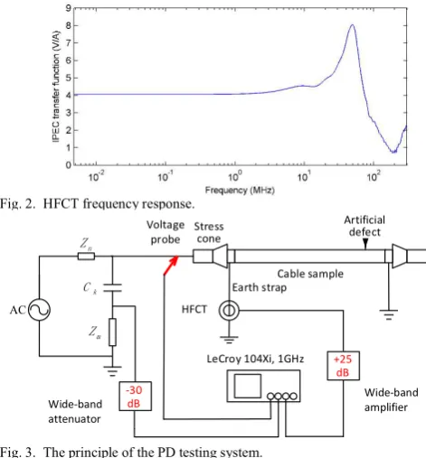
A commercial High Frequency Current Transformer (HFCT), having a bandwidth from 20 kHz to 20 MHz, as shown in Fig. 2, was applied for PD detection.
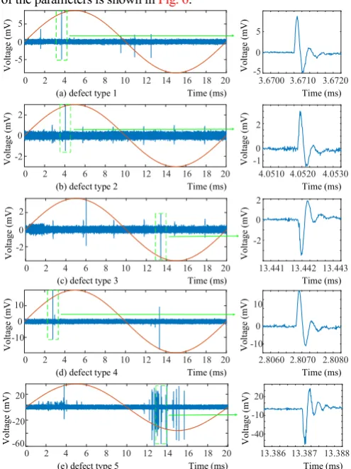
The principle of the PD testing system, which is based on the IEC60270 system, is shown in Fig. 3. EPR cable samples of length 1-2 meters, with the artificial defects described in section 1.1, were connected to the high voltage supply for PD testing. The HFCT was placed around the earth strap of the EPR cable to capture the PD signals. A wide-band amplifier was connected to the HFCT to adjust the signal from HFCT to the input limits of the data acquisition (DAQ) system, which is LeCroy 104 Xi oscilloscope. A voltage probe was connected to the high voltage source to get the 50 Hz phase signal for future PD pattern analysis. The DAQ rate of the oscilloscope was set to 100MS/s and the DAQ time length was set to 20ms, one power cycle of the 50Hz power supply.
The test voltage was increased from 0 to PD Inception Voltage (PDIV), in steps of 1kV, up to the maximum test voltage. For defect types 1, 4 and 5, the maximum value was 11kV, the rated voltage of the EPR cable. For defect types 2 and 3, the maximum voltage was 13 kV and 12 kV respectively. Raw data was logged for each test. The number of sets of raw PD data for each test voltage of the five types of defects is shown in Table 1.
From the raw data, PD transient pulses were extracted to generate PD data sets for five types of artificial defect. From the complete data 700 transient pulses were randomly selected from the data for each defect type for further analysis. This analysis relied upon feature extraction, as discussed in the Aluminium Core
Type 3 Type 2
Type 5
Type 4
Type 1 Inner semiconductor
EPR layer
Outer semiconductor
(Wound Cu tape) Sheath PVC over sheath
[image:2.595.305.541.344.598.2]Fig. 1. The cable structure and the artificial defects.
Fig. 2. HFCT frequency response.
LeCroy 104Xi, 1GHz
n Z
k C
m Z
HFCT
Artificial defect Voltage
probe Stress cone
Cable sample
+25 dB -30
dB Wide-band amplifier
Wide-band attenuator
Earth strap
AC
[image:2.595.58.252.439.530.2]following section.
TABLEI
PD TEST VOLTAGE AND NUMBER OF DATA SETS FOR EACH DEFECT TYPE Defect type 5 kV 6 kV 7 kV 8 kV 9 kV 10 kV 11 kV 12 kV 13 kV Sum Type 1 50 50 50 50 50 50 50 0 0 350 Type 2 0 50 50 50 54 50 54 53 52 409 Type 3 0 51 50 50 26 50 52 61 0 340 Type 4 0 0 50 50 51 52 51 0 0 254 Type 5 0 0 10 10 10 10 10 0 0 50
C. Feature Extraction
Based on the 3500 samples of PD transient pulses, feature extraction, in which important parameters of the signals are acquired, was carried out. The PD pulse signals are considered in terms of the following 17 parameters: pulse width [17], rise time [17], fall time [17], peak voltage, pulse polarity, mean voltage, root mean square (RMS) voltage, standard deviation of peak pulse voltage, skewness of peak pulse voltage, kurtosis of peak pulse voltage, voltage crest factor (peak magnitude over RMS), voltage form factor (RMS over average value), main frequency of transient pulse, phase angle, equivalent time length (T) [17], equivalent bandwidth (W) [17], discharge magnitude in pico Coulomb.
In addition to the 17 PD features described above, Wavelet Transform (WT) analysis was applied to the transient pulses [10]. The input signals were decomposed into five layers and 16 wavelet features were established for the wavelet transform. Finally, 33 types of PD features were constructed and were applied as the input parameters of the pattern recognition methods, BPNN, SVM, and CNN.
The principle of decomposition of PD to extract features of transient PD pulses is shown in Fig. 4.
In Fig. 4, the original transient PD pulses were decomposed into 5 layers based on a db5 mother wavelet. The wavelet features of the signals constructed according to the wavelet coefficients. Ai
represents the approximate composition of each layer. x represents the original signal. di represents the detail component of each
layer.
16 wavelet features are named as Ed1~ Ed5, Ea1~ Ea5, ED1~
ED5 and EA5 respectively.
Edi represents the detailed energy of layer i, the calculation
formula of which is shown in equation (1). 2( )
i i
Ed
d t dt (1)Eai represents the global energy of layer i, the calculation
formula of which is shown in equation (2). 2( )
i i
Ea
A t dt (2) EDirepresents the ratio of detail energy of layer i and the energyof the original signal, the calculation formula of which is shown in equation (3). 2 2 ( ) ( ) i i
d t dt ED
x t dt
(3) EA5 represents the ratio of global energy of the fifth layer and the energy of original signal x, the calculation formula of which is shown in equation (4).2 5
5 2
( ) ( ) A t dt EA
x t dt
(4)D. Initial Analysis
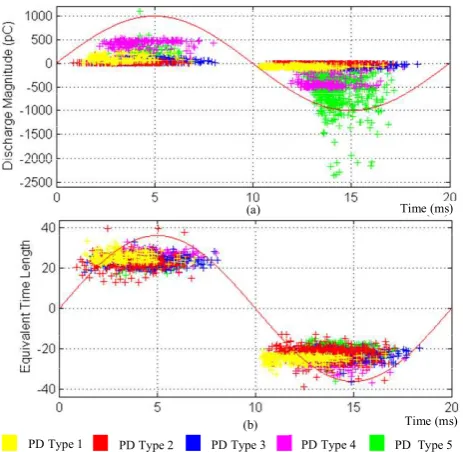
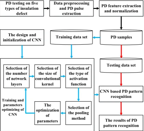
An initial comparison of the data from the five fault types was carried out. One set of PD raw data, with the time length of 20 ms, for each defect type, and one typical PD transient pulse for each defect type are shown in Fig. 5. Phase-Resolved PD Patterns were constructed using two different PD parameters, namely discharge magnitude, equivalent time length. The patterns generated for each of the parameters is shown in Fig.6.
0 2 4 6 8 10 12 14 16 18 20 -5 0 5 V ol ta ge ( m V ) Time (ms) (a) defect type 1
3.6700 3.6710 3.6720 -5 0 5 V ol ta ge ( m V ) Time (ms)
0 2 4 6 8 10 12 14 16 18 20 -2 0 2 V ol ta ge ( m V ) Time (ms) (b) defect type 2
4.0510 4.0520 4.0530 -1 0 2 V ol ta ge ( m V ) Time (ms)
0 2 4 6 8 10 12 14 16 18 20 -2 0 2 V ol ta ge ( m V ) Time (ms) (c) defect type 3
13.441 13.442 13.443 -2 0 2 V ol ta ge ( m V ) Time (ms)
0 2 4 6 8 10 12 14 16 18 20 -10 0 10 V ol ta ge ( m V ) Time (ms) (d) defect type 4
2.8060 2.8070 2.8080 -10 0 10 V ol ta ge ( m V ) Time (ms)
0 2 4 6 8 10 12 14 16 18 20 -60 20 V ol ta ge ( m V ) Time (ms) (e) defect type 5
13.386 13.387 13.388 -40 -10 20 V ol ta ge ( m V ) Time (ms) -20
Fig. 5. One set of PD raw data and one typical PD transient pulse for five types of cable defects.
From Fig.6, the following conclusions can be drawn: firstly, PD type 2, in red, and PD type 3, in blue, are very similar, as the two PRPD patterns of these faults overlap. This confirms the comment in section II.A. Secondly, PD type 4 and PD type 5 show differences to PD types 1, 2 and 3, e.g. in Fig. 5(a), the PRPD of discharge magnitude, data points for type 4 and 5 have a lower degree of overlap with PD type 1, 2 and 3.
From Fig. 5 and Fig. 6, the experimental data, 3500 sets of WT
Original signal (x)
Detail 1( )
Approax. 2( )
Detail 2( )
Approax. 3( )
Detail 3( )
Approax. 4( )
Detail 4( )
Approax. 5( )
Detail 5( )
1
d
Approax.
1( )A1 A2 A3 A4 A5
2
d d3 d4 d5
[image:3.595.304.552.309.640.2]
samples from 5 fault types were ideal data for pattern recognition method evaluation, as 3 types of PD signals had high similarity to each other and 2 types of PD signals had high similarity to each other, the similar data sets had low similarity to the others.
Additional analysis would be required to separate the fault types and the use of Convolutional Neural Networks was selected, as outlined in the following section.
PD Type 1 PD Type 2 PD Type 3 PD Type 4 PD Type 5
(b) Time (ms)
(a) Time (ms)Time (ms)
Fig. 6. PRPD of two parameters of five types of PD signals: (a) PD magnitude, (b) equivalent time length of PD.
III. CONVOLUTIONAL NEURAL NETWORK CNN was influenced by the structure of the biological vision system, which is with the ability to take specific features and figure out patterns in the visual images [15, 18]. In the 1960s, Hubel et al. discovered that visual information transmitted from the retina to the brain was processed by stimulating respective fields with multiple levels [18]. In 1980, Fukushima first proposed Neocognitron [18], which is a self-organizing multilayer neural network based on the theory of respective field. In 1998, LeCun et al. [19] proposed the first type of convolutional neural network, LeNet-5, by utilizing a gradient-based back propagation algorithm for supervised training. In 2012, Krizhevsky et al. won the image classification competition, ImageNet Large Scale Visual Recognition and Challenge, with AlexNet [20-21]. CNN is widely applied in image recognition and speech recognition because of the excellent feature learning ability.
A. Typical Architecture of CNN
The typical structure of CNN is shown in Fig.7. As shown in the lower layer labels, the CNN structure is comprised of one or more alternately connected convolutional layers, pooling layers and a fully connected layer for classification. In general, the input to a CNN is a 1 or 2 dimensional (1 or 2D) data matrix.
The convolutional layer is utilized directly to extract features from the 1D or 2D matrixes and map the extracted features to form new feature maps. The structure in which multiple convolutional layers are distributed with pooling layers allows the ability to
reduce the size of feature maps and gradually set up features with high degree of spatial and uniform structure. The fully connected layer is applied to estimate the PD pattern, based on the extracted features sequentially conveyed by multiple convolutional and pooling layers. In most cases CNN based pattern recognition systems are trained by gradient descent algorithm [18]. Originally, CNN is a mathematical model which shows raw input through data transformation and dimensionality reduction with multiple levels to a new feature representation field [18].
...
Features
Convolution Pooling Convolution Pooling connected Fully-Feature
maps
Feature maps
Feature maps
Feature maps
PD type
Fig. 7. The structure of CNN.
There are multiple key factors which affect the pattern recognition accuracy of CNN, including the number of network layers, the size of the convolutional kernel, the type of activation function and the pooling method, as discussed in the following section.
B. The Number of Network Layers
CNN have a special network structure in which the network nodes of the adjacent two layers are locally connected. In addition, CNN systems use shared parameters of connection weights in the same convolutional layers or pooling layers [18-20]. These characteristics greatly decrease the number of parameters, reduce the complexity of network training and the risk of over fitting
[18-20]. Therefore, CNN has great advantages in constructing deep architecture neural networks and provides superior feature learning capability [19].
As the number of network layers increases, the feature abstraction and capabilities of CNN increase gradually but the number of parameters required for training also increases and the need for sample data volume rises accordingly, which will raise the risk of over fitting for small sample data [21-22]. However, there is no theoretical framework on how to determine the number of network layers [18-20]. So for the success application of CNN based pattern recognition, different numbers of network layers should be evaluated with the training data. The network with the highest pattern recognition accuracy could be chosen as the ideal CNN architecture.
C. The Size of Convolutional Kernel
The CNN convolutional layer, the main block, has a series of convolutional kernels. During the forward propagation process, each convolutional kernel convolves with the input feature structure from the earlier layer to produce convolved feature maps. The convolved data is then subjected to a nonlinear activation function to get the output feature maps of the layer.
[image:4.595.49.281.169.395.2] [image:4.595.307.551.197.288.2]but at different locations in the input feature layout.
The size of the convolutional kernel affects the performance of feature detecting directly. Moreover, the material complexity of each convolutional operation in the CNN model is theoretically linear with the side length of the convolutional kernel. If the size of convolutional kernel is too small, then the CNN model is susceptible to information loss in the process of feature learning, which will negatively affect the pattern recognition performance. If the size of the convolutional kernel is too big, the computational cost rapidly increases [19].
a b c
e f g
i j k
m n
p q
Input
Kernel am+bn +ep+fq
bm+cn +fp+gq
em+fn +ip+jq
fm+gn +jp+kq Convolution
Output after convolution
Feature map
Fig. 8. Sample of convolution: a 2×2 kernel convolves with a 3×3 input feature map to produce a 2×2 feature map.
D. Nonlinear Activation Function
An activation function is used to introduce nonlinearities to the CNN, which plays an important role in determining the pattern recognition performance. Typical nonlinear activation functions contain hyperbolic tangent function (tanh), sigmoid, and rectified linear unit (relu) [21].
Google Brain proposed a new type of self-gated activation function, swish, which has an upper bound but no lower bound, accompanied with smooth and non-monotonic characteristics [21]. [21] pointed out that deep learning models with swish activation functions have better performance than the widely used relu activation function and that better results would be achieved by deep neural networks using swish if slightly smaller learning rate adopted compared with neural networks with relu [21].
As the saturation property of sigmoid functions have the challenges of gradient disappearing and high computational cost, it is difficult to effectively train the limits of deep neural networks with sigmoids [18-21]. The tanh function has similar saturation characteristic to sigmoids, giving rise to similar pattern recognition accuracy issues. In comparison to sigmoid and tanh, the linear and unsaturated characteristics of the relu function is favorable for making neural networks converge rapidly. However, some of the weights of nodes of the neural networks with relu may not be upgraded during training, i.e. a “dead zone” occurs. The absence of an upper bound and the smooth and non-monotonic characteristics are the advantages of the swish function over other existing activation functions.
E. Pooling Method
As the original input feature block has large number of features the computational cost may become excessive, i.e. if all the features from one convolutional layer are directly adopted. The pooling operation system is applied to collect semantically similar features in the pooling window within a feature structure into one feature. This helps to reduce the size of feature layout and achieve the goals of data dimensionality reduction [18-21].
There is some difference in the effectiveness of CNNs with
different pooling approaches on various data sets. Currently, max pooling and average pooling are the two main stream pooling methods [18-21].
For the convolved feature, the max pooling method selects the feature with the largest value within the pooling window to form the output feature. An example of max pooling method is shown in
Fig. 9. A 2×2 pooling window gets input from a convolved feature diagram and takes the feature with the greatest value in each window to generate a pooled feature. Max pooling discards non-maximal features and this may result in information loss.
7 3 2 7
5 6 7 8
3 2 1 0
1 2 3 4
7 8
3 4
Convolved feature Pooled feature
Pooling
Fig. 9. Sample of max pooling: convolved features are divided into disjoint four 2×2 regions, and take the maximum of each region to obtain the pooled features.
The average pooling method takes the average of the input features within the pooling window. Average pooling selects the average value of the features in the pooling window but this discrimination of data may also result in information loss.
The Rank based Average Pooling (RAP) method effectively handles the problem of the loss of useful information caused by average pooling and max pooling by weighted averaging the features in the pooling window [23]. RAP combines the advantages of max pooling and average pooling, therefore has a better performance as it retains the discriminatory features lost in average pooling and the non-maximal features absolutely discarded in max pooling [23].
IV.
CNN BASED PD PATTERN RECOGNITION PROCESSThe flowchart of the CNN based PD pattern recognition method for high voltage cables is shown in Fig.10.
PD samples PD testing on five
types of insulation defect
Training and parameters optimizing of
CNN
Selection of the number of network
layers
Selection of the size of convolutional
kernel
Selection of the type of
activation function
The optimization
of parameters The design and
initialization of CNN
Selection of the pooling method Data preprocessing
and PD pulse extraction
PD feature extraction and normalization
Training data set
Testing data set
CNN based PD pattern recognition
The results of PD pattern recognition
[image:5.595.369.492.205.289.2] [image:5.595.81.251.208.283.2] [image:5.595.307.542.517.731.2]The following steps explain the details of the schematic diagram of the presented method:
Step 1: Five types of artificial insulation defect in EPR cable were tested in the laboratory and the experimental data from PD testing was collected.
Step 2: The experimental data was pre-processed and PD pulses were extracted.
Step 3: 33 kinds of PD features were constructed and normalized and the features were used as the input to the CNN.
Step 4: The PD feature data set, containing 3500 sets of PD transient pulses, was established and divided into a training set and a testing set. The ratio of the number of training sets to testing sets was 8.5:1.5.
Step 5: The CNN architecture was designed and initialization of the CNN was performed. The gradient descent method was used on the training set to decrease the error rate between the predicted output and the actual output to train the CNN model. The ideal choice of the parameters, including the number of network layers, the convolutional kernel size, the activation function and the pooling methods, were determined.
Step 6: The performance of the CNN based PD pattern recognition method was evaluated on the testing set.
V. RESULTS AND EVALUATION
In this section, the PD pattern recognition results of CNN for high voltage cables were evaluated, in terms of number of network layers, the convolutional kernel size, the activation function and the pooling method. Furthermore, the proposed approach was compared with the traditional methods, i.e. BPNN and SVM.
The computer configuration was as follows: the operating system is Windows 7, the CPU is Intel i5-4200M and the memory size is 12 GB.
A. Results of PD Pattern Recognition of CNN with Different Number of Network Layers
The performance of CNN with different number of network layers was tested. The structure of each CNN had similar characteristics, i.e. the same number of convolutional and pooling layers and a single fully connected layer, for classification. In addition, the RAP pooling method, the swish activation function and convolutional kernel size of 1×4 were adopted. The first CNN had 3 layers (1 convolutional layer, 1 pooling layer and 1 fully connected layer), the second had 5 layers (2 convolutional, 2 pooling and 1 fully connected layer), up to the final CNN of 17 layers (8 convolutional, 8 pooling and 1 fully connected layer): results are shown in Fig.11.
As the number of network layers increases, the ability of CNN to fit the reference data will increase, but the risk of over-fitting also increases, especially when the sample data is small. As there are 3,500 samples in the data set, which is a relatively small number, the optimal number of network layers should be relatively small. As shown in Fig.11, among the 8 models generated, the 7-layer CNN has the highest overall PD pattern recognition accuracy and the highest pattern recognition accuracy for every type of defect.
A
cc
ur
ac
y
The layers of CNN
PD Type 1 PD Type 2 PD Type 3 PD Type 4 PD Type 5 Total
3 5 7 9 11 13 15 17
0.70 0.75 0.80 0.85 0.90 0.95 1.00
Fig. 11. Comparison of recognition error of CNN with different number of layers.
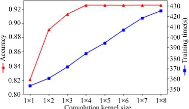
B. Results of PD Pattern Recognition of CNN with Different Convolutional Kernel Sizes
This section shows that CNN with 2-dimensional convolutional kernels, of size n×n, have difficulty with conducting network training and have non-ideal performance owing to a significant increase in the number of network parameters, compared to CNN with 1-dimensional convolutional kernels of size 1×n. Hence, the PD pattern recognition results of CNNs with convolutional kernel sizes of 1×1 to 1×8 are presented. Based on the previous section, the number of network layers was set to 7 and the other parameter settings are the same as those shown in section V.A. Test results are shown in Fig.12.
Convolution kernel size 0.80
0.82 0.84 0.86 0.88 0.90 0.92
A
cc
ur
ac
y
350 360 370 380 390 400 410 420 430
T
ra
in
in
g
tim
e(
s)
1×1 1×2 1×3 1×4 1×5 1×6 1×7 1×8
Fig. 12. Comparison of recognition error of CNN with different convolution kernel sizes.
[image:6.595.323.502.83.217.2] [image:6.595.339.532.399.510.2]performance of CNN in section III.C.
C. Results of PD Pattern Recognition of CNN with Different Activation Functions
The type of activation function applied strongly affects the effectiveness of CNN pattern recognition [21]. In this paper, the pattern recognition performance of CNNs with four activation functions, namely tanh, sigmoid, relu and swish, was compared,
using a convolutional kernel size of 1×4 but retaining the other parameters as outlined in section V.B. The results are shown in
Fig.13.
From Fig. 13, the swish function has a higher pattern recognition accuracy than CNNs with the other three activation functions.
swish relu tanh sigmoid
A cc ur ac y 0.60 0.70 0.80 0.90 1.00
1 2 3 4 5
PD type
Fig. 13. Comparison of recognition accuracy of CNN using 4 activation functions.
D. Results of PD Pattern Recognition of CNN Using Different Pooling Methods
The PD pattern recognition performance of CNNs with three pooling methods, i.e. average pooling, max pooling and RAP, are compared. The activation function adopted is swish, other parameters are the same as those in section V.C. The results are shown in Fig.14.
From Fig. 14, CNN with RAP has the highest PD pattern recognition accuracy for every type of PD fault type. As discussed, RAP has the ability to merge the advantages of average pooling and max pooling, resulting in CNN with RAP having the best PD pattern recognition performance. The overall pattern recognition accuracy of CNN with RAP is 92.57%, which is 0.57% and 0.76% better than CNNs adopting max pooling and average pooling, respectively.
PD type Average pooling Max pooling 0.60 0.70 0.80 0.90 1.00 A cc ur ac y
1 2 3 4 5
RAP
Fig. 14. Comparison of recognition error of CNN using 3 pooling methods.
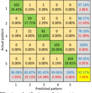
E. Pattern Recognition Results and Visualization of CNN
Based on the foregoing analysis, the final adopted architecture of CNN contains 3 convolutional layers, 3 pooling layers and 1 fully connected layer for classification. The other
parameter configurations of CNN in this work are RAP pooling, swish activation function and convolutional kernel size of 1×4. The confusion matrix for PD pattern recognition of CNN is shown in Fig.15.
As can be seen in Fig. 15, high error rates exist for defect types with high similarity, namely PD type 2 and type 3. The degree of confusion among the PD pattern recognition results of defect types 2 and 3 are: 21 of the 105 samples of defect type 3 are misidentified as type 2; 12 of the 105 samples of defect type 2 were misidentified as type 3. The result verifies the analysis of PRPD in section 1.3 and is the main reason for the need to improve overall PD pattern recognition accuracy.
0
0.00% 0.00%0 0.00%0 0
0.00% 0.00%0 0.00%0
98.08%
1.92% 80.87%19.13% 85.42%14.58%
2
0.38% 4.00%21 15.62%82 105 20.00% 1 0.19% 99.06% 0.94% 0 0.00% 0
0.00% 17.71%93 2.29%12 0.00%0 102
19.43% 0.19%1 0.38%2 0.00%0
0 0.00% 104 19.81% 100% 0.00% 0 0.00% 0 0.00% 0 0.00% 100% 0.00% 99.05% 0.95% 92.57% 7.43% 78.10% 21.90% 88.57% 11.43% 97.14% 2.86%
1 2 3 4 5 5 4 3 2 1 Predicted pattern Ac tu al p at te rn
Fig. 15. PD pattern classification confusion matrix.
In order to illustrate the feature abstracting and expressing capabilities of CNN, the t-SNE algorithm was applied to map the original PD features and the output of each convolutional layer of CNN to a two-dimensional plane for visualization [24]. The results are shown in Fig. 16. The t-SNE algorithm is a non-linear dimensionality reduction technique: further information on t-SNE can be found in [24].
In Fig.16 it can be observed that data points for each defect type are grouped together in the original feature space. As expected the degree of overlap for points corresponding to defect types 2 and 3 are particularly large.
PD Type 1
-60 -40 -20 0 20 40 60 80 -60 -40 -20 0 20 40 60
-80 -60 -40 -20 0 20 40 60 80 -60 -40 -20 0 20 40 60 D im en si on 2 D im en si on 2
(c) 2nd Convolution layer -60 -40 -20 0 20 -60 -40 -20 0 20 40
40 60 80
D im en si on 2 Dimension 1 60 40 20 0 20 40 60 -60 -40 -20 0 20 40 60 D im en si on 2
(a) the original feature space (b) 1st Convolution layerDimension 1
PD Type 2 PD Type 3 PD Type 4 PD Type 5 Dimension 1
(d) 3rd Convolution layerDimension 1
Fig. 16. 2D visualization of the original feature space and the convolutional layer output.
[image:7.595.333.492.227.388.2] [image:7.595.63.250.248.365.2] [image:7.595.305.550.525.707.2] [image:7.595.67.250.571.690.2]observed that as the number of convolutional layers increases, the samples matching to the five defect types become systematically more separated. After being processed by the first convolutional layer, the clusters of five fault types have a greater degree of separation than those in the original feature space: the discrimination of types 1, 4 and 5 is relatively large.
After being processed by the second convolutional layer, the relative separation of the five types of defect is greater than those in the previous convolutional layer. After being handled by the third convolutional layer, the samples point clusters are more concentrated and differentiable from each other. The contribution of each convolutional layer of CNN to distinguish the complementary samples of the five types of defect is visually indicated in Fig.16, representing the principle of the layer-wise optimization of the deep neural network.
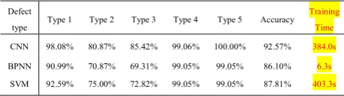
F. Comparison with the Traditional Pattern Recognition Methods
To express the advantages of PD pattern recognition based on the CNN method, PD pattern recognition by BPNN and SVM was also studied. Comparative results are shown in Table 2.
TABLEII
COMPARISON OF PD PATTERN RECOGNITION ACCURACY RATES OF DIFFERENT ANALYSIS METHODS
Defect
type Type 1 Type 2 Type 3 Type 4 Type 5 Accuracy
Training Time
CNN 98.08% 80.87% 85.42% 99.06% 100.00% 92.57% 384.0s
BPNN 90.99% 70.87% 69.31% 99.05% 99.05% 86.10% 6.3s
SVM 92.59% 75.00% 72.82% 99.05% 99.05% 87.81% 403.3s From Table 2, overall PD pattern recognition accuracy rate of CNN is 92.57%, which was the highest among the three methods. The overall accuracy of SVM is 87.81% and that of BPNN was 86.10%, BPNN was lowest among of the approaches. Compared to BPNN and SVM, overall pattern recognition accuracy of CNN was increased by 6.47% and 4.76%, respectively. Furthermore, the pattern recognition accuracy of CNN for every type of defect was the highest among all methods. The degree of distinction of defect types 1, 4, and 5 is relatively high, making it easier to differentiate the three defect types. PD pattern recognition accuracy rates of CNN for fault types 1, 4 and 5 are 98.08%, 99.06%, and 100.00%, respectively. As discussed, defect types 2 and 3 have high similarity. CNN has a PD pattern recognition accuracy for defect type 2 of 80.87%, which was 10.00% and 5.87% better than BPNN and SVM. The accuracy of CNN for defect type 3 is 85.42%, which was 16.11% and 12.60%, better than BPNN and SVM respectively.
One disadvantage of CNN is that the method takes more training time than BPNN. The training time of CNN is 384.0 seconds and the training time of BPNN is 6.3 seconds. The training time of SVM is 403.3 seconds, which is close with CNN. The testing time for different methods, CNN, BPNN and SVM, is less than 1 second.
VI. CONCLUSIONS AND DISCUSSIONS
A convolutional neural network based deep learning method
for PD pattern recognition of different types of insulation defects in HV cables was explained. The proposed technique was compared with traditional SVM and BPNN methods. The conclusions drawn were as follows:
The CNN based PD pattern recognition method proposed here is proven to be effective, evaluated with 3500 sets of PD samples obtained from experiment. The overall pattern recognition accuracy of PD signals from five types of defect is 92.57%, an increase of 6.47% and 4.76% compared with BPNN and SVM.
The proposed CNN based PD pattern recognition is also effective for defect types with high similarity, e.g. type 2 and type 3 PD. The PD pattern recognition accuracy of CNN for defect type 2 was 10.00% and 5.87% better than BPNN and SVM respectively. The accuracy of CNN for defect type 3 was 16.11% and 12.60% better than BPNN and SVM.
As outlined in the paper, the structure of the CNN, i.e. the number of network layers, the convolutional kernel size, the activation function and the pooling method applied, affects the accuracy of the CNN based PD pattern recognition method.
As the number of network layers increases, the ability of CNN to correct the reference data increases. Based on the dataset used in this work, a 7-layer CNN has the highest overall PD pattern recognition accuracy and the highest accuracy for each type of defect.
The size of the convolutional kernel has significant impact on the CNN based PD pattern recognition accuracy. For this dataset a convolutional kernel size of 1×4 is shown to be most accurate and to have moderate computational cost. Based on the dataset, the overall pattern recognition accuracy for the five types of PD signals based on CNN with swish was better by 3.43%, 2.56% and 0.95%, compared with CNNs with tanh, sigmoid, and relu, respectively.
The overall accuracy rate for PD pattern recognition based on CNN with RAP was better by 0.57% and 0.76%, compared with CNNs with max pooling and average pooling systems respectively.
All studies in the paper were based on laboratory simulated artificial defects. The major reason is, for most on-line PD monitoring systems or on-site PD testing it is difficult to correlate PD signals with corresponding cable defect types if cable maintenance is not carried out after PD signals are detected. Whether the pattern recognition methods based on artificial defects could be applied to actual defects or not depends on whether the artificial defects are the same as the real defects.
[image:8.595.44.290.354.423.2]REFERENCES
[1] J. Li, X. Han, Z. Liu,X. Yao. “A novel GIS partial discharge detection sensor with integrated optical and UHF methods,” IEEE Trans. on Power Del., vol. 33, no. 4, pp. 2047-2049, Aug. 2018.
[2] A. Krivda, “Automated recognition of partial discharges,” IEEE Trans. Dielectr. Electr. Insul.,vol. 2, no. 5, pp. 796-821, Oct. 1995.
[3] R. Wu, C. Chang. “The use of partial discharges as an online monitoring system for underground cable joints,” IEEE Trans. on Power Del., vol. 26, no. 3, pp. 1585-1591, Jul. 2011.
[4] Z. Hou, H. Li, Z. Sun, B. Liu, S. Ji, C. Zhu. “A novel sinusoidal damped oscillating voltage generator for the detection of partial discharge in MV distribution power cables,” IEEE Trans. on Power Del., vol. 31, no. 1, pp. 410-411, Feb. 2016.
[5] T. Shao, F. Kong, H. Li, Y. Ma, Q. Xie, C. Zhang. “Correlation between Surface Charge and DC Surface Flashover of Plasma Treated Epoxy Resin,” IEEE Trans. Dielectr. Electr. Insul.,vol. 25, no. 4, pp. 1267-1274, Aug. 2018.
[6] A. Hirata, S. Nakata, Z. I. Kawasaki. “Toward automatic classification of partial discharge sources with neural networks,”
IEEE Trans. on Power Del., vol. 21, no. 1, pp. 526-527, Jan. 2006. [7] C. S. Chang, J. Jin, C. Chang, T. Hoshino, M. Hanai, N. Kobayashi.
“Separation of corona using wavelet packet transform and neural network for detection of partial discharge in gas-insulated substations,” IEEE Trans. on Power Del., vol. 20, no. 2, pp. 1363-1369, Apr. 2005.
[8] D. Antony, G. S. Punekar. “Noniterative method for combined acoustic-electrical partial discharge source localization,” IEEE Trans. on Power Del., vol. 33, no. 4, pp. 1679-1688, Aug. 2018. [9] L. Zhu, F. Hou, S. Ji, H. Rehman, X. Wu. “Primary differential pulse
method for partial-discharge detection of oil-immersed inverted current transformers,” IEEE Trans. on Power Del., vol. 33, no. 3, pp. 1492-1494, Jun. 2018.
[10] L. Hao, P. L. Lewin. “Partial discharge source discrimination using a support vector machine,” IEEE Trans. Dielectr. Electr. Insul.,vol. 17, no. 1, pp. 189-197, Feb. 2010.
[11] J. Tang, F. Liu, X. Zhang, Q. Fan. “Partial discharge recognition based on SF6 decomposition products and support vector machine,”
IET Sci. Meas. Technol., vol. 6, no. 4, pp. 198-204, Jul. 2012. [12] L. Li, J. Tang, Y. Liu. “Partial discharge recognition in gas insulated
switchgear based on multi-information fusion,” IEEE Trans. Dielectr. Electr. Insul.,vol. 22, no. 2, pp. 1080-1087, Apr. 2012.
[13] S. Hui, J. Dai, G. Sheng, X. Jiang. “GIS partial discharge pattern recognition via deep convolutional neural network under complex data source,” IEEE Trans. Dielectr. Electr. Insul., vol. 25, no. 2, pp. 678-685, Apr. 2018.
[14] G. Li, X. Wang, X. Li, A. Yang, M. Rong. “Partial discharge recognition with a multi-resolution convolutional neural network,”
Sensors, vol. 18, no. 10, pp. 3512, Oct. 2018.
[15] F. Liu, C. Shen, G. Lin, I. Reid. “Learning Depth from Single Monocular Images Using Deep Convolutional Neural Fields,” IEEE Trans. Pattern Anal. Mach. Intell., vol. 38, no. 10, pp. 2024-2039, Oct. 2016.
[16] S. H. Bae, K. J. Yoon. “Confidence-Based Data Association and Discriminative Deep Appearance Learning for Robust Online Multi-Object Tracking,” IEEE Trans. Pattern Anal. Mach. Intell.,vol. 40, no. 3, pp. 595-610, Mar. 2018.
[17] X. Peng, J. Wen, Z. Li, G. Yang, C. Zhou, A. Reid, D. M. Hepburn, M. D. Judd, W. H. Siew. “Rough set theory applied to pattern recognition of Partial Discharge in noise affected cable data,” IEEE Trans. Dielectr. Electr. Insul., vol. 24, no. 1, pp. 147-156, Feb. 2017. [18] Y. P. LEE. “Multidimensional hebbian learning with temporal coding
in neocognitron visual recognition,” IEEE Trans. Syst., Man, Cybern., vol. 47, no. 12, pp. 3386-3396, Dec. 2017.
[19] C. Dong, C. C. Loy, K. He, X. Tang. “Image super-resolution using deep convolutional networks,” IEEE Trans. Pattern Anal. Mach. Intell., vol. 38, no. 2, pp. 295-307, Feb. 2016.
[20] J. Zhang, H. P. H. Shum, J. Han, L. Shao. “Action recognition from arbitrary views using transferable dictionary learning,” IEEE Trans. Image Process., vol. 27, no. 10, pp. 4709-4723, Oct. 2018.
[21]D. Liu, Z. Wang, Y. Fan, X. Liu, Z. Wang, S. Chang, X. Wang, T. S. Huang. “Learning temporal dynamics for video super-resolution: a deep learning approach,” IEEE Trans. Image Process., vol. 27, no. 7, pp. 3432-3435, Jul. 2018.
[22]S. S. S. Kruthiventi, K. Ayush, R. V. Babu. “DeepFix: A Fully Convolutional Neural Network for Predicting Human Eye Fixations,”
IEEE Trans. Image Process., vol. 26, no. 9, pp. 4446-4456, Sept. 2017.
[23]S. Wang, Y. Jiang, X. Hou, H. Cheng, S. Du. “Cerebral Micro-Bleed Detection Based on the Convolution Neural Network With Rank Based Average Pooling,” IEEE Access, vol. 5, pp. 16576–16583, Aug. 2017.
[24]J. Cheng, H. Liu, F. Wang, H. Li, C. Zhu. “Silhouette Analysis for Human Action Recognition Based on Supervised Temporal t-SNE and Incremental Learning,” IEEE Trans. Image Process., vol. 24, no. 10, pp. 3203-3217, Oct. 2015.
Xiaosheng Peng (M’11) received the B.Sc. and M.Sc. degrees from Huazhong University of Science and Technology, China in 2006 and 2009, respectively, and the Ph.D. in electrical engineering at Glasgow Caledonian University in 2012 funded by EPSRC. He has worked as a postdoctoral research fellow in Glasgow Caledonian University funded by EDF Energy. He is currently an associated professor in School of Electrical and Electronic Engineering of Huazhong University of Science and Technology. His research interests are partial discharge signal processing and condition monitoring of power plant. He is a member of IET.
Chengke Zhou (M’06) received the B.Sc. and M.Sc. degrees in electrical engineering from Huazhong University of Science and Technology, China in 1983 and 1986, respectively, and the Ph.D. degree from the University of Manchester U.K., in 1994. Since then, he worked in Glasgow Caledonian University, U.K., as a Lecturer, Senior Lecturer and in Heriot-Watt University as a Reader until 2007 when he returned to Glasgow Caledonian University as a Professor. He has published over 100 papers in the area of PD based condition monitoring of MV/HV plant and power system analysis. He is member of IET.
Donald M. Hepburn received his B.A. (Hons) from the Open University in 1987 and the Ph.D. degree from Glasgow Caledonian University (GCU) in 1994. He has many years of industrial research experience and has been involved in research into high voltage insulation systems at GCU for over 20 years. His research interests cover monitoring of chemical changes to insulation materials, application of electrical, acoustic and RF monitoring equipment to HV components and application of advanced digital signal processing to information from the monitoring techniques. He is a Senior Lecturer at GCU and is involved in industrial and academic research projects.
Martin D. Judd (M'02-SM'04) is Technical Director of High Frequency Diagnostics based in Glasgow, Scotland. He was born in Salford, England in 1963 and graduated from the University of Hull in 1985 with a 1st
Class (Hons) degree in Electronic Engineering, after which he gained 8 years of industrial experience with both Marconi Electronic Devices and EEV Ltd. Martin received his PhD degree from the University of Strathclyde in 1996 for research into the excitation of UHF signals by partial discharges in gas insulated switchgear. He has worked extensively on UHF partial discharge location techniques for power transformers and was latterly Professor of High Voltage Technologies at the University of Strathclyde, where he managed the High Voltage Research Laboratory. In 2014, he founded High Frequency Diagnostics, a specialist consultancy business that works in partnership with companies developing new electromagnetic wave sensor technologies and applications.