A Drift-Diffusion Model of Interval Timing in the Peak Procedure

(1)

City, University of London Institutional Repository

Citation

:

Luzardo, A., Rivest, F., Alonso, E. and Ludvig, E. (2017). A Drift-Diffusion Model

of Interval Timing in the Peak Procedure. Journal of Mathematical Psychology, 77, pp.

111-123. doi: 10.1016/j.jmp.2016.10.002

This is the accepted version of the paper.

This version of the publication may differ from the final published

version.

Permanent repository link:

http://openaccess.city.ac.uk/15472/

Link to published version

:

http://dx.doi.org/10.1016/j.jmp.2016.10.002

Copyright and reuse:

City Research Online aims to make research

outputs of City, University of London available to a wider audience.

Copyright and Moral Rights remain with the author(s) and/or copyright

holders. URLs from City Research Online may be freely distributed and

linked to.

City Research Online:

http://openaccess.city.ac.uk/

publications@city.ac.uk

(2)

A Drift-Diffusion Model of Interval Timing in the Peak

Procedure

Andr´e Luzardoa,∗, Fran¸cois Rivestb, Eduardo Alonsoa, Elliot A. Ludvigc

a_{Department of Computer Science, City University London, London, United Kingdom} b_{Mathematics and Computer Science, Center for Neuroscience Studies, Royal Military}

College of Canada - Queen’s University, Kingston, Ontario, Canada c_{Department of Psychology, University of Warwick, Coventry, United Kingdom}

Abstract

Drift-diffusion models (DDMs) are a popular framework for explaining response times in decision-making tasks. Recently, the DDM architecture has been used to model interval timing. The Time-adaptive DDM (TDDM) is a physiolog-ically plausible mechanism that adapts in real-time to different time intervals while preserving timescale invariance. One key open question is how the TDDM could deal with situations where reward is omitted, as in the peak procedure—a benchmark in the timing literature. When reward is omitted, there is a consis-tent pattern of correlations between the times at which animals start and stop responding. Here we develop a formulation of the TDDM’s stationary proper-ties that allows for the derivation of such correlations analytically. Using this simplified formulation we show that a TDDM with two thresholds–one to mark the start of responding and another the stop–can reproduce the same pattern of correlations observed in the data, as long as the start threshold is allowed to be noisy. We confirm this by running simulations with the standard TDDM formulation and show that the simplified formulation approximates well the full model under steady-state conditions. Moreover, we show that this simpli-fied version of the TDDM is formally equivalent to Scalar Expectancy Theory (SET) under stationary behaviours, the most prominent theory of interval tim-ing. This equivalence establishes the TDDM as a more complete drift-diffusion based theory with SET as a special case under steady-state conditions.

Keywords: interval timing, peak procedure, computational models, drift-diffusion model, scalar expectancy theory

1. Introduction

Learning the time between important events is a fundamental feature of cognition. Humans and other animals can readily learn the timing of upcoming

∗_{Corresponding author}

(3)

rewards and adapt their behavior accordingly [1, 2]. A range of psychological and computational theories have been proposed for interval timing [3, 4, 5, 6,

5

7, 8, 9] which succeed at capturing the broad outlines of timing behaviour, but they often flounder when dealing with the statistics of the micro-structure of real-time responding.

Particularly vexing for timing models are the behavioural patterns when predictably-timed rewards are occasionally omitted, as in the peak procedure

10

[10]. This peak procedure is likely the most popular interval timing task. Al-though major timing models such as Scalar Expectancy Theory (SET)[3], Be-havioral Theory of Timing (BeT)[4], Learning to Time (LeT)[11, 8] and Multiple Time Scales (MTS)[5] can reproduce the global averaged behaviour in this task, very few models have been able to account for the pattern of behaviour observed

15

in individual trials. The notable exception is SET, which provides good quan-titative fits to animal data [12] and remains the theory of choice for explaining static timing phenomena.

Recently, a series of studies have adapted the classic drift-diffusion model (DDM) used to explain the dynamics of real-time decision-making in behaviour

20

and the brain [13, 14, 15] to interval timing [9, 16, 17, 18]. The Time-adaptive DDM (TDDM) explains timing as the result of a noisy drift-diffusion process with an adaptive drift rate, which is adjusted based on the time interval ob-served. The TDDM has a plausible neural implementation, in that the for-malism is also a mathematical approximation of the net effect of excitation

25

and inhibition in the activity of a pool of neurons [18]. The model builds on earlier theories, such as SET, by adopting a different, more complete mathemat-ical formulation that allows modeling the trial-by-trial dynamics of timing (i.e., the learning), while still explaining core properties of interval timing (such as timescale invariance). The general modular architecture (accumulator, memory

30

storage and decision rules) is preserved, however, raising interesting questions as to the exact formal relationship between the TDDM and SET.

The TDDM has been successfully applied to some key features of interval timing. Most notably, it can account for the scalar property, a ubiquitous feature of timing data where the distribution of response times scales with the

35

interval being timed. The model has also been shown to learn quickly and to reproduce the behaviour observed in fixed-interval schedules [17], the bisection procedure [19], and tasks where time intervals are changing either randomly [18] or cyclically [16], but has been only cursorily applied to the aggregate data in the peak procedure thus far [9].

40

One of the main advantages of a mathematical model is the capacity to de-rive precise quantitative predictions from as few assumptions as possible. In this respect, the TDDM is particularly well placed among other timing models. As previously demonstrated [9], Weber’s law, which in the context of interval timing manifests itself as a constant coefficient of variation (CV), follows from

45

(4)

is so large as to overcome the noise in the pacemaker. This solves the problem

50

but at the cost of adding an extra assumption and doing away with the Poisson pacemaker.

In this paper, we show that the TDDM can account for both the global averaged response curve in the peak procedure—and reproduce the statistics of behaviour in individual trials. We demonstrate this first analytically, through

55

a new simplified formulation of TDDM’s stationary properties, which we then show is equivalent to a constrained version of SET. The analytical results from the simplified model are then validated through simulations with the complete TDDM formulation.

These results extend the range of phenomena for which the TDDM can

60

account and suggest that the Poisson pacemaker postulated by SET—but not actually used—may be substituted by the result of an opponent Poisson process [9]. Furthermore, and in light of previous successes, these results suggest there might be a single comprehensive drift-diffusion-based theory of decision making and timing, which could cover both the steady-state properties as well as the

65

learning dynamics.

The paper next reviews the studies that have examined the patterns of cor-relations in single-trial analyses of the peak procedure. We then revisit the TDDM and develop a simplified stochastic model approximating TDDM’s sta-tionary properties. Given that formulation, the simplest possible extension of

70

TDDM to support start and stop behaviours is analytically derived. This sim-plified formulation is shown to be equivalent to a constrained version of SET with two thresholds [12], and shown to be a good approximation of the full TDDM through simulations. Finally, some predictions are made with the full TDDM about possible sequential effects in the peak procedure.

75

1.1. Peak Procedure

In the peak procedure subjects are first trained on a fixed-interval (FI) sched-ule where the first response after an interval has elapsed since the appearance of a stimulus produces a reward (see diagram on the left in Fig. 1). When behavior on FI trials has stabilized, peak trials are then introduced. These peak trials

80

are interspersed randomly between the normal FI trials, last 3 or 4 times longer, and are not rewarded. When peak trials are first introduced during training, animals start responding as usual before the FI time and then continue respond-ing throughout the whole (long) interval. With sufficient experience with the peak trials, a different pattern emerges where responding eventually ceases or

85

lowers in frequency soon after the expected reward time [20]. This pattern of starts and stops that appears after sufficient training is the focus of our analysis here.

The panel on the right in Fig. 1 shows an example of how, when response rate is averaged over these peak trials even for a single individual, there is an

90

(5)

[image:5.612.154.459.133.316.2]

Figure 1: Peak procedure. Left: Schematic of fixed-interval (FI) and peak trials. Right: Response rate averaged over peak trials for one rat subject (data from [21]). Reward was ordinarily available after 20 seconds.

again after the usual interval has elapsed and no reward has arrived [22, 12, 23].

95

This three-state system (low-high-low) can be characterized by its two transition points: the start (switch from low to high) and stop (switch from high to low) times. In addition, the middle time and duration of the high-frequency bout can be calculated from the start and stop times.

A detailed analysis of these variables may shed light on the internal

mech-100

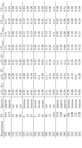
anisms of interval timing and provide constraints on current timing models. Table 1 collates the results from the major studies in the literature that have examined the statistics of these four variables. When possible we have sepa-rated the data by FI duration and, in only one case, also by reward magnitude. We did this because in a few cases the correlations were reported to be

signif-105

icantly different as a function of FI duration [23] and reward magnitude [24], although this was not the norm. Of particular note are the coefficients of vari-ation of each variable and their correlvari-ations. Note the strong similarity in the correlation patterns across 4 different species. The key results are as follows:

1. Positive correlation between start (S1) and stop (S2): ρ(S1, S2)>0;

110

2. Negative correlation between start and duration (D): ρ(S1, D)<0;

3. Positive correlation between duration and middle (M): ρ(D, M)>0;

4. Coefficient of variation (CV) for the start larger than for stop: CVstart>

(6)

The correlation results above mean that, in general, start times that occur

115

early/late into the trial are usually followed by early/late stops. In contrast, the duration of the period of high frequency responding tends to decrease with late starts and increase with early starts. Also, the coefficient of variation (CV =σ/µ) is larger for starts than for stops.

The four properties above will be referred to as thestationaryfeatures of the

120

peak procedure, to differentiate from thedynamic features related to learning when to stop when peak trials are first introduced. Existing timing theories do contend with some of this static data. SET can capture the first three features through the variance in its clock and memory processes [31] as can the TD(λ) algorithm coupled with a neural net function approximator [32]. The Multiple

125

Time Scales model [5] has the capacity to generate start and stop responses, but it is unclear whether that model can fit the full range of these timing features. Finally, BeT can be made to explain the correlation patterns if it is modified to include a variable transitional period when behavior switches (Gibbon and Church [31] called this modification the quasi-serial model, whilst Killeen and

130

Fetterman [33] called it augmented BeT). As Church, Meck and Gibbon [12] showed, however, this model is incompatible with correlations observed between subjects which SET can explain. It remains an open question whether other timing theories can accommodate these features.

Given the formal similarity between BeT and the TDDM [9], this raises

135

significant doubt as to whether the TDDM can be made to accommodate these trial-by-trial properties of the peak procedure. Below, the main formulation of the TDDM is briefly reviewed and then a new simplified version of TDDM’s stationary properties is introduced which allows for the derivation of the four static properties above analytically. The parameters thus obtained with the

140

simplified version are used with the full TDDM formulation; these simulations show that the results match appropriately.

2. Theory

2.1. The Time-adaptive Drift-diffusion Model (TDDM)

The drift-diffusion foundation of the TDDM is given by the stochastic

dif-145

ferential equation:

dx=A·dt+m·√A·dW (1)

whereA >0 is the drift or slope and m >0 is a constant that determines the amount of Gaussian white noisedW. Note that limiting Ato be positive and scaling the noise by√Aare particular to the TDDM, not to DDMs in general. In decision models, x(t) represents the current level of evidence toward a

150

(7)

Noisy evidence (noisedWand input evidenceAin equation (1)) are accumulated

155

by pushingxtoward one conclusion or the other.

Similarly, in the TDDM the accumulation process gathers noisy evidence that time has elapsed withA >0 andx≥0 [17, 16]. A single thresholdz >0 is used to mark the expected level ofxat the timeTof a salient event, a reward for example, such thatxcrosseszat timet=T on average. The time it takes forx

160

to reachz (sinceA >0, this will eventually occur) represents the psychological or subjective estimate for a given time interval. Moreover, because the noise

dW onxat every time step is Gaussian, the distribution of timestit takes for

xto reachz, which is the inverse, is given by the inverse Gaussian distribution [9]:

165

p

t; z

A, z2 m2_A

= z

m√At3₂_πexp

₋₍_At₋_z₎2

2Am2_t

(2)

with meanµ=z/Aand variance σ2=m2z/A2. In the TDDM, different time intervals are learned by adapting the drift rate A while holding the threshold

z fixed, such that A → z/T. Therefore, A can be seen as the rate at which the time interval is elapsing. It is the time-adaptability of A combined with the√A factor in equation (1) that differentiates TDDM from DDM, and that

170

gives TDDM its timescale invariance property [9]. If the events to be timed are unit-size rewards, thanAis equivalent to a reward rate.

The coefficient of variation of the time estimate produced by the TDDM is solely a function of the noisem and threshold z, and can be derived directly from the distribution (2):

CVTDDM= m √

z. (3)

Finally, equation (1) can be approximated numerically as

X(t+ ∆t) =X(t) +A·∆t+m·√A·∆t· N(0,1). (4)

The time-adaptive property of TDDM comes from slopeA taking the form of an exponential moving harmonic average of the observed intervals (Theorem 2 in[17]):

An+1= (1−α)An+α

1 ˆ

In

(5)

where ˆIn is the estimated time interval observed on thenth trial and 0< α≤1

is the learning rate. Without loss of generality, if z = 1, then at the time of reward (t = T), the value of X(t) (which must then be positive) produces a positive estimate ˆIn=Xn(T)/An of the time intervalT. The application of the

learning rule, when the cue indicating the end of the interval is observed, thus changes the slope A toward the inverse of this new perceived interval ˆIn such

that:

An+1= (1−α)An+α

An

Xn(T)

(8)

Given each trial begins withX(0) = 0, it can be seen that intervals perceived to be longer than T (with Xn(T) > 1) will decrease the rate A toward the

inverse of ˆIn > 0, while intervals perceived shorter than T (with Xn(T) <1)

175

will increase it. We refer the interested reader to [17] and [9] for a full exposition of the learning rules at the real-time (time-step) level. In the case of the peak procedure, where the intervals are always of the same duration, equations (4) and (6) are the only ones needed.

Note that in the peak procedure, we assume the learning rule is only applied

180

when the reward occurs. As a result, there are no updates to the rate A on peak trials. In line with this assumption, some experiments have reported that peak trials have little or no impact on the start and stop times [20, 21], but others have reported a leftward shift of the response curve following peak trials [12] (but no relationship with peak-trial duration). This latter finding suggests

185

some influence of peak trials on later trials, but this effect would not seem to be mediated by an update of the memory for time as encoded in the drift rateA. Any update due to the long peak trials should actually induce later responding and a right-ward shift of the response curve (opposite to that observed). Instead, this finding probably reflects an incomplete reset of the accumulator following

190

peak trials.

2.2. Application of the TDDM to the peak procedure

As suggested by [9], perhaps the simplest way to account for the abrupt switch back to a low response rate in individual trials of the peak procedure is to use two thresholdsz1< z2. The first thresholdz1marks the time to start the high response rate, and the second threshold z2 marks the time to stop. This modification would immediately produce the difference in the CV for starts and stops (feature #4) because by (3)

CVstart= m √

z1 >√m

z2

= CVstop.

Note that feature #4 rules out the possibility of having two consecutive single-threshold timers (one determining the start time, and one determining the stop time), because starting the second timer when the first one reaches a

195

threshold would force CVstop ≥CVstart. Similarly, having two parallel

single-threshold timers would break feature #1 by producing ρ(S1, S2) = 0, unless there is really only one timer, or unless some extra common factor is added. Thus, the single-timer two-threshold approach seems the most sensible option available. The mechanism for the emergence of such a second threshold

dur-200

ing training remains unknown, but for the current purpose of explaining the stationary features of the peak procedure, we need only to assume its existence. Due to TDDM’s learning ability, however, it is not immediately clear what other modifications would be needed in order for the model to exhibit the four stationary properties of the peak data. Many variations on the model could

205

(9)

space, we built a simplified version of the TDDM without noise in the diffusion process (i.e. settingm = 0 in equation (4)) and without applying the slope-adaptation rules (equation (6)) directly. Instead, we propose to approximate

210

the stationary distribution of the slope A as a result of these two interacting components.

2.3. TDDM: A simplified formulation

The learning rule for adaptingAin equation (6) can be seen as a Robbins-Monro algorithm [34], which estimates the reward rate (assuming fixed unit-size

215

rewards) for the stimulus on non-peak trials. The slopeAn is therefore an

im-proving estimate of the reward rate given the noisy measure ˆIn =X(T)/An of

the true time interval T provided by the accumulator at the time of reward. This algorithm, under some conditions, converges by the law of large numbers to a normal distribution centered on the reward rate. Under steady-state

con-220

ditions, we can therefore approximate the full model by replacing the noise

min the accumulation or memory process and the application of the learning rule altogether by sampling the slopeAn at the beginning of each trial from a

Gaussian distributionN(z/T, σ2) clipped above 0.

Sampling the slope A produces a range of values across trials. On trials

225

when the slope is high, both start and stop times are low; on trials when the slope is low, both start and stop times are high. As a result, there is a positive correlation across trials (feature #1, see Fig. 2). This sampling, however, is insufficient to generate a negative correlation between the start and the duration (feature #2).

230

As shown on the simplified TDDM diagram in Fig. 2, a simple way to account for the negative correlation while maintaining CVstart >CVstop (feature #4)

is to add noise to the start threshold z1. At the beginning of each trial, a threshold Z1,n is sampled from a probability distribution with a given mean

and variance (for simplicity we used a uniform distributionU(a, b) whereaand

235

b are estimated from the data but in principle other distributions could have been used instead). Note that this increases the CVstartto which equation (3)

does not apply anymore, while maintaining feature #4. On trials when the sampled threshold is low, the start time will be low and the duration high, while the opposite will happen when the threshold is high, giving rise to a

240

negative correlation between the start time and the high response rate duration (feature #2, see Fig. 2).

Note that adding noise to the stop threshold instead of the start threshold would not be sufficient to fit the data. It would increase the CVstop, which

may then require additional noise in the start threshold to maintain feature #4

245

(CVstart>CVstop). Thus, although adding noise to the stop threshold is also

possible, adding noise only to the start threshold is simpler (and as we will show, appears to be sufficient).

A major advantage of this simplified formulation is that it allows a direct analytic derivation of estimates for the model parameters in the full TDDM

250

(10)

[image:10.612.136.463.137.313.2]

Figure 2: Diagram illustrating how the correlations seen in the data can be derived from the simplified model. The panels show two hypothetical trials: the left with a low slope

Aand the right with a high slope A. This variable slope induces a positive correlation betweenS1andS2, and betweenD andM. To highlight the effect of the noise in threshold z1, two corresponding valuesS1 are shown (minimum and maximum) on each panel, with

their corresponding durations and middle points. This noisy threshold induces a negative correlation betweenS1andD.

be used to directly generate predictions for the correlations. Secondly, it will be used to estimate most parameters of the full model directly from the same CVs. The full model will then be simulated to produce predictions for these

255

same correlations, and to asses the degree of agreement between the data, the simplified model, and the full model. Finally, the simplified model will also be mapped to SET. Thus, the simplified model will provide a link between the CVs and the correlations, as well as between the full model and SET under stationary conditions.

260

3. Results

3.1. Simplified TDDM

Let S1, S2, M and D be the times of start time, stop time, middle and duration respectively with start and stop thresholds Z1 and z2 respectively. Then according to the simplified model:

S1= Z1

A, M =

S1+S2

2 =

Z1+z2

2A ,

S2= z2

A, D=S2−S1=

(11)

LetZ1and 1/Abe independent random variables with meansE(Z1),E(1/A) and variancesσ2_Z

1,σ 2

1/Arespectively. It is then possible to write all the statistics

of the peak procedure in terms of the squared coefficients of variation ofZ1and

265

1/A, γ_Z2₁ and γ₁2_/A respectively, and the ratio of the thresholds θ =z2/E(Z1) (see supplementary material for the complete mathematical derivations of these statistics). The squared coefficients of variation are:

γ_S2 1=γ

2 1/A+γ

2

Z1·γ 2 1/A+γ

2

Z1, (7)

γ_S2₂=γ₁2_/A, (8)

γ_D2 = γ

2

Z1(1 +γ 2 1/A)

(θ−1)2 +γ 2

1/A, (9)

γ_M2 = γ

2

Z1(1 +γ 2 1/A)

(θ+ 1)2 +γ 2

1/A. (10)

The correlations are:

ρ(S1, S2) =

1

r

γ2

Z1+

γ2 Z1

·γ2 1/A

+ 1

, (11)

ρ(S1, D) =

γ2

1/A(θ−1−γ

2

Z1)−γ 2

Z1 q

γ2 1/A(γ

2

Z1+ 1) +γ 2

Z1· q

γ2

1/A[(θ−1)2+γ

2

Z1] +γ 2

Z1

, (12)

ρ(D, M) = γ

2 1/A(θ

2₋₁₋_γ2

Z1)−γ 2

Z1 q

γ2

1/A[(θ+ 1)2+γ

2

Z1] +γ 2

Z1· q

γ2

1/A[(θ−1)2+γ

2

Z1] +γ 2

Z1 . (13)

We can demonstrate that a constant start threshold z1, as opposed to a

270

stochastic threshold, is qualitatively inconsistent with the data. Ifz1is constant,

thenγ2

z1= 0, which when substituted into equations (11) to (13) yields positive

correlations for all three cases, contrary to the data:

ρ(S1, S2) =

1

√

0 + 0 + 1 = 1,

ρ(S1, D) =

γ2

1/A(θ−1)

q

γ2 1/A·

q

γ2

1/A(θ−1)2

=

γ2

1/A(θ−1)

γ2

1/A(θ−1)

= 1,

ρ(D, M) = γ

2 1/A(θ

2₋₁₎

q

γ2

1/A(θ+ 1)2·

q

γ2

1/A(θ−1)2

= 1.

(12)

of variation or the correlations. It is simpler to use the coefficients of variation (7)-(10):

γ1/A=γS2 (14)

γZ1= s

γ2

S1−γ 2

S2

1 +γ2

S2

(15)

θ=



  

  

1 +

r

γ2 S1−γ

2 S2

γ2 D−γ

2 S2

if using (9)

−1 +

r

γ2 S1−γ

2 S2

γ2 M−γ2S2

if using (10)

(16)

The equations above show that, with the simplified TDDM, three pieces of information from the data, namely the coefficients of variation of start, stop and

275

[image:12.612.202.482.490.671.2]

either middle or duration, are sufficient to determine the three correlations in Table 1.

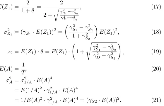
Although not necessary to find the correlations, one could simulate (or sam-ple) the simplified TDDM using the same three CVs to determine its five pa-rameters, which are the mean start threshold E(z1), stop thresholdz2, mean

280

accumulator slopeE(A), start threshold variance σ_Z2₁, and slope variance σ_A2. In setting these parameters we have assumed without losing generality that the accumulator aimed at hitting a thresholdz= 1 at the time of reinforcement, and that the two thresholds to start and stop responding are set so as to surround the reinforcement threshold: (E(Z1) +z2)/2 = 1. This assumption implies that the

285

midpointM of high frequency responding is exactly in the middle of start and stop, something that is roughly true (see Table 1 in [12]). Usingθ=z2/E(Z1),

it follows thatz2=θ·E(Z1) andE(Z1) = 2/(1 +θ). The five simplified TDDM

parameters, can be expressed directly in terms of data, namely the three CVs (CVstart=γS1, CVstop=γS2, and CVdur=γD), as follows:

290

E(Z1) = 2 1 +θ =

2

2 +

r

γ2 S1−γ

2 S2

γ2 D−γ2S2

, (17)

σZ21 = (γZ1·E(Z1)) 2

=

_γ2

S1−γ 2

S2

1 +γ2

S2

E(Z1)2, (18)

z2=E(Z1)·θ=E(Z1)· 1 +

s

γ2

S1−γ 2

S2 γ2

D−γ

2

S2 !

, (19)

E(A) = 1

T, (20)

σ_A2 =σ₁2_/A·E(A)4

=E(1/A)2·γ₁2_/A·E(A)4

(13)

In derivingσ_A2 we made use of the Taylor approximationσ₁2_/A≈E(A)−4·σ_A2

(see Appendix D). In the case ofθ, if both CVmidand CVdurare available from

the data we have a choice between which one to use (see equation (16)). We have used θ derived from CVdur in all models because this value provided a

better agreement with the data, probably because it conveys information about

295

the anti-correlated noise between the start and stop which is filtered out in the middle point. Notice that the correlation equations (11) to (16) do not take as input the interstimulus intervalT of the FI trials, which is coded in the variable 1/A; making the correlations completely independent of the FI timescale in this model. The estimates for the five simplified TDDM parameters are calculated

300

with equations (17) to (21) based on the three CVs from the data.

The correlations derived from the simplified TDDM can be found under the column Simp. in Table 2. Because the model takes as input the coefficients of variation for start, stop and duration, we were not able to model the two studies [22, 25] that did not report these variables. Out of the 19 experiments

305

left, only two violated constraints imposed by the model. The data with FI 5 seconds in [23] has γ2

D = γ2S2 which causes the denominator in the radical in

equation (19) (stop threshold) to be zero. The data in [24] for FI 17 seconds and LOW reward hasγ_S2₂> γ_S2₁which generates imaginary values for the start (equation (17)) and stop (equation (19)) thresholds. Therefore we did not report

310

the correlations produced by the models for these two experiments.

In some cases, one or more correlations were not reported in the original paper (marked as n/a in Table 2), so in these cases results are provided as pre-dictions only. Considering all 44 correlations available out of the 17 experiments with the appropriate CVs pattern, the model’s correlations deviate by 0.09 on

315

average from the correlations in the data, with the worst case beingρ(S1, S2) in

[24] for FI 10H (see also Figure 3, first bar of each plot). In five cases (out of 51) the model generates the wrong correlation sign, but those values are very close to zero (≤0.03, marked by an * in Table 2), and two of them are not available in the animal data to be verified. Such very small, wrong-signed, correlations

320

can also be observed in [24] for FI 17 seconds and LOW for ρ(S1, D). In gen-eral, such small correlations are not robust enough to be clearly considered of a specific sign. Overall, using only three pieces of information from the data the simplified model reproduces the pattern of correlations generally well and generates values similar to the data in most cases as shown on the left-most bar

325

of each plot in Figure 3.

3.2. Full TDDM

The full model (equations (4) and (6)) was then simulated assuming learning occurs only on rewarded trials (andXn(0) = 0 at the beginning of each trial).

Peak and rewarded trials were randomly generated following the proportions

330

(14)

[image:14.612.161.445.123.227.2]

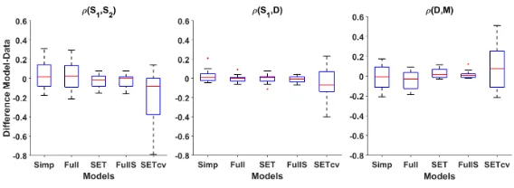
Figure 3: Box-plot of the differences in correlations between the animal data and each model for all 16 experiments to which the simplified TDDM can be fit. Each plot represents, from left to right: the simplified TDDM (Simp), the full TDDM using the same parameters val-ues (Full), SET fit to the correlations (SET), the full TDDM using parameters from SET (FullS), and SET fit using only the same 3 CVs as the simplified model (SETcv). In short, the simplified model and SET can both provide good estimates of their equivalent TDDM on stationary conditions. Though SET gets lower error on correlations than the simplified TDDM, it does so at the cost of error on CVs. SET, however, is not as good as the simplified model at predicting the correlations from CVs only (last column of each sub-plot).

rule aims at thresholdz= 1 when the reward occurs. The slope was initialized

335

with the exact value A = 1/T. The only remaining free parameter was the learning rateα. For each experiment, and each α∈ {0,0.05,0.10, ...,1.00}, we ran 30 simulations of 1000 trials each, to gather means and standard deviations for each measure of interest, namely the 4 CVs and the 3 correlations.

The best matching correlation triplets derived from the full TDDM can be

340

found under the columnFull in Table 2. Considering all 44 correlations avail-able out of the 17 experiments with the appropriate CVs pattern, the model’s correlations deviate only by 0.08 on average from the correlations in the data, with the worst case being againρ(S1, S2) in [24] for FI 10H. The simulations did not generate the wrong correlation sign on average, except for 1 experiment

345

from [30], where the model predictsρ(D, M)≈ −0.02, but the real value is un-known. As shown in Table 2, the correlations are quite similar, across all results (animal, simp. TDDM, and full TDDM). Despite only one wrong correlation sign (as opposed to five for the simplified model) out of 51, the full TDDM gives very similar results to the simplified TDDM on this task. As shown in Figure

350

3 (two first bars of each plot), the distribution of errors is very similar for both models. Moreover, on average, the absolute difference between a correlation in the simplified model and the full model is 0.04. These results show that the simplified model is a good approximation of the full model under stationary conditions. In addition, the extra learning parameter in the full model is shown

355

to be of little use in explaining the current datasets on the intra-trial structure of responding on the peak procedure. This outcome is as expected because the extra learning rate parameter in the TDDM should play an important role mostly when learning new intervals, but is expected to have little impact on stationary behaviours.

360

(15)

on the CVs between the original data and the CVs produced by the simulations of the full TDDM. The average absolute CV error was 0.08 with the worst case being 0.17 in [24] for FI 10H, CVdur. This discrepancy, albeit small, is most

likely due to the setting ofm=γ1/A, asγ1/A represents a mixture of perceptual

365

noise mand the learning rate α. Whether there could be an analytic formula to set those parameters (m and α) remains an open question. The full model has an extra degree of freedom in the learning rateα, but to properly estimate this balance betweenmandαwould require additional information about the learning dynamics, before steady-state occurs. In the simplified model, γ1/A

370

mergesmandαparameters from the full model, and this issue does not arise. Nonetheless, we can still estimate the learning rate, which across all 17 experi-ments was consistently high and ranged between 0.45 and 0.85 (with a median of 0.70). Moreover, in about 9 of the 16 experiments for whichαhas been opti-mized (for [28], we used the median 0.70 since no correlations were available), a

375

small learning rate could adversely impact the sign ofρ(D, M). A high TDDM learning rate was also found to best fit a different timing task in [18], suggesting that a high learning rate may be necessary, even when learning is not directly observable.

To further investigate this hypothesis, we measured the correlation between

380

the perceived time estimate of the model (provided by 1/Xn(T)) on reward

tri-als preceding peak tritri-als and the stop time of the subsequent peak tritri-als. The average correlation across all 17 experiments was 0.61, as expected from such a high learning rate (e.g., forα= 0.7, the last 2 trials account for 91% of the mem-orized interval). Unfortunately, it might be challenging to measure an animal’s

385

perceived time estimate for a single trial to see such trial-to-trial correlations in behaviour. Another possibility would thus be to slightly change the rewarded interval on those pre-peak reward trials to generate enough measurable changes in responding on the subsequent peak trials. We found that varying those in-tervals using 1.33 times the CV was sufficient to produce a correlation between

390

one reward trial’s intervals and the following peak trials stop times for all 17 experiments (generating a correlation> .47 across all experiments with a mean of 0.61). For example, if the FI is 20s and the CVstop = 0.15, then using

pre-peak trial intervals of 16s and 24s should be enough to detect a learning effect. This prediction remains to be tested in animals.

395

Finally, as an illustration that the TDDM can produce similar average curves seen in the data, Fig. 4 shows an example of how the model predicts the start and stop times on each trial and how averaging these times produces the peak in response rate around the time of reinforcement.

3.3. Relationship with SET

400

An important further observation is that the simplified TDDM presented above is formally equivalent to a constrained version of the two-threshold version of SET developed for the peak procedure in [12].

SET incorporates 4 components: a clock (or accumulator), a memory of reinforcement times, a source of noise, and a comparator. Originally, the

accu-405

(16)

[image:16.612.165.437.133.293.2]

Figure 4: TDDM simulation using parameters derived from data in [35]. Left plot: start and stop times for each peak trial. Right plot: averaging over all trials produces the peak of response frequency seen in data.

was removed in more modern versions (either because it was unnecessary or be-cause it would break timescale invariance [36, 5]). Thus, SET has a noise-free accumulatorn representing theperfectestimate of elapsed time in the current trial. The memory is the memory of reinforcement times. It is represented as

410

a distribution determined by an expected value and a coefficient of variation providing across-trial variability and timescale invariance. At the beginning of each trial, a samplen∗ is generated from the memory and used for comparison with the accumulated running timen. There is finally a comparison threshold

bsuch that the animal starts responding when the ration/(n∗·k∗)> b, where

415

k∗ is a multiplicative noise source, which could easily be interpreted as related to clock speed (k∗ is usually introduced before saving the time to memory in SET, but this aspect is not important here).

For the peak procedure, a second threshold was introduced for the stop time in [12]. Because an extra source of noise was necessary to explain the trial

420

statistics, two stochastic thresholds were used, l = 1−b1 and and u= 1 +b2

(each having a mean and variance). Thus, the model starts responding a short time before the remembered interval and stops a short time after. Note that the single threshold in the original version of SET was considered constant. Adding noise to the start threshold is necessary to get the pattern of

inter-425

trial correlations discussed here, but the simplified TDDM results suggest that noise in the second threshold is not necessary. The expected value of the time memory is assumed to come from experience and is therefore fixed by the task. The remaining parameter of the model is the CV of that memoryγ (k∗ is not mentioned in [12]).

430

(17)

there are two sources of noise generating trial-to-trial variability because the start thresholdz1 was regarded as a constant. The first source comes from the accumulator, in the termm·√A·dW in equation (1). The drift rateA= 1/T

435

encodes the interval memory, and the√Afactor generates timescale invariance on reading rate A. The second source of noise comes from trial-to-trial vari-ability in A due to the learning rule in equation (6). These two sources of variability are merged together in the simplified TDDM in the distribution of

Anwhich uses the trained interval as its expected value. ThusAnin the

simpli-440

fied TDDM is equivalent to SET’sn∗ memory, except thatAn represents rates

whilen∗represents durations.

In adapting the TDDM to the peak procedure data, we found that it was analytically sufficient to add noise only into the start threshold (noise in the stop threshold can be added, but must remain smaller than in the start threshold).

445

Thus, while in [12] SET uses two noisy thresholds, the simplified TDDM shows that a noisy start threshold and a fixed stop threshold are sufficient to explain the data. Moreover, SET allows for full fitting of the two threshold positions (in terms of proportion of time interval). Because the CVs themselves cannot give threshold locations, but only some information about their relative time

450

positions, we use the fact that the peak response is near the FI to estimate a threshold ratioθand locate the thresholds on both sides of it. Thus, the TDDM has only 3 parameters directly estimated from specific measurements (3 CVs) whereas SET requires a search process to optimize its 5 parameters. Beyond that, the thresholds in SET and the simplified TDDM are the same.

455

The key equations of the simplified TDDM (Equations (7) to (13)) are equiv-alent to the two-threshold SET equations in Fig. 13 in [12]. Table 3 further shows the correspondence between SET and the simplified TDDM in terms of their parameters. As an example, we show how SET’s formula for the coefficient of variation of the middle time (cv(m) in Fig. 13 in [12] is equivalent toγM in

the Simplifed TDDM):

γ₊2 = σ

2

u+σ

2

l

(U+L)2 = σ2

z2+σ 2

Z1

(z2+E(Z1))2 =

σ2

Z1

(θE(Z1) +E(Z1))2 =

σ2

Z1 E(Z1)2₍_θ_{+ 1)}2

= γ

2

z1

(θ+ 1)2.

cv2(m) =γ2(1 +γ₊2(1 +γ−2))

=γ2+γ₊2γ2+γ₊2 =γ2₁_/A+ γ

2

Z1

(θ+ 1)2γ 2 1/A+

γ2

Z1

(θ+ 1)2

=γ

2

Z1(1 +γ 2 1/A)

(θ+ 1)2 +γ 2 1/A=γ

2

M,

becauseσ2

z2 = 0 as we assume here thatz2is constant. The other six equations

in Fig. 13 in [12] can be transformed into the notation from the simplified TDDM in a similar manner.

To quantitatively compare SET and the simplified TDDM, we implemented SET and, using a grid search, found the parameters that best fit the 3

(18)

tions for each experiment. In the grid search, the mean memory time was the FI, the CV could vary from 0.05 to 0.25, the largest CV, by steps of .05, the two thresholds could vary from .1 to .9 by steps of .1 on each side of the FI indepen-dently, and their standard deviations could vary from 0.00 to 0.75−CVparam value

and 0.25−CVparam value for the start and stop threshold respectively, where

465

CVparam value was the value of the CV parameter for a given grid point. In

the simulations, if the memory time or start threshold where negative or if the stop threshold was smaller than start threshold, these were then resampled. If a given set of parameters generated 10% or more of such invalid values, that set of parameters was skipped.) A total of 30 simulations of 1000 trials each were

470

run for every grid point (as in the full TDDM). The mean absolute error on all available correlations for all 17 experiments TDDM could fit was 0.05 (as op-posed to 0.09 for the simplified model), and there was no sign error (comparing the first and third bars on each plot of Figure 3).

The absolute difference in parameters value between the two models is

pro-475

vided in the last column of Table 3. The noise levels were very close to each other, including the stop threshold. The main difference was in the extra free-dom SET has to position the start and stop thresholds relative to the FI. This error reduction, however, came at a cost. SET has 2 extra parameters and the fitting used all 7 pieces of information available, compared to the simplified

480

model that only used 3. Whereas the simplified model used the exact CVs, SET produced substantial error on each of them (0.04 on average, for each CV). Thus, the reduced error on the correlations was counteracted by increased error on the CVs. When fitting SET using only the same 3 CVs as the simplified TDDM, SET’s absolute error on correlations increased from 0.05 to 0.19 (more

485

than double the simplified model, see the last bars of each plot on Figure 3 as compared to the third bars). Thus, SET has a little less predictive power, but the discrepancy between the SET and TDDM thresholds would be better analysed by looking at the start and stop temporal positions relative to the FI in future studies.

490

To further assess whether SET (like the simplified model) could be used as an estimate of the full TDDM under stationary behaviours, we augmented the full TDDM to support two thresholds with specific means and variances. We then ran the same simulations as before, but feeding the SET parameters directly into this augmented TDDM as estimates (usingm=γ and optimizing αto match

495

the correlation as before). The average absolute error for this augmented full TDDM average was 0.04 (as opposed to 0.05 for SET alone, comparing the third and fourth bars on each plot of Figure 3), and the average absolute difference in correlation between SET and its TDDM equivalent was 0.03 (as opposed to 0.04 for the simplified TDDM and its full equivalent). The learning rate was also

500

similar to the previous TDDM simulations with α ≥0.55 for all experiments with a median of 0.90, thus confirming the prediction about sequential effects made in the previous section. In short, the TDDM, although well-known for modelling the learning dynamics, can be well approximated by SET (with the same parameters) under stationary conditions.

505

(19)

and SET, as well as having showed that they can both serve to provide estimates for the parameters for their TDDM equivalent under stationary conditions. The simplified TDDM model provides a way to show that adding noise in the start threshold and having a fixed stop threshold is sufficient for the full TDDM to

510

fully account for the micro-structure of peak-interval data, and to link SET to the TDDM under stationary conditions without removing the TDDM’s ability to also reproduce trial-to-trial time learning dynamics [18, 16]. Moreover, the formulae developed to estimate the TDDM’s parameters can also be turned into formulae to estimate SET’s parameters directly from the CVs, without the need

515

to run thousands of simulations to find the best possible parameters (as in [12]). While SET can also be used as an estimate of the full TDDM for stationary conditions, a major advantage of the full TDDM over SET is that it is not limited to stationary behaviours, as it also covers time-adaptive phenomena through its learning rule.

520

4. Discussion

This paper extends the TDDM to deal with the micro-structure of respond-ing on the peak procedure, when rewards are occasionally omitted. A simplified version of the TDDM was introduced, which allows for analytic derivation of model predictions for steady-state behaviour. This simplified version is also

525

shown to be equivalent to a constrained version of Scalar Expectancy Theory, making SET a special case of the broader drift-diffusion framework.

This paper also provides, to the best of our knowledge, the most comprehen-sive review of single-trial analyses in the peak procedure, which reveals a con-sistent pattern of correlations and CVs observable in the trial micro-structure

530

across 19 of 21 data sets. The TDDM and its simplified model were both able to provide good fits for most correlations available as well as to make realistic predictions for those which were not, such as in [28]. The two cases in which they both failed to fit the data—FI 5 in [23] and FIs 17L in [24]—were in direct violation of the model’s constraints imposed by equations 15 and 16 (the data

535

had eitherγ_S2₂ > γ_D2 orγ2_S₂ > γ_S2₁). In a few cases the simplified model had the wrong sign, but those predictions were too close to zero for the sign to be clear and in some of those cases, the experimental correlations were not available.

The TDDM, in its original formulation, could be expanded in many different ways to fit the peak procedure data. For example, multiple accumulators, in

540

parallel, or in sequence, could be used to determine when to start and to stop, with each potentially having different noise factors, thresholds, and learning rates. Given that using distinct timers for the start and stop could easily be eliminated, we developed an approximation or simplified model of the TDDM using a single timer for steady-state or stationary behaviours. We then used

545

it to find the simplest modifications that could account for the peak procedure statistics. By adding to this simplified TDDM an extra threshold to account for the stop time on peak trials and noise to the start time threshold, we were able to generate predictions that fit the data well. Simulations using the full TDDM formulation corroborated the simplified TDDM results and also validated the

(20)

simplified version as a good approximation of the full TDDM’s steady-state behaviours. Thus, in future studies, this simplified version can be useful in formulating hypothesis and generating parameters that can later be tested with the full TDDM.

The paper also demonstrates that this simplified TDDM is formally

equiv-555

alent to a specific version of SET on many tasks covered by SET. Therefore, a direct comparison between these two models could be made. Although math-ematically equivalent, there are possible differences in interpretation. For ex-ample, SET postulates a Poisson pacemaker but this feature does not influence timing noise, because, within SET the error in reading and writing in memory

560

overcomes the Poisson variability. In the TDDM, the Poisson noise resides in the opponent-process underlying the noise m in the DDM [18]. That DDM noise can be considered both the error in reading the slope value at every time step [17] as well as perceptual error generated by this accumulation of noise. This error, combined with the learning process, seems sufficient to explain the

565

inter-trial variability covered in SET by the memory error. Finally, though SET works in steady-state tasks such as the peak procedure, the theory has no possible mechanism to account for any learning dynamics. While we showed that SET can be used to estimate the full TDDM (or its parameters), the full TDDM on the other hand, can adapt its drift rate to also account for behaviour

570

on dynamic tasks, as previously demonstrated in the case of random and cyclic schedules of reinforcement [18, 16]. This adaptive element may also predict hitherto unreported effects. Depending on the values chosen forαand m, the full TDDM could show sequential trial-to-trial dependencies by appropriate ma-nipulation of the FI on reward trials preceding peak trials. A deeper account

575

of such sequential effects would require data from the beginning of training to setαandm more precisely, but some testable predictions were made with the model assumingαstays high (≥0.5).

While the question of whether there is one central clock or a bunch of dis-tributed timers in the brain is still debated [37], SET usually posits a central

580

clock, whereas the TDDM does not require such a central pacemaker and could very well suppose different accumulators for each interval being timed. The data from [23] also contains an experiment looking at the timing of multiple durations, which could pose a challenge to such a multiple timers idea. In one experiment, 3 distinct durations were used, allowing evaluation of the start and stop times

585

for the different timed durations in the same peak trial. Interestingly, they found that stop times for the different durations were correlated within trials, suggesting a common clock noise (in SET), which would go against having the 3 different intervals in 3 different integrator rates for the TDDM. There is, how-ever, also evidence that diffuse neurotransmitters, such as dopamine [38], can

590

influence time perception. Thus, in a multiple-duration procedure, dopamine might diffusely influence all the timers in parallel. In the TDDM, this could be modelled by adding a commonkfactor in front of Ain equation (1), affecting all timers speed equally. Such a parameter could also be considered equivalent to SET’s k∗ parameter and could be added to the simplified model as well,

595

(21)

It would be necessary to develop formulae to isolate the variability ofk across trials from the other sources of noise, possibly from the stop time correlation in the multiple duration trials. This is beyond the scope of this paper.

The TDDM also provides a degree of neural plausibility that most other

600

timing models lack. For example, Simen et al. [18] showed how the TDDM could be represented at a lower level by a pool of Poisson firing neurons, even at long multi-second timescales [18, 39]. In addition, neurons with climbing activity which adapt their climbing rate to the necessary delay (exactly like TDDM) have already been recorded in numerous brain areas over short timescales, such as the

605

thalamus (adapting between 1- to 2-s intervals) [40], the posterior parietal cortex (adapting between 300ms and 800ms intervals) [41], and in the inferotemporal cortex (adapting between 4 and 8 seconds intervals) [42].

The TDDM, however, can reproduce adaptive behavioural data on timescales up to 90 s and technically should work on static data for any timescale —not

610

only the shorter timescales above. Recent work by Mello et al. [43] fills this gap in the timescale of the neural substrate. They found evidence for an adaptive neural representation in the striatum, which changes for intervals varying from 12 to 60 s. In rats performing a timing task, neurons from a pool of striatal neurons fired in sequence with each neuron roughly representing a different

615

elapsed time. When the time interval was changed, this neural representation adapted to the interval duration, with the same neuron representing a similar relative time, but different absolute time. Such a dynamic adjustment of the time scale is a fundamental element of the TDDM, but lies outside the scope of SET’s static representation.

620

The adaptive nature of the neural representation also does not accord with most learning models of timing which assume a fixed and predetermined time-code [5, 6, 7, 8]. An important outstanding question is how a population of spiking neurons such as the one found [43] could implement the learning rule as defined in equation (5) from [18, 17]. Nonetheless, the TDDM is perhaps unique

625

among timing models to incorporate an adaptive representation of elapsed time, in accordance with the neural data, and to still fit the behavioural data under static conditions. Therefore, the TDDM seems well positioned as a simple high-level model that also accurately express lower-high-level neural representations.

One particularly appealing feature of the TDDM is the breadth of situations

630

to which similar DDM formalisms can be applied. Whereas SET is a dedicated timing model, the TDDM is a model based on some of the same principles of the more general drift-diffusion class of models, which are well established in decision making and encounter wide physiological support [44, 14]. Though the computations are not strictly identical, in that the drift rate is adaptively scaled

635

(22)

References

640

[1] C. V. Buhusi, W. H. Meck, What makes us tick? Functional and neural mechanisms of interval timing., Nature Reviews Neuroscience 6 (10) (2005) 755–765.

URL http://eutils.ncbi.nlm.nih.gov/entrez/eutils/elink. fcgi?dbfrom=pubmed{&}id=16163383{&}retmode=ref{&}cmd=

645

prlinkspapers2://publication/doi/10.1038/nrn1764

[2] S. Grondin, Timing and time perception: a review of recent behavioral and neuroscience findings and theoretical directions., Attention, perception & psychophysics 72 (3) (2010) 561–582.

URL http://eutils.ncbi.nlm.nih.gov/entrez/eutils/elink.

650

fcgi?dbfrom=pubmed{&}id=20348562{&}retmode=ref{&}cmd= prlinkspapers2://publication/doi/10.3758/APP.72.3.561

[3] J. Gibbon, Scalar expectancy theory and Weber’s law in animal timing, Psychological Review 84 (3) (1977) 279–325.

[4] P. R. Killeen, J. G. Fetterman, A behavioral theory of timing.,

Psycholog-655

ical Review 95 (2) (1988) 274–295.

URL http://eutils.ncbi.nlm.nih.gov/entrez/eutils/ elink.fcgi?dbfrom=pubmed{&}id=3375401{&}retmode=

ref{&}cmd=prlinkspapers2://publication/uuid/ 8D608E96-488C-470F-AD23-7F0A65FEF58C

660

[5] J. E. R. Staddon, J. J. Higa, Time and memory: towards a pacemaker-free theory of interval timing., Journal of the experimental analysis of behavior 71 (2) (1999) 215–251.

URL http://www.ncbi.nlm.nih.gov/pmc/

articles/PMC1284701/papers2://publication/uuid/

665

BDD2DD5B-324A-4E12-B7A6-B8A5964C5643

[6] S. Grossberg, N. A. Schmajuk, Neural dynamics of adaptive timing and temporal discrimination during associative learning, Neural Networks 2 (2) (1989) 79–102.

URL http://www.sciencedirect.com/science/article/pii/

670

0893608089900269papers2://publication/doi/doi:10.1016/ 0893-6080(89)90026-9

[7] E. A. Ludvig, R. S. Sutton, E. J. Kehoe, Stimulus representation and the timing of reward-prediction errors in models of the dopamine system., Neural computation 20 (12) (2008) 3034–3054.

675

prlinkspapers2://publication/doi/10.1162/neco.2008.11-07-654

[8] A. Machado, M. T. Malheiro, W. Erlhagen, Learning to Time: a per-spective., Journal of the experimental analysis of behavior 92 (3) (2009)

(23)

423–58. doi:10.1901/jeab.2009.92-423.

prlinkspapers2://publication/doi/10.1901/jeab.2009.

92-423http://www.pubmedcentral.nih.gov/articlerender.fcgi?

685

artid=2771665{&}tool=pmcentrez{&}rendertype=abstra

[9] P. Simen, F. Rivest, E. A. Ludvig, F. Balci, P. Killeen, Timescale Invari-ance in the Pacemaker-Accumulator Family of Timing Models, Timing & Time Perception 1 (2) (2013) 159–188.doi:10.1163/22134468-00002018. URL http://wrap.warwick.ac.uk/58690/http://booksandjournals.

690

brillonline.com/content/journals/10.1163/22134468-00002018

[10] S. Roberts, Isolation of an internal clock., Journal of Experimental Psy-chology: Animal Behavior Processes 7 (3) (1981) 242–268. doi:10.1037/ 0097-7403.7.3.242.

URL http://doi.apa.org/getdoi.cfm?doi=10.1037/0097-7403.7.3.

695

242

[11] A. Machado, Learning the temporal dynamics of behavior., Psychological Review 104 (2) (1997) 241–265.

700

ref{&}cmd=prlinkspapers2://publication/uuid/ 087AAE03-52E2-498A-8A18-92A70CE44EF5

[12] R. M. Church, W. H. Meck, J. Gibbon, Application of scalar timing theory to individual trials., Journal of Experimental Psychology: Animal Behavior Processes 20 (2) (1994) 135–155.

705

ref{&}cmd=prlinkspapers2://publication/uuid/ 5983C704-7A71-4F1A-89E9-4DACE7E601FE

[13] R. Ratcliff, A theory of memory retrieval., Psychological Review 85 (2)

710

(1978) 59.

URL http://psycnet.apa.org/journals/rev/85/2/59/papers2: //publication/uuid/C23DBAF7-0C7E-434A-8A3C-D9F0945328B8

[14] J. I. Gold, M. N. Shadlen, The neural basis of decision making., Annu. Rev. Neurosci. 30 (2007) 535–574.

715

prlinkspapers2://publication/doi/10.1146/annurev.neuro.29. 051605.113038

[15] A. Voss, M. Nagler, V. Lerche, Diffusion models in experimental

psychol-720

(24)

402. doi:10.1027/1618-3169/a000218.

URLhttp://www.ncbi.nlm.nih.gov/pubmed/23895923

[16] A. Luzardo, E. A. Ludvig, F. Rivest, An adaptive drift-diffusion model of interval timing dynamics, Behavioural Processes 95 (2013) 90–99.

725

doi:10.1016/j.beproc.2013.02.003.

URL http://www.ncbi.nlm.nih.gov/pubmed/23428705http: //linkinghub.elsevier.com/retrieve/pii/S0376635713000247

[17] F. Rivest, Y. Bengio, Adaptive Drift-Diffusion Process to Learn Time In-tervals, Arxiv preprint arXiv:1103.2382.

730

URLhttp://arxiv.org/abs/1103.2382

[18] P. Simen, F. Balci, L. de Souza, J. D. Cohen, P. Holmes, A model of interval timing by neural integration., The Journal of neuroscience : the official journal of the Society for Neuroscience 31 (25) (2011) 9238–9253.

doi:10.1523/JNEUROSCI.3121-10.2011.

735

[19] F. Balcı, P. Simen, Decision processes in temporal discrimination., Acta psychologicadoi:10.1016/j.actpsy.2014.03.005.

URL http://www.sciencedirect.com/science/article/pii/ S0001691814000808

[20] F. Balci, C. R. Gallistel, B. D. Allen, K. M. Frank, J. M. Gibson, D.

Brun-740

ner, Acquisition of peak responding: What is learned?, Behavioural Processes 80 (1) (2009) 67–75.

URL http://linkinghub.elsevier.com/retrieve/pii/ S0376635708002222papers2://publication/doi/10.1016/j.beproc. 2008.09.010

745

[21] E. A. Ludvig, K. Conover, P. Shizgal, The effects of reinforcer magnitude on timing in rats., Journal of the experimental analysis of behavior 87 (2) (2007) 201–218.

750

ref{&}cmd=prlinkspapers2://publication/uuid/ 882D9138-04C7-4DE2-BD43-0397C8BBC4E9

[22] J. Gibbon, R. M. Church, Representation of time, Cognition 37 (1) (1990) 23–54.

URL http://www.sciencedirect.com/science/article/

755

pii/001002779090017Epapers2://publication/uuid/ 9AF8B274-28F2-43B1-9C15-F40779F668BA

[23] C. R. Gallistel, A. King, R. McDonald, Sources of variability and system-atic error in mouse timing behavior., Journal of experimental psychology. Animal behavior processes 30 (1) (2004) 3–16. doi:10.1037/0097-7403.

760

30.1.3.

(25)

[24] F. Balcı, M. Wiener, B. Cavdaro˘glu, H. Branch Coslett, Epis-tasis effects of dopamine genes on interval timing and reward magnitude in humans., Neuropsychologia 51 (2) (2013) 293–308.

765

doi:10.1016/j.neuropsychologia.2012.08.002.

[25] C. V. Buhusi, W. H. Meck, Relativity theory and time percep-tion: single or multiple clocks?, PloS one 4 (7) (2009) e6268.

770

doi:10.1371/journal.pone.0006268.

URL http://dx.plos.org/10.1371/journal.pone.0006268papers2: //publication/uuid/0B0B0A09-9C7F-4602-9708-A642322EC667http: //www.pubmedcentral.nih.gov/articlerender.fcgi?artid=

2707607{&}tool=pmcentrez{&}rendertype=abstract

775

[26] K. Cheng, R. Westwood, J. D. Crystal, Memory variance in the peak pro-cedure of timing in pigeons., Journal of Experimental Psychology: Animal Behavior Processes 19 (1993) 68–76. doi:10.1037/0097-7403.19.1.68.

[27] B. C. Rakitin, J. Gibbon, T. B. Penney, C. Malapani, S. C. Hinton, W. H. Meck, Scalar expectancy theory and peak-interval timing in humans.,

780

Journal of Experimental Psychology: Animal Behavior Processes 24 (1) (1998) 15–33. doi:10.1037/0097-7403.24.1.15.

ref{&}cmd=prlinkspapers2://publication/uuid/

785

89530A59-6A09-4439-B83F-61EB28CEB739

[28] M. S. Matell, M. Bateson, W. H. Meck, Single-trials analyses demonstrate that increases in clock speed contribute to the methamphetamine-induced horizontal shifts in peak-interval timing functions., Psychopharmacology 188 (2) (2006) 201–12. doi:10.1007/s00213-006-0489-x.

790

URLhttp://www.ncbi.nlm.nih.gov/pubmed/16937099

[29] M. S. Matell, G. S. Portugal, Impulsive responding on the peak-interval procedure., Behavioural processes 74 (2) (2007) 198–208.

doi:10.1016/j.beproc.2006.08.009.

URL http://www.pubmedcentral.nih.gov/articlerender.fcgi?

795

artid=1931419{&}tool=pmcentrez{&}rendertype=abstract

[30] F. Sanabria, E. A. Thrailkill, P. R. Killeen, Timing with opportunity cost: concurrent schedules of reinforcement improve peak timing., Learning & behavior 37 (3) (2009) 217–29. doi:10.3758/LB.37.3.217.

[31] J. Gibbon, R. M. Church, Comparison of variance and covariance patterns

800

in parallel and serial theories of timing., Journal of the experimental analysis of behavior 57 (3) (1992) 393–406.

(26)

fcgi?dbfrom=pubmed{&}id=1602270{&}retmode=ref{&}cmd= prlinkspapers2://publication/doi/10.1901/jeab.1992.57-393

805

[32] J. L. Shapiro, J. Wearden, Reinforcement Learning and Time Perception – a Model of Animal Experiments, in: Advances in Neural Information Processing Systems, 2002, pp. 115–122.

URLhttp://papers.nips.cc/paper/2000-reinforcement-learning-and-time-perception-a-model-of-animal-experiments

[33] P. R. Killeen, J. G. Fetterman, The behavioral theory of timing: transition

810

analyses., Journal of the experimental analysis of behavior 59 (2) (1993) 411–22. doi:10.1901/jeab.1993.59-411.

URL http://www.pubmedcentral.nih.gov/articlerender.fcgi? artid=1322052{&}tool=pmcentrez{&}rendertype=abstract

[34] M. Duflo, Random Iterative Models, Springer Science & Business Media,

815

2013.

URLhttps://books.google.com/books?id=Kgf8CAAAQBAJ{&}pgis=1

[35] K. Cheng, R. Westwood, Analysis of single trials in pigeons’ timing perfor-mance., Journal of Experimental Psychology: Animal Behavior Processes 19 (1) (1993) 56–67. doi:10.1037/0097-7403.19.1.56.

820

URLhttp://doi.apa.org/getdoi.cfm?doi=10.1037/0097-7403.19.1. 56

[36] J. Gibbon, R. M. Church, Sources of variance in an information processing theory of timing, in: H. L. Roitblat, H. S. Terrace, T. G. Bever (Eds.), Animal Cognition, Erlbaum, Hillsdale, NJ, 1984, Ch. 26, pp. 465–488.

825

[37] R. B. Ivry, J. E. Schlerf, Dedicated and intrinsic models of time perception, Trends in Cognitive Sciences 12 (7) (2008) 273–280.doi:10.1016/j.tics. 2008.04.002.

[38] C. V. Buhusi, Dopaminergic Mechanisms of Interval Timing and Atten-tion, in: W. H. Meck (Ed.), Functional and neural mechanisms of

in-830

terval timining, CRC Press, Boca Raton, FL, US, 2003, pp. 317–338.

doi:10.1201/9780203009574.ch12.

[39] P. Simen, F. Balci, L. Desouza, J. D. Cohen, P. Holmes, Interval timing by long-range temporal integration., Frontiers in integrative neuroscience 5 (2011) 28. doi:10.3389/fnint.2011.00028.

835

URL http://www.pubmedcentral.nih.gov/articlerender.fcgi? artid=3130150{&}tool=pmcentrez{&}rendertype=abstract

[40] Y. Komura, R. Tamura, T. Uwano, H. Nishijo, K. Kaga, T. Ono, Ret-rospective and pRet-rospective coding for predicted reward in the sensory thalamus, Nature 412 (6846) (2001) 546–549.

840

(27)

[41] M. I. Leon, M. N. Shadlen, Representation of time by neurons in the posterior parietal cortex of the macaque., Neuron 38 (2) (2003) 317–327. URL http://eutils.ncbi.nlm.nih.gov/entrez/eutils/ elink.fcgi?dbfrom=pubmed{&}id=12718864{&}retmode=

845

ref{&}cmd=prlinkspapers2://publication/uuid/ 1247779A-368C-46DE-8CAE-E39A4A2E24A2

[42] J. Reutimann, V. Yakovlev, S. Fusi, W. Senn, Climbing neuronal activity as an event-based cortical representation of time., The Journal of neuro-science : the official journal of the Society for Neuroneuro-science 24 (13) (2004)

850

3295–3303.

prlinkspapers2://publication/doi/10.1523/JNEUROSCI.4098-03. 2004

855

[43] G. Mello, S. Soares, J. Paton, A Scalable Population Code for Time in the Striatum, Current Biology 25 (9) (2015) 1113–1122.

doi:10.1016/j.cub.2015.02.036.

860

[44] R. Bogacz, Optimal decision-making theories: linking neurobiology with behaviour., Trends in Cognitive Sciences 11 (3) (2007) 118–125.

prlinkspapers2://publication/doi/10.1016/j.tics.2006.12.006

865

[45] M. Carandini, D. J. Heeger, Normalization as a canonical neural computation., Nature reviews. Neuroscience 13 (1) (2012) 51–62.

doi:10.1038/nrn3136.

870

prlinkspapers2://publication/doi/10.1038/nrn3136http: //www.pubmedcentral.nih.gov/articlerender.fcgi?artid= 3273486{&}tool=pmcentrez{&}rendertype=abstract

Appendix A. Variances and covariances

In the simplified TDDM, the random variables are the thresholdZ1and the

875

(28)

S1=Z1

A M =

S1+S2

2 =

Z1+z2

2A

S2=z2

A D=S2−S1=

z2−Z1 A

To derive the variances we use the relation Var(Y1Y2) = E(Y1)2_·_Var(_Y2_{) +}

E(Y2)2_·_Var(_Y1_{) + Var(}_Y1₎_·_Var(_Y2_{) for two independent random variables} _Y1

880

andY2:

Var(S1) = Var

Z1· 1 A

= E(Z1)2·Var

1

A

+ E

1

A

2

·Var(Z1) + Var(Z1)·Var

1

A

.

Var(S2) = Var

z2·

1

A

=z2₂·Var

₁

A

.

Var(D) = Var

₁

A ·(z2−Z1)

= Var

₁

A

·Var(Z1) + E

₁

A

2

·Var(Z1) + (z2−E(Z1))2·Var

₁

A

.

Var(M) =1 4 ·Var

₁

A·(Z1+z2)

=1 4

"

Var

₁

A

·Var(Z1+z2) + E

₁

A

2

·Var(Z1+z2) + E(Z1+z2)2·Var

₁

A

#

=1 4

"

Var

₁

A

·Var(Z1) + E

₁

A

2

·Var(Z1) + (z2+ E(Z1))2·Var

₁

A

#

.

(29)

E(Y1)E(Y2):

Cov(S1, S2) = E

Z1 A ·

z2 A

−E

Z1 A

·Ez2

A

=z2·E

₁

A2

·E(Z1)−z2·E

₁

A

2

·E(Z1)

=z2·E(Z1)·Var

₁

A

.

Cov(S1, D) = E(S1·(S2−S1))−E(S1)·E(S2−S1)

= E(S1·S2)−E(S1)·E(S2)−E(S₁2) + E(S1)2 = Cov(S1, S2)−Var(S1).

Cov(D, M) = E

(S2−S1)·(S1+S2) 2

−E(S2−S1)·E

S1+S2

2

=E(S

2

2)−E(S12)−E(S2)2+E(S1)2

2

=Var(S2)−Var(S1)

2 .

Appendix B. Coefficients of variation

To derive the squared coefficients of variation we use the definition γ2

Y =