Regression spline bivariate probit models: A practical approach to testing for exogeneity

      

City, University of London Institutional Repository

Citation

:

Marra, G., Radice, R. ORCID: 0000-0002-6316-3961 and Filippou, P. (2017). Regression spline bivariate probit models: A practical approach to testing for exogeneity. Communications in Statistics - Simulation and Computation, 46(3), pp. 2283-2298. doi: 10.1080/03610918.2015.1041974

This is the accepted version of the paper.

This version of the publication may differ from the final published

version.

Permanent repository link: http://openaccess.city.ac.uk/20946/

Link to published version

:

http://dx.doi.org/10.1080/03610918.2015.1041974

Copyright and reuse:

City Research Online aims to make research

outputs of City, University of London available to a wider audience.

Copyright and Moral Rights remain with the author(s) and/or copyright

holders. URLs from City Research Online may be freely distributed and

linked to.

Regression Spline Bivariate Probit Models: A Practical

Approach to Testing for Exogeneity

Giampiero Marra

1∗

_{, Rosalba Radice}

2

_{and Panagiota Filippou}

1

1

Department of Statistical Science, University College London,

Gower Street, London WC1E 6BT, U.K.

2

Department of Economics, Mathematics and Statistics, Birkbeck, University of London,

Malet Street, London WC1E 7HX, U.K.

Abstract

Bivariate probit models can deal with a problem usually known as endogeneity.

This issue is likely to arise in observational studies when confounders are unobserved.

We are concerned with testing the hypothesis of exogeneity (or absence of endogeneity)

when using regression spline recursive and sample selection bivariate probit models.

Likelihood ratio and gradient tests are discussed in this context and their empirical

properties investigated and compared with those of the Lagrange multiplier and Wald

tests through a Monte Carlo study. The tests are illustrated using two datasets in

which the hypothesis of exogeneity needs to be tested.

Key Words: Bivariate probit model; Endogeneity; Gradient test; Lagrange multiplier

test; Likelihood ratio test; Non-random sample selection; Penalized regression spline;

Wald test.

1

Introduction

Recursive and sample selection bivariate probit models deal with a problem which arises

in observational studies when confounders (i.e., variables that are associated with

treat-ment, or selection, and response) are unobserved (Heckman, 1978, 1979; Maddala, 1983;

de Ven & Praag, 1981; Greene, 2012). This issue is known in the econometric literature as

endogeneity. Bivariate probit models control for unobserved confounders by using a

two-equation structural latent variable framework, where one two-equation models a binary outcome

as a function of observed confounders and a treatment, or selection, whereas the other

equa-tion models a binary treatment or selecequa-tion process. For some economic and biostatistical

applications see Banasik & Crook (2007), B¨arnighausen et al. (2011), Buchmueller et al.

(2005), Cuddeback et al. (2004), Goldman et al. (2001), Kawatkar & Nichol (2009), Latif

(2009), Montmarquette et al. (2001) and Radice et al. (2013). Marra & Radice (2011a,

2013) introduced a penalized likelihood estimation framework to estimate recursive and

sample selection bivariate probit models that include smooth functions of continuous

con-founders: the regression spline bivariate probit models. This extension is of some relevance

as mis-modeling the relationship between observed confounders and outcomes can lead to

inconsistent estimates of all model parameters (Chib & Greenberg, 2007; Marra & Radice,

2011a, and references therein).

We are concerned with testing the hypothesis of exogeneity (or absence of endogeneity)

in the context of regression spline recursive and sample selection bivariate probit models.

Marra et al. (2014) introduced a Lagrange multiplier (LM) test for this class of models. In

this paper, we propose two more tests: the likelihood ratio (LR) and gradient (G) tests. In

the classic bivariate probit context (where the functional form of covariate effects is specified

a priori by the investigator), Monfardini & Radice (2008) found via an extensive simulation

study that the LR test performs the best, especially in challenging scenarios. Marra et al.

(2014) pointed out that the difficulty with the use of LR for regression spline bivariate

probit models is that the number of degrees of freedom of the test is not guaranteed to

be an integer value. We propose to address this problem by using the simple but effective

spline model (e.g., Wood, 2006). We also explore the use of the G test within this class

of models. The G test (Terrell, 2002) is not well known in the econometric and statistical

literature, and has good practical potential (see Vargas et al., 2013, and references therein).

It is important to stress that, similarly to the works of Monfardini & Radice (2008) and

Marra et al. (2014), the approach taken here is practical in the sense that theoretical results

are borrowed from classic asymptotic theory and some guidelines are suggested to aid the

analyst in investigating whether there is an issue of endogeneity. TheGtest is implemented

in theR package SemiParBIVProbit (Marra & Radice, 2015), whereas the implementation

of the LR test is illustrated in the paper.

The article is organized as follows. Section 2 provides a brief overview of the models

of interest and their estimation with the aim of defining the notation and making some

remarks that are relevant to the implementation of the tests. Section 3 discusses briefly the

LM test introduced by Marra et al. (2014), the classic Wald (W) test and describes the

construction of theG and LR tests. Section 4 compares the finite sample size properties of

the tests through a Monte Carlo simulation study. Section 5 illustrates the tests using two

datasets on health care utilization and HIV, whereas Section 6 provides a discussion.

2

Preliminaries

The regression spline recursive and sample selection bivariate probit models introduced

by Marra & Radice (2011a, 2013) generalize the parametric model versions introduced by

Heckman (1978, 1979) in that continuous covariate effects are modeled flexibly. The model

structure consists of two equations. The treatment or selection equation can be written as

y∗

1_i =mT1_iθ1+ K1

X

k1=1

s1_k1(z1k1i) +ε1i, i= 1, . . . n, (1)

wheren is the sample size,y∗

1_i is a latent continuous variable and y1_i is determined via the

rule 1(y∗

regression spline recursive bivariate probit model can be defined as

y∗

2i =ϑy1_i+mT2iθ2+ K2

X

k2=1

s2_k2(z2k2i) +ε2i, (2)

wherey2_i is determined via the rule 1(y2∗_i >0) and ϑ is the effect of the treatment variable.

In the sample selection case, the outcome equation can be written as

y∗

2_i =

(

mT2_iθ2+ K2

X

k2=1

s2_k2(z2k2i) +ε2i

)

×y1_i, (3)

with y2_i determined as

y2i =

            

1 if (y∗

2_i >0 & y1_i = 1)

0 if (y∗

2_i <0 & y1_i = 1)

− if y1_i = 0

.

Vector m1i contains P1 parametric model components (i.e., intercept, dummy and

cate-gorical variables), θ1 is a parameter vector, and the s1_k1 are unknown smooth functions

of the K1 continuous covariates z1_k1i. Varying coefficient terms and smooth functions of

two covariates can also be considered (e.g., Hastie & Tibshirani, 1993; Wood, 2006).

Sim-ilarly, m2i is a vector containing P2 parametric components with coefficient vector θ2 and

the other terms have the obvious definitions. Smooth functions are subject to identifiability

constraints, i.e. P

isvkv(zvkvi) = 0,v = 1,2, for all smooth functions in the model. The error

terms are assumed to follow the distribution N([0,0],[1, ρ, ρ,1]), where ρ is the correlation

coefficient and the error variances are normalized to unity (e.g., Greene, 2012, p. 686). The

smooth functions are represented using regression splines (e.g., Eilers & Marx, 1996). In

this approach, a generic functionsk(zki) (note that subscriptv has been suppressed to avoid

clutter) is approximated by a linear combination of known spline basis functions, bkj(zki),

and regression parameters,βkj, i.e. PJ_j=1k βkjbkj(zki) =Bk(zki)Tβk, whereJk is the number

of spline bases, Bk(zki) = {bk1(z_ki), . . . , b_kJk(zki)}

T

is a vector of the basis functions

evalu-ated at zki and βk is the corresponding parameter vector. Basis functions with convenient

regression splines (see, e.g., Marra & Radice (2010) for an overview). Based on the result

above, equations (1), (2) and (3) can be written asy∗

1_i =mT1_iθ1+BT1_iβ1+ε1i =η1i+ε1i, y2∗_i =

ϑy1_i+mT2_iθ2+BT2_iβ2+ε2_i =η2_i+ε2_i,andy2∗_i =

mT

2_iθ2+BT2_iβ2+ε2_i ×y1_i ={η2_i+ε2_i}×y1_i,

respectively, where BT_vi =

Bv1(z_v1_i)T, . . . ,B_vKv(zvKvi)T , βT_v = (β_vT1, . . . ,βT_vKv) and η1i

and η2_i have the obvious definitions. The overall parameter vector can be defined as

δT _{= (δ}T

1,δ2T, ρ) where δ1T = (θT1,β1T), and δ2T = (ϑ,θT2,β2T) or δ2T = (θT2,β2T)

depend-ing on whether a recursive or sample selection bivariate probit model is employed.

To identify the parameters of equation (2) or (3) it is typically assumed that an exclusion

restriction (ER) on the exogenous variables holds. That is, the covariates in equation (1)

should contain at least one or more regressors (typically referred to as instruments) not

in-cluded in equation (2) or (3). These regressors have to induce variation iny1_i, not to directly

affect y2_i, and be independent of (ε1_i, ε2_i) given covariates. For recursive bivariate probit

models, this restriction may not be necessary in estimation (e.g., Han & Vytlacil, 2014;

Marra & Radice, 2011a; Wilde, 2000). However, ER is crucial to identify the parameters of

a sample selection model (e.g., Marra & Radice, 2013, and references therein).

2.1

Parameter estimation

In the sample selection case the data identify only the three possible events (y1_i = 1, y2_i = 1),

(y1_i = 1, y2_i = 0) and (y1_i = 0) with probabilitiesp11_i = Φ2(η1_i, η2_i;ρ),p10_i = Φ(η1_i)−p11_iand

p0_i = Φ(−η1_i), where Φ and Φ2 are the distribution functions of a standardized univariate

normal and a standardized bivariate normal with correlationρ, respectively. Therefore, the

log-likelihood function is

`(δ) =

n

X

i=1

{y1_iy2_ilog(p11_i) +y1_i(1−y2_i) log(p10_i) + (1−y1_i) log(p0_i)}, (4)

whereδT _{= (δ}T

1,δ2T, ρ). In the recursive model (y1_i = 0) is replaced by (y1_i = 0, y2_i = 1) and

(y1_i = 0, y2_i = 0) which have probabilitiesp01_i = Φ(η2_i)−p11_i andp00_i = 1−p11_i−p10_i−p01_i.

Hence, in (4), (1−y1_i) log(p0_i) is replaced by (1−y1_i)y2_ilog(p01_i) + (1−y1_i)(1−y2_i) log(p00_i).

Because of the presence of smooth functions in the equations, to avoid overfitting the models

In particular, the model parameters are estimated by maximization of

`p(δ) =`(δ)−

1 2β

T_S˜

λβ, (5)

where βT _{= (β}T

1,β2T), ˜Sλ = P 2 v=1

PKv

kv=1λvkvSvkv and the Svkv are positive semi-definite

symmetric known square matrices expanded with zeros everywhere except for the elements

which correspond to the coefficients of the vkth

v smooth term. The penalty typically

mea-sures the second-order roughness of the smooth terms in the model (e.g., Ruppert et al.,

2003; Wood, 2006), i.e. βTP2 v=1

PKv

kv=1λvkvSvkv

β=P2

v=1

PKv kv=1λvkv

R

f00

vkv(zvkv) 2

dzvkv.

The λvkv are smoothing parameters controlling the trade-off between fit and smoothness.

For instance,λvkv = 0 results in an un-penalized regression spline estimate, whileλvkv → ∞

leads to a straight line estimate forsvkv(zvkvi). The overall penalty can be also be defined as

1/2δT_S

λδ, whereSλ= diag(011, . . . ,01_P1, λ1k1S1k1, . . . , λ1K1S1K1,021, . . . ,02P2, λ2k2S2k2, . . . , λ2K2S2K2,0).

The smoothing parameters are estimated by minimising a mean squared error criterion

which can be shown to be equivalent to the Un-Biased Risk Estimator score, which in

turn is equivalent to an approximate Akaike information criterion. We refer the reader to

Marra & Radice (2011a, 2013) and Wood (2006) for more details.

3

Testing the hypothesis of exogeneity

The hypothesis of exogeneity is stated in terms ofρ, which can be interpreted as the

corre-lation between the unobserved variables in the two equations. If ρ= 0 thenε1_i and ε2_i are

uncorrelated and we can say that there is exogeneity. On the contrary, ρ 6= 0 implies that

there is a problem of endogeneity. The null hypothesis is H0 : ρ = 0 and the alternative

is H1 : ρ 6= 0. Under H0 the two equations are independent and the log-likelihood of the

bivariate model becomes the sum of the log-likelihood functions of two univariate probit

models. This implies that δT

H0 = δ

T

H0,1,δ

T

H0,2,0

, where δH0,1 and δH0,2 are estimated by

fitting equations (2) or (3) separately. Therefore, ˆδH0,2 is a consistent estimator forδ2.

Un-der H1 simultaneous modeling of equations (1) and (2) or equations (1) and (3) is required

3.1

LM

test

The LM test is a convenient tool for testing H0 as it does not require parameter estimates

under H1. This means that simultaneous estimation is employed only if the hypothesis of

exogeneity is rejected. As shown in Marra et al. (2014), the LM statistic for regression

spline bivariate models is

LM =uT_δˆ H0

I−1 ˆ δH₀

u_δˆ H₀ d −→ H0 χ2 1,

where uˆδH₀ is a penalized gradient vector given by gˆδH₀ −SλˆH₀

ˆ

δH0, with gˆδH₀ being the

gradient vector of (5) with respect to ˆδH0, and IδˆH₀ is a penalized information matrix

defined as−H_δˆ

H0 +SˆλH0, where

H_δˆ

H0 is the Hessian of (5) with respect to ˆδH0. Estimates

for the λH0,vkv are obtained by estimating the two model equations separately.

Under the null, ng_δˆ

H₀ −SλˆH₀

ˆ

δ_H0

oT

= n0T,0T, ∂`(δ)/∂ρ|δ= ˆδH₀

o

. Note that the third

component in uˆ_δ

H₀ is unpenalized; this is because ρ is not penalized in estimation (see last

element inSλ in Section 2.1). Furthermore, we use the results for penalized spline models

employed, for instance, by Kauermann (2005). In particular, we consider the situation in

which the spline bases approximating the smooth components are of a fixed high

dimen-sion. Since the unknown smooth functions may not have an exact representation as linear

combinations of given basis functions, the unknown functions and parameters may not be

asymptotically identified by their estimators as the sample size grows. However, in practice

basis dimensions have to be fixed and assuming that these are of a high dimension, it is

possible to argue heuristically that the approximation bias should be negligible compared

to estimation variability (e.g., Kauermann, 2005). Other assumptions aregδ0

H₀ =OP(n 1_/2

),

EH_δ0

H₀ = O(n),

H_δ0

H₀ −E

H_δ0

H₀ = OP(n 1_/2

) and SλH₀ = o n 1_/2

. The first three

condi-tions are the classic assumpcondi-tions ofn1_/2

asymptotics. The last condition can be formulated

equivalently as λH0,vkv = o n 1_/2

for kv = 1, . . . , Kv, v = 1,2, assuming that the matrices

Svkv are asymptotically bounded; this assumption is weak and in fact smoothing parameter

estimates based on a mean squared error criterion are of order O(1) (Kauermann, 2005).

All this suggests that it is still possible to use the classic asymptotic result that, under the

null,LM has a χ2

3.2

W

test

TheW test is based on the simultaneous estimation of the two model equations. Because ρ

is bounded in [−1,1], for convenience ρ∗ = tanh−

1

(ρ) = (1/2) log{(1 +ρ)/(1−ρ)} is used

in optimization. Since the original null hypothesis can also be stated asH0 :ρ_∗ = 0 and the

alternative as H1 :ρ_∗ 6= 0, the W test can be performed directly onρ_∗. That is,

W = ρˆ

2

∗

Var (ˆρ∗)

d

−→

H0 χ2

1,

where ˆρ_∗ is the estimator ofρ_∗, Var (ˆρ_∗) is estimated using the diagonal element ofI−1 ˆ

δH₁ (the

inverse of the penalized information matrix at ˆδH1) corresponding to ˆρ∗. The χ

2

1 limiting

distribution ofW follows from the same arguments discussed in the previous section.

3.3

G

test

The G statistic has been proposed by Terrell (2002) and is based on the estimation of the

parameters under H0 and H1. For simplicity, let δ0 denote the true parameter vector and

consider a model that does not involve the use of penalties in fitting. Then, under classic

regularity conditions, ∂`(δ)/∂δ|δ=δ0 ∼ N(0,I) and ˆδ ∼ N(δ0,I

−1

) in the large sample

limit, where I _{is the information matrix (often estimated using −}H_{). Let now} A denote

any square root of the information matrix, i.e. ATA =I_{, then (A}−1

)T_{∂`(δ)/∂δ|}

δ=δ0 and

A( ˆδ−δ0) have the same asymptotic distribution which is a multivariate normal with mean

zero and variance given by the identity matrix. The inner product of these standardized

vectors gives

(A−1

)T_{∂`(δ)/∂δ|}

δ=δ0

T

A( ˆδ−δ0) =

∂`(δ)/∂δ|δ=δ0

T

( ˆδ −δ0) which has a

χ2

p limiting distribution, wherep is the total number of model parameters (Terrell, 2002).

Recalling from Section 3.1 that ng_δˆ

H₀ −SˆλH₀

ˆ

δ_H0

oT

= n0T_,0T_{, ∂`(δ)/∂ρ|}

δ= ˆδH₀

o

, the

test reduces to

G= ∂`(δ)

∂ρ

_δ

= ˆδH₀

ˆ

ρ−→d

H0 χ2

1.

TheGtest has a simple form and does not require the use of an information matrix. Terrell

(2002) correctly pointed out that theGtest “is not transparently non-negative, even though

concave and differentiable atδ0 then G≥0.

3.4

LR

test

TheLR statistic is given by twice the difference of the model log-likelihoods under H1 and

H0, that is

LR= 2n`( ˆδH1)−`( ˆδH0)

o

.

As discussed in the preamble of Section 3,`( ˆδH0) can be written as `M1( ˆδH0,1) +`M2( ˆδH0,2),

where`M1 and `M2 denote the log-likelihoods of the two univariate equations. Thus,

LR= 2n`( ˆδ_H1)−

h

`M1( ˆδH0,1) +`M2( ˆδH0,2)

io

.

To calculate`( ˆδH1) the two equations are estimated simultaneously, whereas for `( ˆδH0) the

equations are estimated separately.

For bivariate probit models which do not involve the use of penalties in estimation the

limiting distribution of LR is χ2

1: the model under H1 contains only one more parameter

to estimate (i.e. ρ) as compared to the model under H0. This result cannot be used for

penalized regression spline bivariate models. This is because the number of degrees of

freedom of the test should be calculated using the notion of estimated degrees of freedom

(edf). The totaledf is defined as the trace of the hat matrix implied by the fitted penalized

model (Wood, 2006). The edf of a smooth function can be understood as follows. If the

number of basis functions and parameters used to represent a smooth function is equal to

20 then theedf can be any real number in the range from 1 (meaning straight line estimate)

to 20 (wiggly estimate). The total edf of a model is given by the sum of all theedf for the

smooth functions plus the number of parametric terms (i.e., intercepts, correlation, binary

predictors etc.). Therefore, LR −→d

H0 χ2

edfH₁₋edfH₀, where edfH1 and edfH0 are the total edf

obtained after fitting the model underH1 andH0 (Wood, 2006). However, this approach is

problematic asedfH1−edfH0 is likely not be an integer value despite it may be close to 1. So,

for instance, ifedfH1 turns out to be 14.45 andedfH0 is equal to 13.34 (because it happened

then the number of degrees of freedom for LR is 1.11. As a simple and effective fix, we can

use the fact that for any penalized regression spline model, with givenedf for each smooth

term, there is a very similar model based on pure regression splines, with similar degrees

of freedom (df). So, for instance, if the edf of an estimated smooth curve is 5.43 then it

is possible to obtain a similar estimated curve using 5 basis functions and corresponding

unpenalized coefficients. The theoretical foundation of this result is given in Wood (2006,

Section 4.10); see also Liu & Tu (2012) and Nummi et al. (2011) for applications of this idea

in different contexts. For a model based on pure splines we have that LR −→d

H0 χ2

dfH₁₋dfH₀,

where dfH1 and dfH0 are the total number of parameters of the model under H1 and H0.

This will ensure that, in our case,LR −→d

H0 χ2

1. The procedure for implementing the test is

illustrated in the Appendix.

4

Simulation study

To assess and compare the empirical properties of theLM,W,GandLRtests, we conducted

a Monte Carlo simulation study. All computations were performed in the R environment

(R Development Core Team, 2015) using the packageSemiParBIVProbit(Marra & Radice,

2015) and the code snippets reported in the Appendix. The simulation settings used below

are from Marra et al. (2014).

4.1

Design of the experiments

The data generating process (DGP) for the recursive bivariate probit model was based on

y∗

1_i = 0.32 + 1.25m1_i+s1(z1_i)−0.75z2_i+ε1_i

y∗

2_i = 0.25 +y1_i−0.75m1_i+s2(z1_i) +ε2_i

,

where the binary outcomes y1_i and y2_i were determined according to the rules described in

Section 2, s1(z1_i) =−0.9 [x 2_.5

+ exp{−3(x−0.35)2

}] and s2(z1_i) = −2{0.25 exp(x)−x 3

}.

For the sample selection model the outcome equation was generated as

y∗

with binary outcome determined as described in Section 2. Using rmvnorm() in the

pack-age mvtnorm, regressors m1i, z1i and z2i were obtained from a matrix of dimensions n×3

whose columns were generated from a multivariate normal distribution with zero means

and covariance matrix characterized by correlations equal to 0.5 and variances equal to 1.

Then, the columns of this matrix were transformed usinground()andpnorm()to generate

one binary and two continuous uniform covariates. Bivariate normal errors were generated

using rmvnorm(). We also considered the situation in which z2_i does not enter the first

equation of the DGP. This case is of some practical relevance because it may not sometimes

be possible to impose ER. Each design was replicated 1000 times while the sample sizes

considered were 1000 and 4000. The H0 and H1 rejection probabilities of each test were

calculated as the proportions of rejections based on simulation replications.

A variety of simulation settings for generating y∗

1_i and y∗2_i were considered. Specifically,

we used several smooth function definitions, different sample sizes (n = 500,2000,3000),

more smooth functions in the equations, and different coefficients for the parametric terms.

Here, we do not describe the exact details and discuss the results obtained as the substantive

conclusions did not change. These results are available upon request.

4.2

Monte Carlo results

4.2.1 H0 rejection probability

The rejection frequencies under H0 : ρ = 0 for the recursive and sample selection models

are given in Table 1. We first discuss the case when ER is present. In general, the finite

sample null rejection probability of the tests are similar and are close to their nominal

values. Therefore, all tests can be used for testing the hypothesis of exogeneity when ER

is available. As already discussed by Marra et al. (2014), the good performance of theLM

test makes it appealing to use as it does not require estimating the two model equations

simultaneously.

The results for the case of absence of ER concern the recursive model only. Recall

from Section 2 that ER is crucial to identify the parameters of a sample selection model.

Recursive Sample selection

α_(%) n LM W G LR LM W G LR

E

R

1 1000 1.2 1.0 0.6 0.8 1.2 1.0 0.8 0.9

5 5.3 4.6 4.8 5.0 5.9 5.3 5.4 5.7

10 9.3 9.2 9.1 9.7 11.0 10.6 10.5 10.9

1 4000 1.0 1.0 0.7 0.6 0.9 1.0 0.8 0.8

5 5.4 5.1 5.1 5.1 5.4 5.2 5.2 5.4

10 9.6 9.6 9.4 9.8 10.6 10.2 10.4 10.8

n

on

-E

R

1 1000 2.1 29.7 0.0 2.0 - - -

-5 3.4 49.4 0.0 7.1 - - -

-10 5.2 58.3 0.0 12.4 - - -

-1 4000 2.2 38.5 0.0 1.7 - - -

-5 4.2 53.5 0.0 6.6 - - -

-10 5.8 63.9 0.2 11.7 - - -

-Table 1: Null rejection frequencies (in %) were obtained by applying the Lagrange multiplier (LM_{), Wald}

(W_{), gradient (}G_{), likelihood ratio (}LR_{) tests. The results refer to the recursive and sample selection model}

cases when an exclusion restriction is present (ER) and absent (non-ER).α_andn _{denote the significance}

level and sample size. Results are not available for the sample selection non-ER case as an exclusion restriction is always required to identify the model parameters.

Recursive Sample selection

α_(%) n LM W G LR LM W G LR

E

R

1 1000 2.8 9.2 0.7 2.4 3.6 0.7 0.6 2.5

5 8.7 14.8 6.8 7.0 10.0 6.1 6.0 9.6

10 15.0 19.8 14.0 12.9 15.2 12.3 11.8 14.6

1 4000 1.8 5.7 2.2 1.2 2.1 1.3 1.1 1.6

5 6.5 9.9 7.2 5.8 6.8 5.3 5.5 6.2

10 12.3 15.8 12.9 12.2 12.2 11.1 11.6 11.6

n

on

-E

R

1 1000 2.4 12.6 0.0 5.0 - - -

-5 3.1 16.6 0.1 11.8 - - -

-10 4.8 21.4 0.5 18.5 - - -

-1 4000 1.0 13.6 0.0 4.4 - - -

-5 1.6 22.4 0.0 10.6 - - -

-10 2.2 27.8 0.3 14.5 - - -

-Table 2: Null rejection frequencies (in %) were obtained by applying the Lagrange multiplier (LM_{), Wald}

(W_{), gradient (}G_{), likelihood ratio (}LR_{) tests. The results refer to the recursive and sample selection}

model cases when an exclusion restriction is present (ER) and absent (non-ER), and the error terms follow a gamma distribution with shape and scale parameters equal to 2. α _and n _{denote the significance level}

[image:13.595.130.465.107.301.2] [image:13.595.127.473.467.663.2]

selection case when ER was absent, which prevented us from calculating meaningful rejection

frequency. The performance of W and G is the worst when ER is not present. Relatively

toW and G, LR performs better although it tends to over-reject the null across all values

of α. LM also over-rejects the null when α = 0.01, whereas for the other two values of

α it tends to be conservative as compared to LR. The reasonable performance of LR and

LM is attractive if the hypothesis of exogeneity has to be tested in the absence of ER. This

is because identification of a valid instrument is not always straightforward and in certain

situations it may just not be feasible to find a suitable ER.

Following Monfardini & Radice (2008), we also explored the performance of the tests

in the situation of distributional misspecification. This was achieved by generating

uncor-related gamma errors with shape and scale parameters equal to 2 using rgamma(). This

case is of some relevance as the assumption of bivariate normality is often criticized. As

shown in Table 2, the finite sample null rejection frequencies are worse than those obtained

when the assumption of bivariate normality is not violated. Nevertheless, the null rejection

frequencies are still reasonable for n = 4000. It is worth noting that, when ER does not

hold,LM and LR still perform best relative to the other tests.

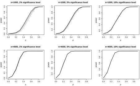
4.2.2 H1 rejection probability

The H1 rejection frequency of the LM, W, G and LR tests were calculated for several

values ofρ, i.e. ρ={0.1,0,2,0.3,0.4,0.5,0.6,0.7,0.8,0.9}, when ER was present. Rejection

frequency curves are presented in Figures 1 and 2 for the recursive and sample selection

model cases. All curves are nearly identical except for n = 1000 where the LM test seems

to have a marginal advantage. In all cases, theH1 rejection frequency improves as ρ and n

increase.

5

Applications

We illustrate the tests using two case studies in which the issue of endogeneity arises. The

first concerns a study, conducted in USA, on the impact of private health insurance on

0.0 0.2 0.4 0.6 0.8 0.0 0.2 0.4 0.6 0.8 1.0

n=1000, 1% significance level

ρ

po

w

er

0.0 0.2 0.4 0.6 0.8

0.2

0.4

0.6

0.8

1.0

n=1000, 5% significance level

ρ

po

w

er

0.0 0.2 0.4 0.6 0.8

0.2

0.4

0.6

0.8

1.0

n=1000, 10% significance level

ρ

po

w

er

0.0 0.2 0.4 0.6 0.8

0.0 0.2 0.4 0.6 0.8 1.0

n=4000, 1% significance level

ρ

po

w

er

0.0 0.2 0.4 0.6 0.8

0.2

0.4

0.6

0.8

1.0

n=4000, 5% significance level

ρ

po

w

er

0.0 0.2 0.4 0.6 0.8

0.2

0.4

0.6

0.8

1.0

n=4000, 10% significance level

ρ

po

w

[image:15.595.65.522.75.361.2]

er

Figure 1: Rejection frequency curves for theLM _{(solid curve),}W _(dotted), G_{(dotdashed) and}LR

(long-dashed) tests. The results refer to the recursive model case when ER is present. Note that in almost all cases the curves differ only minimally, hence they can hardly be distinguished.

0.0 0.2 0.4 0.6 0.8

0.0 0.2 0.4 0.6 0.8 1.0

n=1000, 1% significance level

ρ

po

w

er

0.0 0.2 0.4 0.6 0.8

0.2

0.4

0.6

0.8

1.0

n=1000, 5% significance level

ρ

po

w

er

0.0 0.2 0.4 0.6 0.8

0.2

0.4

0.6

0.8

1.0

n=1000, 10% significance level

ρ

po

w

er

0.0 0.2 0.4 0.6 0.8

0.0 0.2 0.4 0.6 0.8 1.0

n=4000, 1% significance level

ρ

po

w

er

0.0 0.2 0.4 0.6 0.8

0.2

0.4

0.6

0.8

1.0

n=4000, 5% significance level

ρ

po

w

er

0.0 0.2 0.4 0.6 0.8

0.2

0.4

0.6

0.8

1.0

n=4000, 10% significance level

ρ

po

w

er

Figure 2: Rejection frequency curves for theLM _{(solid curve),}W _(dotted), G_{(dotdashed) and}LR

[image:15.595.66.518.445.724.2]

http://www.meps.ahrq.gov/) which provides a sample that includes information on

de-mographics, individual health status, health care utilization and private health insurance

coverage. Private health insurance status is equal to 1 if the individual had a private health

insurance and 0 otherwise, and health care utilization is equal to 1 if the individual had at

least one visit to hospital outpatient departments. As suggested by many scholars,

estima-tion of such an effect can be biased by the possible endogeneity arising because unobserved

confounders (e.g., allergy and risk aversiveness) are likely to influence both health service

utilization and private insurance decision; full details can be found in Radice et al. (2015)

and references therein. The second dataset concerns the 2007 Zambian Demographic and

Health Survey (DHS; http://www.dhsprogram.com/) and the aim is to estimate the HIV

prevalence for men. HIV status (1 = positive, 0 = negative) and consent to test (1 =

consent, 0 = no consent) are recorded. Traditional methods assume that there are no

un-observed confounders associated with both HIV status and consent to test (Perez et al.,

2006). This assumption is unlikely to hold since a person’s belief about his or her HIV

status may be related to the actual status and hence influence the likelihood of consenting

to a test through unobservables. For instance, individuals who already know or suspect

that they are HIV positive may be less likely to consent. If this is the case then there will

be a selection bias in population prevalence estimates based on an incorrect assumption of

exogeneity (e.g., B¨arnighausen et al., 2011).

5.1

Analysis of health care utilization data

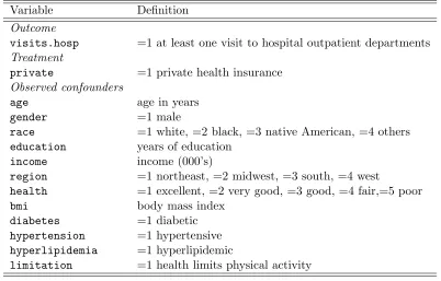
Following previous work on the subject (e.g., Radice et al., 2015, and references therein),

we specified a regression spline recursive bivariate probit model with main terms only. The

description of the variables used in the model are reported in Table 3. Specifically, the linear

predictors of the treatment (private) and outcome (visits.hosp) equations are

treat.eq <- private ~ as.factor(health) + as.factor(race) + as.factor(region)

+ limitation + gender + diabetes + hypertension

+ hyperlipidemia + self + s(bmi) + s(income) + s(age)

Variable Definition Outcome

visits.hosp =1 at least one visit to hospital outpatient departments Treatment

private =1 private health insurance Observed confounders

age age in years

gender =1 male

race =1 white, =2 black, =3 native American, =4 others

education years of education

income income (000’s)

region =1 northeast, =2 midwest, =3 south, =4 west

health =1 excellent, =2 very good, =3 good, =4 fair,=5 poor

bmi body mass index

diabetes =1 diabetic

hypertension =1 hypertensive

hyperlipidemia =1 hyperlipidemic

[image:17.595.96.498.65.322.2]

limitation =1 health limits physical activity

Table 3: Description of outcome and treatment variables, and observed confounders for MEPS data.

out.eq <- visits.hosp ~ private + as.factor(health) + as.factor(race)

+ as.factor(region) + limitation + gender + diabetes

+ hypertension + hyperlipidemia + self + s(bmi) + s(income)

+ s(age) + s(education)

where the smooth functions were represented using penalized thin plate regression splines

with basis dimensions equal to 20 and penalties based on second order derivatives (Wood,

2006). The non-linear specification for bmi, income, age and education arises from the

fact that these covariate embody productivity and life-cycle effects that are likely to

af-fect _P(private = 1) and _P(visits.hosp = 1) non-linearly. In fact, in related studies,

Holly et al. (1998) considered a model for health care utilization that contains linear and

quadratic terms in bmi, income, age and education, whereas Marra & Radice (2011b)

specified a model containing smooth functions of them. Note that for this case study it was

not possible to identify a suitable ER.

The effect of private onvisits.hosp (expressed in terms of average treatment effect

(ATE)) may be biased by the possible presence of unobserved confounding. We employed

were 0.005, 0.004 ,0.243 and 0.001 respectively. Because in simulation, LR andLM showed

reasonable empirical properties in the absence of ER, based on these tests’ results we can

assume that there is an issue of endogeneity. For completeness, we report the ATE (and

confidence interval) obtained when fitting the regression spline recursive bivariate probit

and the regression spline univariate probit for the outcome equation (i.e., the model not

accounting for endogeneity): 5.34% (3.85%,6.83%) and 4.29% (2.98%,5.60%), respectively.

The magnitude of the ATE found when accounting for endogeneity is higher, although the

confidence intervals overlap. In this case study the direction of the bias appears to be

downward. This result is counter-intuitive at first. If we assume that possible confounders

are allergy and risk aversiveness, then an upward bias should be expected (individuals with

a greater demand for medical care, say for reasons of poor health, are expected to have

a greater demand for insurance). The explanation behind this apparent contradiction is

that employer-provided insurance is generally limited to full-time workers and is positively

related to worker income. The empirical evidence indicates that workers who are in poorer

health are less likely to obtain employer-sponsored coverage (Buchmueller et al., 2005).

5.2

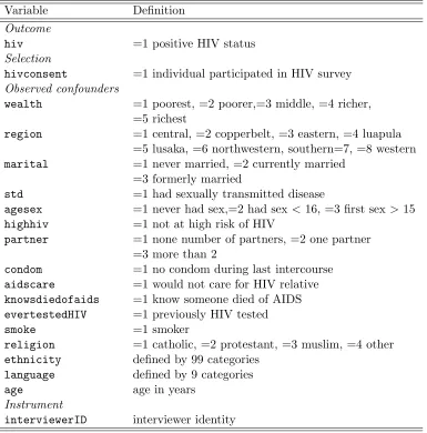
Analysis of HIV data

For the HIV dataset, using the variables in Table 4 and in line with the work by B¨arnighausen et al.

(2011), we specified the equations of the regression spline sample selection probit model as

sel.eq <- hivconsent ~ education + as.factor(wealth) + as.factor(region)

+ as.factor(marital) + std + as.factor(agesex) + highhiv

+ as.factor(partner) + condom + aidscare + knowsdiedofaids

+ evertestedHIV + smoke + as.factor(religion)

+ as.factor(ethnicity) + as.factor(language) + s(age)

+ as.factor(interviewerID)

out.eq <- hiv ~ education + as.factor(wealth) + as.factor(region)

+ as.factor(marital) + std + as.factor(agesex) + highhiv

+ evertestedHIV + smoke + as.factor(religion)

+ as.factor(ethnicity) + as.factor(language) + s(age)

Variable age is expected to have a non-linear impact on hiv as well as hivconsent,

whereaseducationwas included as a parametric component because it did not have enough

unique covariate values to justify the use of a smooth function. The selection equation

(hivconsent) also included interviewerID which served as ER. This was because,

ac-cording to B¨arnighausen et al. (2011) some interviewers are better than others at eliciting

consent to HIV testing. For example, respect for the elderly is high in Zambia and

peo-ple may find it more difficult to refuse testing from older interviewers than from younger

ones. In addition, interviewers’ personality traits, such as agreeableness or extraversion,

may affect the respondents’ likelihood of consenting to test.

The p-values obtained using the LM, W, G and LR tests were < 0.000, <0.000, 0.025

and 0.003. In the presence of ER, the simulation results showed that all tests perform well.

In this case study, the hypothesis of absence of endogenous sampling is rejected by all tests,

hence indicating that non-random selection should be accounted for when estimating the

HIV prevalence for men in Zambia. The HIV prevalence (and confidence interval) obtained

using the regression spline sample selection bivariate probit was 21% (20%,22%), which is

significantly higher as compared to 12% (11%,13%) calculated using the individuals who

consented to test.

6

Discussion

Observational studies are likely to be affected by the presence of unobserved confounders,

which may lead to inconsistent parameter estimates if not accounted for. For the case

of binary responses, the regression spline recursive and sample selection bivariate probit

models can be employed to deal with this problem. We discussed the likelihood ratio and

gradient tests within this class of models and compared their empirical performance with

that of the Lagrange multiplier and Wald tests through a Monte Carlo simulation study. The

results obtained allowed us to derive some guidelines which may be important for empirical

Variable Definition Outcome

hiv =1 positive HIV status

Selection

hivconsent =1 individual participated in HIV survey Observed confounders

wealth =1 poorest, =2 poorer,=3 middle, =4 richer, =5 richest

region =1 central, =2 copperbelt, =3 eastern, =4 luapula

=5 lusaka, =6 northwestern, southern=7, =8 western

marital =1 never married, =2 currently married =3 formerly married

std =1 had sexually transmitted disease

agesex =1 never had sex,=2 had sex <_{16, =3 first sex}> ₁₅

highhiv =1 not at high risk of HIV

partner =1 none number of partners, =2 one partner =3 more than 2

condom =1 no condom during last intercourse aidscare =1 would not care for HIV relative

knowsdiedofaids =1 know someone died of AIDS

evertestedHIV =1 previously HIV tested

smoke =1 smoker

religion =1 catholic, =2 protestant, =3 muslim, =4 other

ethnicity defined by 99 categories language defined by 9 categories

age age in years

Instrument

[image:20.595.107.492.204.594.2]

interviewerID interviewer identity

• when an exclusion restriction is present and under correct distributional specification,

all tests perform well;

• when it is not possible to impose an exclusion restriction and under correct

distribu-tional specification, the tests which showed a reasonable performance are the likelihood

ratio and Lagrange multiplier tests. This finding is of some interest as, in applied

stud-ies, identification of a valid instrument is not completely obvious and sometimes not

possible;

• when the assumption of correct distributional specification does not hold and an

ex-clusion restriction is present, the performance of all tests is worse than that observed

under correct specification. Nevertheless, the likelihood ratio and Lagrange multiplier

tests perform better relatively to the others;

• under the most challenging scenario (distributional misspecification and absence of

exclusion restriction), all tests do not exhibit a satisfactory performance although the

likelihood ratio and Lagrange multiplier tests seem to have a slight advantage over

the others.

Because the performance of the tests worsens when the assumption of normality does

not hold, tests based on different distributional assumptions may be considered. In the

HIV example, respondents with a strong negative score on the test variable have a high risk

of being HIV positive. This means that we would expect the presence of a non-Gaussian

dependence that a linear measure of association, such as the correlation coefficient, would

not be able to fully capture. In this direction, Radice et al. (2015) proposed regression

spline bivariate probit models which allow for non-linear dependencies between the outcome

equation and treatment or selection equation. This is achieved using Archimedean copula

functions as well as their rotated versions. Future research will look into the feasibility of

Acknowledgements

We thank the Editor and reviewer for their constructive criticism which helped to improve

the presentation of the article considerably.

Appendix: Further simulation details

InR, the equations for the recursive bivariate probit model were

eq1 <- y1 ~ m1 + s(z1) + s(z2)

eq2 <- y2 ~ y1 + m1 + s(z1)

where thes()indicate the unknown smooth functions described in Section 2, while y1, y2,

m1,z1 and z2 refer to y1i, y2i, m1i, z1i and z2i in Section 4. In the sample selection case, the

outcome equation was given as

eq2 <- y2 ~ m1 + s(z1)

For the case in whichz2_i did not enter the first equation of the DGP the equation was

eq1 <- y1 ~ m1 + s(z1)

P-values for the LM test were obtained using LM.bpm() from SemiParBIVProbit, that is

LM.bpm(list(eq1, eq2), data = dataSim, Model = ES),

where dataSimrepresents the data frame containing the variables associated with the two

equations simulated as explained in the previous section, and ES was set to "B" or "BSS"

depending on whether a recursive or sample selection bivariate probit model was considered.

The simultaneous bivariate model which was needed in order to calculate the p-values for

the other tests was fitted using

out <- SemiParBIVProbit(list(eq1, eq2), data = dataSim, Model = ES)

athr2 <- coef(out)["theta.star"]^2

v <- out$Vb

v.athr <- v[dim(v)[2], dim(v)[2]]

W <- athr2/v.athr

pchisq(W, 1, lower.tail = FALSE)

where athr2 and v.athr denote the estimates of ρ_∗ and Var(ρ_∗). P-values for the G test were obtained usinggt.bpm() fromSemiParBIVProbit, specifically gt.bpm(out). Finally,

p-values forLR in the recursive model case were obtained as follows

df11 <- round(out$edf1[1]) + 1

df12 <- round(out$edf1[2]) + 1

df21 <- round(out$edf2[1]) + 1

eq1FP <- y1 ~ m1 + s(z1, fx = TRUE, k = df11) + s(z2, fx = TRUE, k = df12)

eq2FP <- y2 ~ y1 + m1 + s(z1, fx = TRUE, k = df21)

outFP <- SemiParBIVProbit(list(eq1FP, eq2FP), fp = TRUE, data = dataSim, Model = ES)

log.sep <- logLik(outFP$gam1) + logLik(outFP$gam2)

log.sim <- logLik(outFP)

LR <- as.numeric(2*(log.sim-log.sep))

pchisq(LR, 1, lower.tail = FALSE)

where theedfare the estimated degrees of freedom of the smooth functions, and thedfrefer

to the number of basis functions used for each smooth term when fitting the unpenalized

bivariate probit model with splines (here achieved settingfx = TRUEandfp = TRUE).gam1

and gam2 refer to the fitted regression spline univariate probit models for the two model

equations; these were obtained usingmgcv. Because of identifiability constraints, one basis

function (specifically, the constant flat basis function) is always dropped from each smooth

term (Wood, 2006). Thus, each df needs to be increased by 1 to use the desired number

of degrees of freedom. If round(edf) is equal to 1 then there is no need to use a smooth

function and s() can be dropped from the variable involved. Of course, the expressions

for eq1FP and eq2FP varied based on the DGP and model (recursive or sample selection)

chosen using the univariate fits from gam1 and gam2. This did not lead to different results

as, in the majority of the replicates, the numbers of basis functions selected for the smooth

terms in the models were the same as those determined using the approach described above.

The smooth functions were represented using penalized thin plate regression splines with

basis dimensions equal to 20 and penalties based on second-order derivatives (Wood, 2006,

pp. 154–160). For theLR test, the basis dimension for each smooth function was equal to

df+ 1 and unpenalized thin plate regression splines were used.

References

Banasik, J. & Crook, J. (2007). Reject inference, augmentation, and sample selection.

European Journal of Operational Research, 183, 1582–1594.

B¨arnighausen, T., Bor, J., Wandira-Kazibwe, S., & Canning, D. (2011). Correcting HIV

prevalence estimates for survey nonparticipation using heckman-type selection models.

Epidemiology, 22, 27–35.

Buchmueller, T. C., Grumbach, K., Kronick, R., & Kahn, J. G. (2005). Book review:

The effect of health insurance on medical care utilization and implications for insurance

expansion: A review of the literature. Medical Care Research and Review, 62, 3–30.

Chib, S. & Greenberg, E. (2007). Semiparametric modeling and estimation of instrumental

variable models. Journal of Computational and Graphical Statistics, 16, 86–114.

Cuddeback, G., Wilson, E., Orme, J., & Combs-Orme, T. (2004). Detecting and statistically

correcting sample selection bias. Journal of Social Service Research, 30, 19–33.

de Ven, W. V. & Praag, B. V. (1981). The demand for deductibles in private health

insurance: a probit model with sample selection. Journal of Econometrics, 17, 229–252.

Eilers, P. H. C. & Marx, B. D. (1996). Flexible smoothing with B-splines and penalties.

Goldman, D., Bhattacharya, J., McCaffrey, D., Duan, N., Leibowitz, A., Joyce, G., &

Morton, S. (2001). Effect of insurance on mortality in an HIV-positive population in

care. Journal of the American Statistical Association, 96, 883–894.

Greene, W. H. (2012). Econometric Analysis. Prentice Hall, New York.

Han, S. & Vytlacil, E. J. (2014). Identification in a

gener-alization of bivariate probit models with endogenous regressors.

http://econ.sites.olt.ubc.ca/files/2013/12/pdf_paper_seminar_sukjin_han.pdf.

Hastie, T. & Tibshirani, R. (1993). Varying-coefficient models. Journal of the Royal

Sta-tistical Society Series B, 55, 757–796.

Heckman, J. (1978). Dummy endogenous variables in a simultaneous equation system.

Econometrica, 46, 931–959.

Heckman, J. (1979). Sample selection bias as a specification error. Econometrica, 47, 153–

161.

Holly, A., Gardiol, L., Domenighetti, G., & Brigitte, B. (1998). An econometric model of

health care utilization and health insurance in switzerland. European Economic Review,

42(3-5), 513–522.

Kauermann, G. (2005). Penalized spline smoothing in multivariable survival models with

varying coefficients. Computational Statistics and Data Analysis, 49, 169–186.

Kawatkar, A. A. & Nichol, M. B. (2009). Estimation of causal effects of physical activity

on obesity by a recursive bivariate probit model. Value in Health, 12, A131–A132.

Latif, E. (2009). The impact of diabetes on employment in Canada. Health Economics, 18,

577–589.

Liu, H. & Tu, W. (2012). A semiparametric regression model for paired longitudinal

out-comes with application in childhood blood pressure development. Annals of Applied

Maddala, G. S. (1983). Limited Dependent and Qualitative Variables in Econometrics.

Cambridge University Press, Cambridge.

Marra, G. & Radice, R. (2010). Penalised regression splines: theory and application to

medical research. Statistical Methods in Medical Research, 19, 107–125.

Marra, G. & Radice, R. (2011a). Estimation of a semiparametric recursive bivariate probit

model in the presence of endogeneity. Canadian Journal of Statistics, 39, 259–279.

Marra, G. & Radice, R. (2011b). A flexible instrumental variable approach. Statistical

Modelling, 11, 581–603.

Marra, G. & Radice, R. (2013). A penalized likelihood estimation approach to

semipara-metric sample selection binary response modeling. Electronic Journal of Statistics, 7,

1432–1455.

Marra, G. & Radice, R. (2015). SemiParBIVProbit: Semiparametric Bivariate Probit

Mod-elling. R package version 3.2-13.2.

Marra, G., Radice, R., & Missiroli, S. (2014). Testing the hypothesis of absence of

unob-served confounding in semiparametric bivariate probit models. Computational Statistics,

29, 715–741.

Monfardini, C. & Radice, R. (2008). Testing exogeneity in the bivariate probit model: A

monte carlo study. Oxford Bulletin of Economics and Statistics, 70, 271–282.

Montmarquette, C., Mahseredjiana, S., & Houle, R. (2001). The determinants of university

dropouts: a bivariate probability model with sample selection. Economics of Education

Review, 20, 475–484.

Nummi, T., Pan, J., Siren, T., & Liu, K. (2011). Testing for cubic smoothing splines under

dependent data. Biometrics, 67, 871–875.

Perez, F., Zvandaziva, C., Engelsmann, B., & Dabis, F. (2006). Acceptability of routine

hiv testing (opt-out) in antenatal services in two rural districts of zimbabwe. Journal of

R Development Core Team (2015). R: A Language and Environment for Statistical

Com-puting. R Foundation for Statistical Computing, Vienna, Austria. ISBN 3-900051-07-0.

Radice, R., Marra, G., & Wojtys, M. (2015). Copula regression spline models for binary

outcomes.

Radice, R., Marra, G., & Zanin, L. (2013). On the effect of obesity on employment in the

presence of observed and unobserved confounding. Statistica Neerlandica, 67, 436–455.

Ruppert, D., Wand, M., & Carroll, R. (2003). Semiparametric Regression. Cambridge

University Press, New York.

Terrell, G. (2002). The gradient statistic. Computing Science and Statistics, 34, 206–215.

Vargas, T., Ferrari, S., & Lemonte, A. (2013). Gradient statistic: Higher-order asymptotics

and bartlett-type correction. World Bank Economic Review, 7, 43–61.

Wilde, J. (2000). Identification of multiple equation probit models with endogenous dummy

regressors. Economics Letters, 69, 309–312.

Wood, S. N. (2006). Generalized Additive Models: An Introduction With R. Chapman &