Wind field effect on the power generation and aerodynamic performance of offshore floating wind turbines

Wind field effect on the power generation and aerodynamic performance of

offshore floating wind turbines

Liang Li, Yuanchuan Liu, Zhiming Yuan*_{, Yan Gao} 3

Department of Naval Architecture, Ocean and Marine Engineering, University of Strathclyde, UK

4

Abstract

This study is aimed at investigating wind field effect on the power generation and the aerodynamic 6

performance of offshore floating wind turbines. For this purpose, three comparative wind fields are 7

generated: a uniform wind field, a steady wind field with wind shear, and a turbulent wind field. Aero-8

hydro-servo coupled analysis is performed in time-domain to estimate how a referenced 9

semisubmersible offshore floating wind turbine behaves in the three wind fields. The results reveal the 10

importance of wind shear and inflow turbulence to the performance of the floating wind turbine. Thrust 11

force and power generation become very unstable in the presence of inflow turbulence. Due to the 12

control strategy of the wind turbine, the power generation is also correlated with operational state and 13

turbulence frequency. Although wind shear has a tiny effect on the rotor performance, the local 14

aerodynamic load applied at a single blade experiences fluctuation with the presence of wind shear. It 15

is also shown that the ultimate structural and fatigue damage loads at blade root are augmented by 16

inflow turbulence and wind shear. 17

Keywords: wind field; inflow turbulence; wind shear; power generation; aerodynamic performance; 18

offshore floating wind turbine 19

1.

Introduction

20

Global demand for energy is expected to climb by up to 25% [1] by 2040 and the world is pursuing 21

economic and sustainable energy sources to keep up with this considerable demand growth. In such 22

circumstance, the utilization of offshore wind energy resources is stimulated, leading to the 23

development of offshore floating wind turbine. Statoil [2] proposed a Spar-buoy floating wind turbine, 24

namely the Hywind concept, which is the first full-scale floating wind turbine that has ever been built. 25

Principle Power installed a full-scale 2MW WindFloat prototype near the coast of Portugal [3]. Most 26

recently, Hywind Scotland, the world’s first floating wind farm, already starts to deliver electricity to 27

the grid [4]. In addition to the installation of full-scale floating wind turbines, a series of model test 28

researches have been performed in the meanwhile [5-7]. The noticeable feature of offshore floating 29

wind turbines compared with traditional land-based wind turbines is that the wind turbine is mounted 30

on a floating platform displaced in the waves with mooring system. Therefore, the floating wind turbine 31

is also subject to wave loads. Besides, the dynamics of mooring lines also have an influence on the 32

response of floating wind turbines. Consequently, the study of offshore floating wind turbine is a multi-33

disciplinary coupled analysis. Liu et al. [8] developed a CFD simulation tool for the fully coupled model 34

of floating wind turbines. The aero-hydro-mooring coupled response of an integrated floating wind 35

turbine was examined in [9, 10]. 36

So far, the uniform wind field is usually assumed in the studies of floating wind turbine to simplify 37

the aerodynamic modelling [8-12]. Nevertheless, the real wind field in the natural world is far more 38

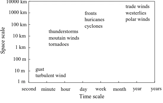
complex. Wind is by nature motion of air in the planetary boundary layer, and a stochastic process at 39

time and space scales [13] (see Fig. 1). The near-ground wind field is essentially gust or turbulent wind, 40

the modelling of which is usually based on classical assumptions on the probability density function of 41

wind speed and the shape of the wind profiles under various atmospheric stability conditions. That is to 42

say, the inflow turbulence and the wind shear are two basic features of a wind field. A couple of 43

approaches have been proposed, including the Kaimal and the Karman models, to model the inflow 44

turbulence. Most turbulence models are based on spectral method, which divides the turbulent inflow 45

into a set of turbulence components with various frequencies. In the space scale, the near-ground wind 46

field also varies with height. Popular models describing the wind profile include the power-law wind 47

profile, the low-level jet wind profile and the logarithmic wind profile. 48

49

Fig. 1. Classification of wind. 50

Apparently, the uniform wind field is deficient to evaluate the performance of offshore floating wind 51

turbines. In fact, previous measurements on land-based wind turbines have shown that the wind field 52

has an observable influence on the aerodynamic performance. Lubitz [14] investigated the ambient 53

turbulence on the energy production of a small wind turbine. It was concluded that turbulence was 54

beneficial to the power production at low wind speeds whereas reduced the power production at high 55

wind speeds. Li et al. [15] carried out model test in wind channel to study how the power generation of 56

a horizontal axis wind turbine reacted to the turbulent inflow. According to their measurement, the 57

optimum power coefficient was dependent on the turbulence intensity. Chamorro et al. [16] launched 58

an experiment to study the unsteady behaviour of a full-scale 2.5 MW wind turbine in turbulent inflow. 59

trade winds westerlies polar winds fronts

huricanes cyclones thunderstorms

moutain winds tornadoes 10000 km

1000 km 100 km 10 km

1 km 100 m 10 m 1 m

years year

month week day hour minute

Sp

ace

scal

e

Time scale second

gust

Their measurement also revealed a correlation between the turbulence intensity and the power 60

production. Similar relationship was observed by Lee et al. [17] in the field measurement of a small 61

vertical-axis wind turbine installed on the rooftop of a building. In addition to the inflow turbulence, 62

the realistic wind field also varies in vertical direction so that the wind shear effect should be considered 63

as well. Shen et al. [18] used the lifting surface method to simulate the unsteady and periodic blade root 64

loads and wind turbine performance in the presence of wind shear. Sezer-Uzol and Uzol [19] showed 65

that the existence of wind shear can create a very complex wake structure with substantial asymmetries, 66

streamwise vorticity generation, and non-periodicities downstream of the turbine rotor. Dolan and Lehn 67

[20] developed an analytical formulation for the torque of a three-bladed wind turbine with 68

consideration of the wind shear. They showed that the torque and the thrust force were only very slightly 69

influenced by the wind shear, but the local aerodynamic loads on a single blade were sensitive to the 70

wind shear. Similar phenomenon was observed by Li et al. [21]. 71

Although the effects of inflow turbulence and wind shear on the aerodynamic performance of wind 72

turbines have been manifested in previous studies, they were examined with a bottom-fixed wind 73

turbine, and no wind turbine active control was considered. In real practice, the floating platform 74

undertakes motions under joint aerodynamic and hydrodynamic excitations. Also, an offshore floating 75

wind turbine always incorporates a controller to regulate its power generation subject to various wind 76

speeds. For a floating wind turbine, the wind field effect may show new characteristics due to the aero-77

hydro-servo couplings. This study is aimed at investigating the effect of wind field on the performance 78

of offshore floating wind turbines, in terms of power generation, thrust force and blade root bending 79

moment. Aero-hydro-servo coupled analysis is conducted in time-domain to capture the performance 80

of a semisubmersible floating wind turbine in three categories of wind fields, namely a uniform wind 81

field, a steady wind field with consideration of wind shear and a turbulent wind field. The discussions 82

will be highlighted on how the performance of the floating wind turbine reacts to the wind shear and 83

the inflow turbulence. 84

2.

Model Description

85

As shown in Fig. 2, the OC4 DeepCwind semisubmersible concept [22] is considered in this work. 86

The wind turbine is the NREL 5 MW baseline wind turbine [23], which incorporates a variable-speed 87

torque controller and a blade pitch controller to regulate the power generation based on the operational 88

state. In below-rated state, the control strategy is to maximize the power generation by adjusting the 89

rotor speed. In over-rated state, the controller regulates the power generation by increasing the blade 90

92

Fig. 2. DeepCwind floating wind turbine system design [24]. 93

A three-column submersible platform is used to carry the wind turbine (see Fig. 3). The platform is 94

made up of three main offset columns inducing buoyance and restoring force, one central column 95

supporting the wind turbine, as well as a series of diagonal cross and horizontal bracing components. 96

To gain a good hydrostatic stability performance, a ballast tank is installed at the bottom of each main 97

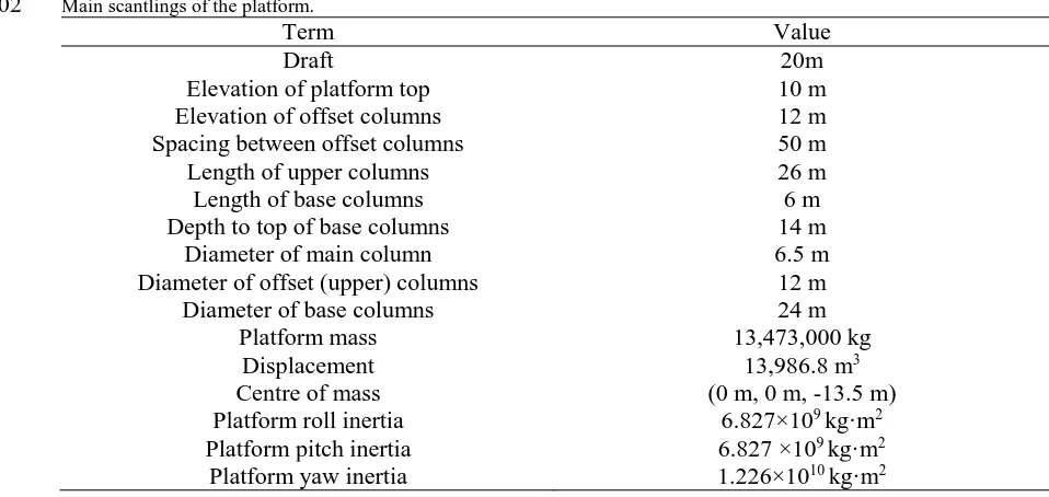
offset column. The main scantlings of the platform are listed in Table 1. 98

99

Table 1 101

Main scantlings of the platform. 102

Term Value

Draft 20m

Elevation of platform top 10 m

Elevation of offset columns 12 m

Spacing between offset columns 50 m

Length of upper columns 26 m

Length of base columns 6 m

Depth to top of base columns 14 m

Diameter of main column 6.5 m

Diameter of offset (upper) columns 12 m

Diameter of base columns 24 m

Platform mass 13,473,000 kg

Displacement 13,986.8 m3

Centre of mass (0 m, 0 m, -13.5 m)

Platform roll inertia 6.827×109 _kg·m2

Platform pitch inertia 6.827 ×109 _kg·m2

Platform yaw inertia 1.226×1010 _kg·m2

103

The floating wind turbine is displaced at sea site with a water depth of 200m. The mooring system 104

is composed of three catenary lines. The three mooring lines are oriented symmetrically at 60°, 180°, 105

and 300° about the vertical axis. Fairleads are connected to the tops of ballast tanks. The relevant 106

properties of mooring lines are outlined in Table 2. 107

Table 2 108

Properties of mooring line. 109

Term Value

Depth to anchor 200 m

Depth to fairlead 14 m

Radius to anchor 853.7 m

Radius to fairlead 40.868 m

Unstretched mooring line length 835.5 m

Mooring line diameter 0.0766 m

Equivalent line mass density 113.35 kg/m

Equivalent mooring line extensional stiffness 753.6 MN 110

3.

Methodology

111

The aero-hydro-servo coupled simulation code FAST [25] developed by the National Renewable 112

Energy Laboratory (NREL) is used to simulate the dynamic performance of the DeepCwind floating 113

wind turbine in various wind fields. 114

3.1.

Hydrodynamic modelling

115

The wave kinetics are addressed within the framework of potential flow theory, assuming that the 116

fluid is inviscous, incompressible and irrotational. Three components of hydrodynamic loads are 117

accounted: hydrostatic force, radiation wave force (including memory effect of the free water surface), 118

sufficiently long, second-order drift wave forces are also considered to capture the low-frequency 120

responses of the floating wind turbine. The hydrodynamic coefficients (added mass, potential damping, 121

wave force transfer function) are firstly calculated in frequency domain. By applying the Inverse FFT 122

(fast Fourier transform), the frequency-dependent coefficients are transformed to time-domain to 123

complete the simulations. 124

3.2.

Aerodynamic modelling

125

126

Fig. 4. Local inflow velocity at blade element. 127

Aerodynamic calculations are based on the blade element momentum (BEM) method, where the 128

blade is divided into a set of elements, and the elements are assumed independent from each other. The 129

distributed pressure and shear stress at each element are approximated by lift force and drag force. As 130

shown in Fig. 4, the BEM method calculates aerodynamic loads by evaluating the relative inflow speed 131

seen the by the blade element 132





1 (1 ')

1 tan

1 '

rel

r

u u a a

u

u a

r a

  





 

  _  _

 

 



 

 

(1) 133

where r is the radius of the blade element and Ω is the rotor speed. β is the blade pitch angle. a and a’

134

are the so-called axial and rotational induction factors, which are functions of attack angle θ and 135

aerodynamic coefficients of the blade. In practice, an initial condition of a and a’ is set, and the relative

136

speed is obtained. Afterwards, update a and a’ with the obtained relative speed. Iterate the process until

137

a and a’ converge, and the local aerodynamic loads are estimated by

138









2 2

2

1 (1 )

cos sin

2 sin

1 (1 ) (1 ')

sin cos

2 sin cos

l d

l d

u a

dT c C C dr

u a r a

dM c C C rdr

  



  

 



 

  

 

(2) 139

where ρ is the air density; c is the chord length; Cl and Cd are the lift coefficient and drag coefficient,

140

The iteration indicates that the relative velocity determined by the BEM method reacts 142

instantaneously to the change of incident inflow. In fact, the BEM method is a quasi-steady approach 143

and thereby it is usually applied in the steady problem, where the incident inflow is constant. For an 144

offshore floating wind turbine, both the platform motions and the wind turbulence produce unsteadiness 145

of the inflow seen by the rotor. The hysteresis effect caused by the unsteady inflow is accounted by the 146

extended Beddoes-Leishman (B-L) model developed by Minnema [26], which can be regarded as a 147

correction to the induced velocity determined by the BEM method. 148

3.3.

Wind turbine control

149

A variable-speed torque controller and a blade pitch controller are incorporated to the wind turbine. 150

The two control systems are designed to work independently, for the most part, in the below-rated

151

and above-rated wind-speed range, respectively. The goal of the variable-speed torque controller is to 152

maximize the power capture below the rated operation point. The goal of the blade-pitch controller is 153

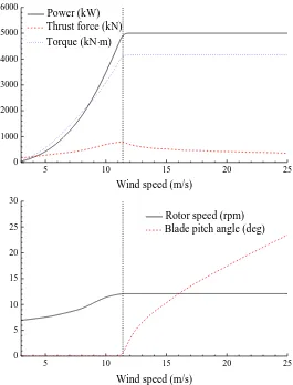
to regulate the generator power above the rated operation point. Fig. 5 illustrates the steady aerodynamic 154

performance of the NREL 5 MW baseline wind turbine under the regulation of the two controllers. 155

When the wind speed is lower than the rated value (11.4 m/s), the variable-speed torque controller is 156

active to tune rotor speed while the blade pitch is fixed at 0 deg to extract as much wind power as 157

possible. Within this range, the aerodynamic performance is quite sensitive to the wind speed, and the 158

power, the thrust force as well as the torque increase considerably with the wind speed. In over-rated 159

state, the blade pitch controller is active, and the rotor speed is fixed at 12.1 rpm. The blade is pitched 160

to feather to regulate the power generation. Meanwhile, the thrust force reduces as a result of the 161

163

Fig. 5. Steady aerodynamic performance of the wind turbine. 164

3.4.

Mooring system modelling

165

The lumped-mass model is used for the dynamics of mooring lines connected to the floating platform. 166

As shown in Fig. 6, the mooring line is divided into a set of evenly-sized segments, which are 167

represented by connected nodes and spring-damper systems. Each segment is divided into two 168

components and the properties are assigned and lumped to the two nodes at each end of that segment, 169

respectively. The connections between adjacent nodes are represented by damper-spring systems. Only 170

the axial properties of the mooring lines are accounted whereas the torsional and bending properties are 171

neglected. 172

173

Fig. 6. Lumped-mass model of mooring line. 174

5 10 15 20 25

0 1000 2000 3000 4000 5000 6000

Wind speed (m/s) Power (kW)

Thrust force (kN) Torque (kNm)

5 10 15 20 25

0 5 10 15 20 25 30

Wind speed (m/s)

Rotor speed (rpm) Blade pitch angle (deg)

Node 1

Node 2

Node 3

Segment 1

4.

Environmental conditions

In the natural world, the sea waves and offshore wind are always correlated. The joint wind-wave 176

model for the Statfjord site in the northern North Sea is used in this work [27]. Firstly, the mean wind 177

speed u at hub height (90 m above the mean sea level) is chosen. Subsequently, the fitting curve 178

provided in [27] is used to acquire the mean significant wave height Hs corresponding to a given mean

179

wind speed. Finally, the mean peak period Tp at given u and Hs is determined by Eq. (3). The

180

environmental conditions considered are listed in Table 3. The wind and waves propagate along positive 181

surge direction in all simulation cases. 182

0.78 0.529

0.78

(1.764 3.426 )

(4.883 2.68 ) 1 0.19

1.764 3.426 s

p s

s

u H

T H

H

     

    _ _{ }

 

 

  (3)

183

Table 3 184

Joint wind and waves conditions 185

u (m/s) Hs(m) Tp(s)

LC1 5.09 2.1 9.74

LC2 8.14 2.55 9.86

LC3 10.17 2.88 9.98

LC4 14.24 3.62 10.29

LC5 18.31 4.44 10.66

LC6 22.37 5.32 11.06

186

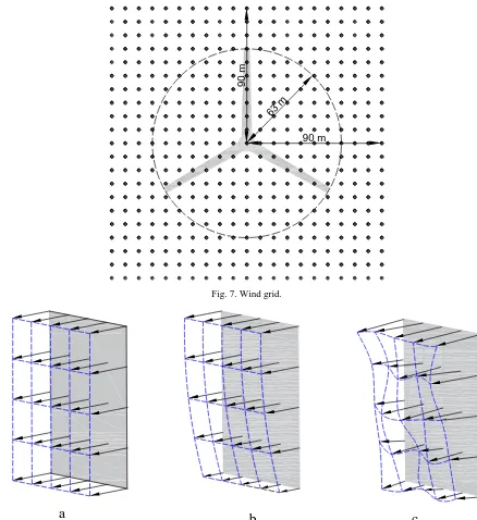
Given that the rotor diameter is 126 m, a wind grid with dimension 180 m × 180 m is generated (see 187

Fig. 7). Such configuration guarantees that the wind grid will cover the rotor all the time. 441 points 188

(21 × 21) are uniformly distributed across the area, at which the time-series of wind speed are generated. 189

As shown in Fig. 8, three comparative wind fields are generated for each load case, and the mean wind 190

192

Fig. 7. Wind grid. 193

194

Fig. 8. Three wind fields. (a) uniform wind field; (b) steady wind field with wind shear; (c) turbulent wind field. 195

The first wind field is uniform. The wind speed vector is constant, independent on spatial position 196

and time. It is the wind field that used in most studies of offshore floating wind turbine. 197

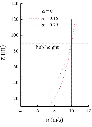
The second one is a steady wind field with consideration of wind shear, where the wind speed varies 198

only with height. The power-law model is used to represent the wind profile, 199

( )

90

z u z u



 

  

  (4)

200

where α is the exponent parameter. Fig. 9 shows the wind profiles with different values of α. The wind 201

shear becomes more significant when α increases. When α is equal to 0, the wind shear is omitted, and 202

the wind field reduces to the uniform one. In our study, α = 0.25 is used. 203

90 m

63 m

90 m

204

Fig. 9. Wind profile. 205

The first two wind fields are time-independent and the direction of inflow is always along X axis. In 206

the natural world, the wind speed not only varies in space scale but also depends on the time. Therefore, 207

a turbulent wind model should be adopted to describe this feature. The IEC Kaimal turbulent model [28] 208

is used to represent the turbulence in time scale. The time-series of wind speed are generated based on 209

the spectral method 210





2

5/3

4 /

( )

1 6 /

k k

k

k

L u S f

fL u





 (5)

211

where f is the cyclic frequency; k indicates the direction (longitudinal 1, lateral 2, vertical 3); Lk is

212

defined by Eq. (6) 213

8.10 1

2.70 2

0.66 3

k

k

L k

k

 

 

_  

 _{ }



(6) 214

where Λ is the turbulence scale parameter 215

0.7 min(60, hub height)

  (7)

216

σk is the standard deviation, which is defined by the turbulence intensity δ

217

1

2 1

3 1

100 0.8

0.5

u

 

 

 



 

(8) 218

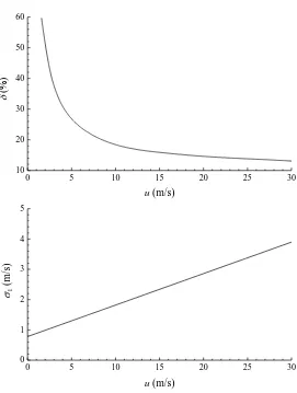
According to above equations, the spectrum of turbulent wind is totally dependent on the turbulence 219

intensity δ and the mean wind speed u. In the natural world, the turbulence intensity is correlated with 220

the mean wind speed, and the IEC category B turbulence model is used to determine the turbulence 221

intensity with respect to a given u. Fig. 10 shows the turbulence intensity and the corresponding standard 222

4 6 8 10 12

20 40 60 80 100 120 140

z (

m)

u (m/s)

 = 0

 = 0.15  = 0.25

deviation of longitudinal speed component at various mean wind speed. Although turbulent wind field 223

with high mean speed is has a small turbulence intensity, the standard deviation of wind speed is higher. 224

225

Fig. 10. Turbulence intensity and standard deviation of longitudinal wind speed as functions of mean wind speed. 226

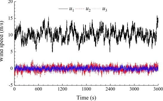
Fig. 11 displays the spectrum of turbulent wind and Fig. 12 plots the corresponding time-series of 227

wind speed. As shown, slow-varying component dominates the turbulent wind. Not only the amplitude 228

of the wind speed varies, but also the speed direction is time-dependent. 229

230

Fig. 11. Spectrum of IEC Kaimal turbulent wind, u = 10.17 m/s. 231

0 5 10 15 20 25 30

10 20 30 40 50 60





u (m/s)

0 5 10 15 20 25 30

0 1 2 3 4 5

1

(

m/s)

u (m/s)

0.0 0.1 0.2 0.3 0.4 0.5

0 20 40 60 80

S

(

(m

/s)

2 /H

z

2 )

f (Hz)

232

Fig. 12. Time-series of wind speed at height hub, u = 10.17 m/s. 233

Apart from the variation in time scale, the velocity of turbulent wind field is not uniformly 234

distributed across the rotor plane in a time instant, leading to the space scale turbulence. A spatial 235

coherence model is introduced to represent the phase difference of wind velocity at different spatial 236

points 237





, ,

2 2

,

( ) ( )

( ) ( )

( ) exp 12 0.12

min 60, hub height i j i j

i j

i j

c

c

S f Coh f

S f S f

fr r

Coh f

u L

L



 _{   } 

 

  _{    }

 _{   } 

 



(9) 238

where Si,j is the cross spectrum defining the correlation of the random wind speed at points i and j, r is

239

the distance between the two points. 240

5.

Results

241

The effects of wind shear and inflow turbulence on the performance of the DeepCwind floating wind 242

turbine will be investigated in this section, in terms of thrust force, power generation and blade root 243

bending moment. For all load cases, the simulation runs 4000 s and only the last 3600 s data are 244

collected to get rid of the transient effect arising in initial simulation stage. The time step is set to 0.0125 245

s. 246

5.1.

Thrust force

247

Fig. 13 illustrates the effect of wind shear on the rotor thrust force. It shows that the wind shear 248

effect is limited, which is consistent with previous studies [20, 21]. When a blade is experiencing the 249

high wind velocity region (up half of the rotor plane), the other two blades are within low wind velocity 250

region (down half of the rotor plane). Therefore, the resultant thrust force induced by the three blades 251

0 600 1200 1800 2400 3000 3600

-5 0 5 10 15 20

Wind

sp

eed (

m/s)

Time (s)

remains relatively stable. Of course, the aerodynamic load acting on each individual blade experiences 252

variation due to the wind shear, and this will be discussed in the following part of this paper. 253

254

Fig. 13. Thrust force with various wind shear. 255

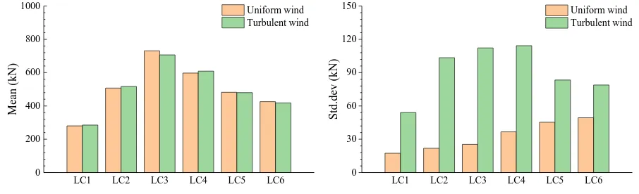
The statistics of thrust force in the turbulent wind field are showed in Fig. 14. Similarly, the average 256

thrust force is just slightly varied by the turbulence. Although the inflow is turbulent, the mean wind 257

speed is identical to that of the uniform wind field. Therefore, the mean thrust force acting on the rotor 258

is nearly the same. Nevertheless, the standard deviation is augmented significantly due to the inflow 259

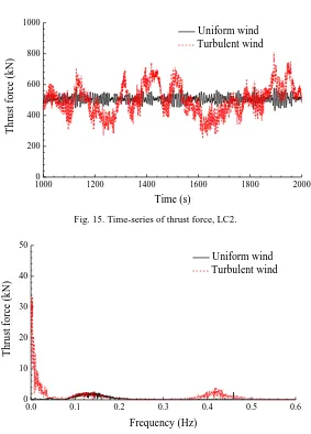
turbulence. Fig. 15 gives an example of the thrust force time history, where it can be seen that the thrust 260

force becomes very unstable in the presence of turbulence. Fig. 16 shows the FFT analysis result of 261

thrust force. Observable low-frequency response component is excited in the turbulent wind field. As 262

shown in Fig. 11, the turbulent wind is characterized by svarying component, and thereby the low-263

frequency component is mainly induced by the very slow variation of wind speed in time scale. 264

Additionally, the blades experience inflow velocity fluctuation during the rotation due to the space scale 265

turbulence, and thereby the thrust force is also excited at the 3P rotor frequency. The high-frequency 266

responses of wind turbines are relatively difficult to monitor, and various approaches have been 267

proposed. For example, Lind et al. [29] developed a normal behaviour model to monitor high-frequency 268

wind turbine vibrations. The excitation of high-frequency thrust force highlights the importance of wind 269

turbulence to the design of wind turbines. 270

271

Fig. 14. Thrust force with various turbulence intensity. 272

LC1 LC2 LC3 LC4 LC5 LC6

0 200 400 600 800 1000

Mean (kN)

Uniform wind Wind shear

LC1 LC2 LC3 LC4 LC5 LC6

0 20 40 60 80

Std

.dev (kN

)

Uniform wind Wind shear

LC1 LC2 LC3 LC4 LC5 LC6

0 200 400 600 800 1000

Mean (kN)

Uniform wind Turbulent wind

LC1 LC2 LC3 LC4 LC5 LC6

0 30 60 90 120 150

Std

.dev (kN

)

273

Fig. 15. Time-series of thrust force, LC2. 274

275

Fig. 16. FFT analysis result of thrust force, LC2. 276

The inflow turbulence influences not only the thrust force, but also the platform motions. 277

Considering that the surge natural period of the platform is sufficiently long (over 100 s [30]) and 278

covered by the dominating frequency range of the wind spectrum, resonant surge motion may be excited. 279

Fig. 17 represents the FFT analysis result of platform surge motion, where two response peaks are 280

observed. The first peak is located around 0.9 Hz, close to the wave energy frequency. This part of 281

motion is usually named as wave energy response, which is induced by first-order linear wave 282

excitations. Additionally, response is also observed around the natural period of surge motion, implying 283

that the resonant surge motion is excited by the second-order nonlinear wave drift forces. Due to the 284

slow-varying wind speed, the low frequency surge motion is amplified considerably by the inflow 285

turbulence. Nevertheless, the 3P rotor frequency response is not observed. It is mainly because the 3P 286

frequency is far from the resonant frequency of the platform so that the motions are not sensitive to the 287

space scale turbulence. 288

10000 1200 1400 1600 1800 2000

200 400 600 800 1000

Th

ru

st

f

o

rce (

k

N

)

Time (s)

Uniform wind Turbulent wind

0.0 0.1 0.2 0.3 0.4 0.5 0.6

0 10 20 30 40 50

Th

ru

st

f

o

rce (

k

N

)

Frequency (Hz)

289

Fig. 17. FFT analysis result of platform surge motion, LC2. 290

5.2.

Power generation

291

Fig. 18 represents the statistics of wind turbine power generation with respect to the three wind fields. 292

In general, the average power generation is merely dependent on the mean wind speed whereas varies 293

little with wind shear and inflow turbulence. The wind shear has a small influence on the fluctuation of 294

power generation. Nevertheless, the standard deviation increases significantly once the floating wind 295

turbine is subject to the turbulent inflow. According to Fig. 10, the standard deviation of wind speed 296

variation increases with the mean wind speed, so that the fluctuation of the power generation should 297

also be more noticeable. Such deduction is consistent with the variation trend in below-rated operational 298

state (LC1-LC3). Nevertheless, the fluctuation of power is reduced in over-rated operational sate (LC4-299

LC6), even if the wind field becomes more turbulent. It is attributed to the two controllers, which are 300

active in different operational states. In the below-rated state, the variable-speed torque controller is 301

active to maximise the power generation so that the power generation is very sensitive to the wind speed 302

(see Fig. 5). In this case, the power generation reacts promptly to the variation of wind speed and thereby 303

the standard deviation is augmented. Comparatively, it is the blade pitch controller that regulates the 304

wind turbine in the over-rated operational state, which aims to keep the power generation at the rated 305

value 5 MW. Consequently, the wind power remains relatively robust to the variation of wind speed. 306

Since the blade pitch controller is not perfect and takes time to react to the inflow, the fluctuation of 307

power generation is not omitted completely. 308

0.00 0.05 0.10 0.15 0.20 0.25 0.30

0.0 0.1 0.2 0.3 0.4 0.5 0.6

Su

rg

e (

m)

Frequency (Hz)

309

Fig. 18. Statistics of wind turbine power generation. 310

To figure out the dynamic feature of power generation, Fig. 19 demonstrates the FFT analysis result 311

of power generation when the wind turbine is operating in below-rated state, where three regions are 312

identified. This first region is located on the high frequency range where little response is observed. It 313

is mainly because the turbulent wind is slow-varying, and the turbulence spectrum carries little energy 314

around high frequency range (see Fig. 11). The power generation is most sensitive to the inflow 315

turbulence in the intermediate range of frequencies. Within this region, the power generation increases 316

rapidly as the varying frequency of the turbulent inflow reduces. The last region is the very low 317

frequency range. In the very low frequency range, the power generation is not sensitive to the variation 318

frequency of the turbulence. Similar phenomenon was observed in the field measurement of a full-scale 319

2.5 MW land-based wind turbine [16]. 320

321

Fig. 19. FFT analysis result of power generation in turbulent wind, LC2. 322

Fig. 20 shows the spectral property of the power generation in over-rated operation state. Despite 323

that three regions are identified, Fig. 20 shows a noticeable discrepancy compared with Fig. 19: the 324

power generation reacts little to the very low frequency turbulence component. It indicates that the 325

slow-varying turbulence is unable to stimulate strong fluctuation of power generation in the over-rated 326

operational state. 327

LC1 LC2 LC3 LC4 LC5 LC6

0 1000 2000 3000 4000 5000 6000

Mean (kW)

Uniform wind Wind shear Turbulent wind

LC1 LC2 LC3 LC4 LC5 LC6

0 300 600 900 1200

Std

.dev (kW)

Uniform wind Wind shear Turbulent wind

10-4 ₁₀-3 ₁₀-2 ₁₀-1 ₁₀0

0 30 60 90 120 150 180

III II

Po

w

er

g

ener

at

io

n

(

k

W)

Frequency (Hz)

328

Fig. 20. FFT analysis result of power generation in turbulent wind, LC5. 329

According to Fig. 19 and Fig. 20, one can see that the power generation reacts to the very low 330

frequency turbulence in different ways depending on the operational state. To interpret the mechanism 331

behind, we run an extra simulation to examine the reaction of power generation to inflow with various 332

oscillation frequencies, where the wind turbine is bottom-fixed and the wind shear is omitted. The time-333

varying inflow speed is defined as 334

0

( ) sin(2 )

( ) 2 cos(2 )

u t u u ft

du t f u ft



 

  

   (10)

335

where u0 is the mean wind speed and ∆u is the speed fluctuation. Two frequencies f are selected from 336

the second and the third regions, namely f = 0.01 Hz and f = 0.001 Hz. Also, u0 = 8.14 m/s and u0 = 337

18.31 m/s are selected to represent below-rated and over-rated operational states, respectively. ∆u is set 338

to 2 m/s in all cases. 339

Fig. 21 illustrates how the wind turbine responds to the inflow turbulence at below-rated and over-340

rated states, respectively. In the over-rated state, the power generation is nearly constant in the presence 341

of very slow-varying inflow whereas the power fluctuation is noticeable when the frequency is 342

sufficiently high. According to Eq. (10), the speed increment du of very low frequency turbulence 343

component is very small. The blade pitch controller is able to compensate the tiny external disturbance 344

and regulates the power generation. Consequently, the power generation reacts little to the very low 345

frequency turbulence component and keeps at the rated value 5MW. When f increases, the speed 346

increment is augmented accordingly. The pitch controller can’t afford to compensate the amplified 347

disturbance, and unstable power generation occurs. It explains why the power production is robust to 348

the very low frequency turbulence whereas sensitive to the moderate low frequency turbulence in Fig. 349

20. In the below-rated, nevertheless, the control objective is to maximize the power so that any tiny 350

variation of inflow speed will change the power generation, regardless of the wind speed varying 351

frequency (see Fig. 21(b)). In summary, the effect of inflow turbulence on the power generation is 352

dependent on the operational state due to the control scheme of the wind turbine. 353

10-4 ₁₀-3 ₁₀-2 ₁₀-1 ₁₀0

0 20 40 60

III II I

Po

w

er

g

ener

at

io

n

(

k

W)

354

Fig. 21. Reaction of power generation of sinusoidal inflow. (a) over-rated state, u0 = 18.31 m/s. (b) below-rated state, u0 = 355

8.14 m/s. 356

5.3.

Blade root bending moment

357

The generator of a wind turbine is driven by the blade, and blade root is the connection point of 358

blade and generator shaft. Therefore, blade root is a critical structure point, in terms of ultimate load 359

and fatigue damage. 360

The ultimate blade root bending moment is estimated based on the mean up-crossing rate method. 361

The distribution of extreme value Mmax is assumed to follow 362

max 0 0

0

( ) exp ( , )

T

P M M  _ v M t dt _





363

where 𝑣+(𝑀0, 𝑡) is the up-crossing rate corresponding to level 𝑀0, which denotes the instantaneous 364

frequency of the positive slop crossings of the defined level. The mean up-crossing rate is given by 365

0 0

0 1

( ) ( , )

T

v M v M t dt T

 _ 



366

S-N method is used to evaluate the corresponding fatigue damage load. It is assumed that the damage 367

accumulates linearly with each of hysteresis cycles according to Miner’s Rule. In this case, the overall 368

damage load (DL) produced by all the cycles is given by 369

200 400 600 800 1000

2000 3000 4000 5000 6000 7000 8000

Po

w

er

g

ener

at

io

n

(

k

W)

Time (s)

f = 0.001 Hz

f = 0.01 Hz

200 400 600 800 1000

0 1000 2000 3000 4000 5000 6000

Po

w

er

g

ener

at

io

n

(

k

W)

Time (s)

f = 0.001 Hz

f = 0.01 Hz

a

 





m m i i STeq

n L DL

n

 

 



 

 



(13)

370

where nSTeq =feq∙T is the total equivalent fatigue counts, feq (1 Hz in this paper) is the fatigue load

371

frequency and T is the simulation time. ni is the cycle count and Li is the cycle's load range about a fixed

372

load-mean. m is the Wholer exponent. Considering the geometry of the tower and the blade, the B1 373

category of S-N curve suggested by [31] is selected and m is set to 4. It worth noting that other 374

alternative approaches are available to estimate the fatigue loads. For example, Lind et al. [32] proposed 375

a procedure to estimate the fatigue loads on wind turbines, based on stochastic differential equations. 376

Fig. 22 displays the estimated mean up-crossing rate of the blade root bending moment. Regardless 377

of the operational state, the mean up-crossing rate is significantly increased by the inflow turbulence. 378

For example, the ultimate bending moment hardly exceeds 7000 kN∙m in the uniform wind field. On 379

the contrary, the mean up-crossing rate is as high as 10 Hz when the wind turbine is subject to turbulent 380

wind. Obviously, the bending moment is unstable in the turbulent wind field so that it has a higher 381

probability to exceed a certain level. 382

383

Fig. 22. Mean up-crossing rate of blade root bending moment, (a) LC2; (b) LC5. 384

Fig. 23 shows the fatigue damage load applied at the blade root. It is evident that the fatigue damage 385

bending moment increases with the inflow turbulence. In general, the fatigue damage bending moment 386

is doubled in the turbulent wind field. This is because the relative wind velocity seen by the blade 387

becomes very unstable in the presence of turbulence, and the fluctuation of blade root bending moment 388

is thus amplified. The result is that the load range of hysteresis cycle Li increases, augmenting the fatigue

389

damage load. 390

6000 7000 8000 9000 10000 11000 12000

10-4

10-3

10-2

10-1

100

M

ean u

p

-cr

o

ssing

r

at

e (

H

z)

M₀ (kNm)

Uniform wind Turbulent wind

5000 6000 7000 8000 9000 10000

10-4

10-3

10-2

10-1

100

M

ean u

p

-cr

o

ssing

r

at

e (

H

z)

M₀ (kNm)

Uniform wind Turbulent wind

391

Fig. 23. Fatigue damage bending moment at blade root. 392

Although the wind shear has little influence on the thrust force and the power generation, the blade 393

root bending moment is sensitive to wind shear. As shown in Fig. 24, the blade root bending moment 394

of an individual blade experiences increased fluctuation in the presence of wind shear. According to 395

the time-series, the dominating oscillating frequency of the bending moment is approximately 0.2 Hz, 396

close to the rotor speed. Apparently, this frequency is induced by both wind shear and tower shadow 397

effect. Given that the fluctuation of bending moment is amplified, the mean up-crossing rate and fatigue 398

load can be expected to increase accordingly. Fig. 25 and Fig. 26 supports this assumption. Due to the 399

increased fluctuation, the ultimate blade root bending moment has a higher probability to exceeds a 400

given level and the fatigue damage load accumulates more rapidly. 401

402

Fig. 24. Time series of blade root bending moment, LC3. 403

LC1 LC2 LC3 LC4 LC5 LC6

0 500 1000 1500 2000 2500 3000

D

L

(kN



m)

Uniform wind Turbulent wind

1000 1020 1040 1060 1080 1100

6000 8000 10000 12000

Be

n

d

in

g

mo

ment

(kN



m

)

Time (s)

404

Fig. 25. Mean up-crossing rate of blade root bending moment, (a) LC2; (b) LC5. 405

406

Fig. 26. Fatigue damage bending moment at blade root. 407

Although the overall performance of the wind turbine is just sensitive to inflow turbulence, the local 408

aerodynamic load at a single blade is nevertheless dependent on the wind shear. As well known, the 409

blade is one of the critical components of a wind turbine, which dominate the life time. Therefore, the 410

property of the local wind field must be carefully investigated. 411

6.

Conclusions

412

The effects of wind shear and inflow turbulence on the performance of a semisubmersible offshore 413

floating wind turbine are investigated in this work. A uniform wind field, a steady wind field with wind 414

shear and a turbulent wind field are generated. Aero-hydro-servo-elastic coupled analysis is performed 415

in time-domain to simulate the thrust force, the power generation and the blade root bending moment. 416

The wind shear has a limited influence on the rotor performance. Power generation and thrust force 417

are just slightly varied in the presence of wind shear. Nevertheless, the wind shear has a noticeable 418

effect on the local load applied at an individual blade. 419

Wind turbulence has a noticeable influence on the thrust force and the power generation. The 420

fluctuations of the two items are augmented when the wind turbine is subject to turbulent wind. Analysis 421

show that the reaction of power generation to very low frequency turbulence is dependent on the 422

operational state, due to the control strategy of the wind turbine. The power generation is insensitive to 423

6000 6200 6400 6600 6800 7000

10-5

10-4

10-3

10-2

10-1

100

M

ean u

p

-cr

so

ssing

r

at

e (

H

z)

M₀ (kNm)

Uniform wind Wind shear

5000 5500 6000 6500 7000 7500 8000

10-5

10-4

10-3

10-2

10-1

100

M

ean u

p

-cr

so

ssing

r

at

e (

H

z)

M₀ (kNm)

Uniform wind Wind shear

a b

LC1 LC2 LC3 LC4 LC5 LC6

0 500 1000 1500 2000 2500 3000

D

L

(kN



m)

very low frequency in the over-rated state whereas sensitive to any frequency turbulence in the below-424

rated state. 425

The ultimate and fatigue bending moment at the blade root is also examined. Both the ultimate and 426

fatigue damage loads increase as a result of inflow turbulence and wind shear. 427

This study reveals that a uniform wind field is far from sufficient for the estimation of floating wind 428

turbine behaviour. The wind shear and inflow turbulence must be taken into account to avoid premature 429

failure. 430

Acknowledgement

The authors would like to acknowledge China Scholarship Council for the financial support (No. 432

201506230127). 433

References

[1] ExxonMobile. Outlook for Energy: A View to 2040. 2018; 10. 435

[2] Nielsen FG, Hanson TD, Skaare B. Integrated dynamic analysis of floating offshore wind turbines. 436

Proceedings of the 25th Internatioanl Conference on Offshore Mechanics and Artic Engineering, 437

Humburg. 2006; 1:671-679. http://doi.org/10.1115/OMAE2006-92291. 438

[3] Principle Power. WindFloat, 439

http://www.principlepowerinc.com/en/windfloat/; 2015 440

[accessed 27 March 2018] 441

[4] Statoil. World’s first floating wind farm has started production, 442

https://www.statoil.com/en/news/worlds-first-floating-wind-farm-started-production.html/; 2017. 443

[accessed 27 March 2018] 444

[5] Li L, Gao Y, Hu ZQ, Yuan ZM, Day S, Li HR. Model test research of a semisubmersible floating 445

wind turbine with an improved deficient thrust force correction approach. Renew Energ. 2018;119:95-446

105. http://doi.org/10.1016/j.renene.2017.12.019. 447

[6] Duan F, Hu Z, Wang J. Model Tests of a Spar-Type Floating Wind Turbine Under Wind/Wave 448

Loads. Proceedings of the 34th Internatioanl Conference on Offshore Mechanics and Artic Engineering, 449

St. John’s. 2015; 9: V009T09A044 . http://doi.org/10.1115/OMAE2015-41391. 450

[7] Goupee AJ, Koo BJ, Kimball RW, Lambrakos KF, Dagher HJ. Experimental Comparison of Three 451

Floating Wind Turbine Concepts. J Offshore Mech Arct Eng. 2014;136(2):020906. 452

http://doi.org/10.1115/1.4025804. 453

[8] Liu YC, Xiao Q, Incecik A, Peyrard C, Wan DC. Establishing a fully coupled CFD analysis tool for 454

floating offshore wind turbines. Renew Energ. 2017;112:280-301. https:// 455

[9] Li L, Gao Y, Yuan ZM, Day S, Hu ZQ. Dynamic response and power production of a floating 457

integrated wind, wave and tidal energy system. Renew Energ. 2018;116:412-22. https://doi.org/ 458

10.1016/j.renene.2017.09.080. 459

[10] Li L, Cheng Z, Yuan Z, Gao Y. Short-term extreme response and fatigue damage of an integrated 460

offshore renewable energy system. Renew Energ. 2018;126:617-29. https:// 461

doi.org/10.1016/j.renene.2018.03.087 462

[11] Li L, Hu ZQ, Wang J, Ma Y. Development and Validation of an Aero-hydro Simulation Code for 463

Offshore Floating Wind Turbine. J Ocean Wind Energy. 2015;2(1):1-11. 464

[12] Liu YC, Xiao Q, Incecik A, Wan DC. Investigation of the effects of platform motion on the 465

aerodynamics of a floating offshore wind turbine. J Hydrodyn. 2016;28(1):95-101. 466

https://doi.org/10.1016/S1001-6058(16)60611-X 467

[13] Orlanski I. A rational subdivision of scales for atmospheric processes. Bulletin of the American 468

Meteorological Society. 1975:527-30. 469

[14] Lubitz WD. Impact of ambient turbulence on performance of a small wind turbine. Renew Energ. 470

2014;61:69-73. https://doi.org/10.1016/j.renene.2012.08.015. 471

[15] Li QA, Murata J, Endo M, Maeda T, Kamada Y. Experimental and numerical investigation of the 472

effect of turbulent inflow on a Horizontal Axis Wind Turbine (Part I: Power performance). Energy. 473

2016;113:713-22. https://doi.org/10.1016/j.energy.2016.06.138 474

[16] Chamorro LP, Lee SJ, Olsen D, Milliren C, Marr J, Arndt REA, et al. Turbulence effects on a full-475

scale 2.5 MW horizontal-axis wind turbine under neutrally stratified conditions. Wind Energy. 476

2015;18(2):339-49. https://doi.org/10.1002/we.1700 477

[17] Lee KY, Tsao SH, Tzeng CW, Lin HJ. Influence of the vertical wind and wind direction on the 478

power output of a small vertical-axis wind turbine installed on the rooftop of a building. Appl Energ. 479

2018;209:383-91. https://doi.org/10.1016/j.apenergy.2017.08.185. 480

[18] Shen X, Zhu XC, Du ZH. Wind turbine aerodynamics and loads control in wind shear flow. Energy. 481

2011;36(3):1424-34. https://doi.org/10.1016/j.energy.2011.01.028 482

[19] Sezer-Uzol N, Uzol O. Effect of steady and transient wind shear on the wake structure and 483

performance of a horizontal axis wind turbine rotor. Wind Energy. 2013;16(1):1-17. 484

https://doi.org/10.1002/we.514 485

[20] Dolan DSL, Lehn PW. Simulation model of wind turbine 3p torque oscillations due to wind shear 486

and tower shadow. IEEE Tranc Energy Conver. 2006;21(3):717-24.

487

http://doi.org/10.1109/TEC.2006.874211. 488

[21] Li Y, Castro AM, Sinokrot T, Prescott W, Carrica PM. Coupled multi-body dynamics and CFD 489

for wind turbine simulation including explicit wind turbulence. Renew Energ. 2015;76:338-61. 490

[22] Robertson A, Jonkman J, Masciola M, Song H, Goupee A, Coulling A, et al. Definition of the 492

semisubmersible floating system for phase II of OC4. National Renewable Energy Laboratory (NREL), 493

Golden, CO.; 2014. 494

[23] Jonkman JM, Butterfield S, Musial W, Scott G. Definition of a 5-MW reference wind turbine for 495

offshore system development. National Renewable Energy Laboratory Golden, CO; 2009. 496

[24] Coulling AJ, Goupee AJ, Robertson AN, Jonkman JM, Dagher HJ. Validation of a FAST semi-497

submersible floating wind turbine numerical model with DeepCwind test data. Journal of Renewable 498

and Sustainable Energy. 2013;5(2):023116. https://doi.org/10.1063/1.4796197. 499

[25] Jonkman JM, Buhl Jr ML. FAST User's Guide. National Renewable Energy Laboratory (NREL); 500

2005. 501

[26] Minnema JE. Pitching moment predictions on wind turbine blades using the Beddoes-Leishman 502

model for unsteady aerodynamics and dynamic stall: Department of Mechanical Engineering, 503

University of Utah, 1998. 504

[27] Johannessen K, Meling TS, Hayer S. Joint distribution for wind and waves in the northern north 505

sea. Proceedings of 17th International Offshore and Polar Engineering Conference, Stavanger, 2001; 506

3:19-28. 507

[28] International Electrotechnical Commission. Standard: IEC 61400-1 Wind turbines part 1: Design 508

requirements. 2015. 509

[29] Lind PG, Vera-Tudela L, Wahter M, Kuhn M, Peinke J. Normal Behaviour Models for Wind 510

Turbine Vibrations: Comparison of Neural Networks and a Stochastic Approach. Energies. 511

2017;10(12):1944. https://doi.org/10.3390/en10121944. 512

[30] Li L, Hu Z, Wang J, Hu Q. Dynamic Responses of a Semi-type Offshore Floating Wind Turbine. 513

Proceedings of the 33rd Internatioanl Conference on Offshore Mechanics and Artic Engineering, San 514

Francisco. 2014; 9A: V09AT09A009. https://doi.org/10.1115/OMAE2014-23182. 515

[31] Det Norske Veritas. Fatigue design of offshore steel structures. Standard: DNV-RP-C203. 2010. 516

[32] Lind PG, Herraez I, Wachter M, Peinke J. Fatigue Load Estimation through a Simple Stochastic 517

Model. Energies. 2014;7(12):8279-93. https://doi.org/10.3390/en7128279. 518