dsmcFoam+ : an OpenFOAM based direct simulation Monte Carlo solver

Contents lists available atScienceDirect

Computer Physics Communications

journal homepage:www.elsevier.com/locate/cpc

Feature article

dsmcFoam+: An OpenFOAM based direct simulation Monte Carlo

solver

✩

C. White

a,

*

, M.K. Borg

b

, T.J. Scanlon

c

, S.M. Longshaw

d

, B. John

d

, D.R. Emerson

d

,

J.M. Reese

b

a_{School of Engineering, University of Glasgow, Glasgow G12 8QQ, UK} b_{School of Engineering, University of Edinburgh, Edinburgh EH9 3FB, UK}

c_{Department of Mechanical and Aerospace Engineering, University of Strathclyde, Glasgow G1 1XJ, UK}

d_{Scientific Computing Department, The Science & Technology Facilities Council, Daresbury Laboratory, Warrington, Cheshire WA4 4AD, UK}

a r t i c l e i n f o

Article history:

Received 6 March 2017

Received in revised form 21 August 2017 Accepted 25 September 2017

Available online 24 October 2017

Keywords:

dsmcFoam+ OpenFOAM

direct simulation Monte Carlo DSMC

Hypersonics Nano-scale Micro-scale Rarefied gas dynamics

a b s t r a c t

dsmcFoam+ is a direct simulation Monte Carlo (DSMC) solver for rarefied gas dynamics, implemented within the OpenFOAM software framework, and parallelised with MPI. It is open-source and released under the GNU General Public License in a publicly available software repository that includes detailed documentation and tutorial DSMC gas flow cases. This release of the code includes many features not found in standard dsmcFoam, such as molecular vibrational and electronic energy modes, chemical reactions, and subsonic pressure boundary conditions. Since dsmcFoam+ is designed entirely within OpenFOAM’s C++object-oriented framework, it benefits from a number of key features: the code empha-sises extensibility and flexibility so it is aimed first and foremost as a research tool for DSMC, allowing new models and test cases to be developed and tested rapidly. All DSMC cases are as straightforward as setting up any standard OpenFOAM case, as dsmcFoam+ relies upon the standard OpenFOAMdictionarybased directory structure. This ensures that useful pre- and post-processing capabilities provided by OpenFOAM remain available even though the fully Lagrangian nature of a DSMC simulation is not typical of most OpenFOAM applications. We show that dsmcFoam+ compares well to other well-known DSMC codes and to analytical solutions in terms of benchmark results.

Program summary

Program title:dsmcFoam+

Program Files doi:http://dx.doi.org/10.17632/7b4xkpx43b.1

Licensing provisions:GNU General Public License 3 (GPL)

Programming language:C++

Nature of problem:dsmcFoam+ has been developed to help investigate rarefied gas flow problems using the direct simulation Monte Carlo (DSMC) method. It provides an easily extended, parallelised, DSMC environment.

Solution method: dsmcFoam+ implements an explicit time-stepping solver with stochastic molecular collisions appropriate for studying rarefied gas flow problems.

References:All appropriate methodological references are contained in the section entitledReferences.

©2017 The Authors. Published by Elsevier B.V. This is an open access article under the CC BY license (http://creativecommons.org/licenses/by/4.0/).

1. Introduction

The direct simulation Monte Carlo (DSMC) technique is a stochastic particle-based method for simulating dilute gas flow problems. The method was pioneered by Bird [1] in the 1960s and has since become one of the most accepted methods for solving gas flows in the non-equilibrium Knudsen number regime. In a DSMC simulation, a single particle represents a large number of real gas atoms or molecules, reducing the computational expense relative to a fully deterministic method such as molecular dynamics (MD). Each of these particles is

✩_{This paper and its associated computer program are available via the Computer Physics Communication homepage on ScienceDirect (http://www.sciencedirect.com/} science/journal/00104655).

*

Corresponding author.

E-mail address:craig.white.2@glasgow.ac.uk(C. White).

https://doi.org/10.1016/j.cpc.2017.09.030

[image:2.595.122.485.73.193.2]

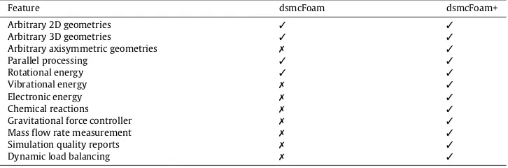
Table 1

Comparison of dsmcFoam and dsmcFoam+ capabilities.

Feature dsmcFoam dsmcFoam+

Arbitrary 2D geometries ✓ ✓

Arbitrary 3D geometries ✓ ✓

Arbitrary axisymmetric geometries ✗ ✓

Parallel processing ✓ ✓

Rotational energy ✓ ✓

Vibrational energy ✗ ✓

Electronic energy ✗ ✓

Chemical reactions ✗ ✓

Gravitational force controller ✗ ✓

Mass flow rate measurement ✗ ✓

Simulation quality reports ✗ ✓

Dynamic load balancing ✗ ✓

free to move in space, according to its own velocity and the local time step, and to interact with other particles and the boundaries of the system. Inter-particle collisions are handled in a stochastic manner after all particle movements have taken place. In this way, an evolving simulation emulates the physics of a real gas rather than attempting to solve Newton’s equations of motion for a very large number of individual atoms/molecules, as in MD.

The software application described in this article, dsmcFoam (later, dsmcFoam+), fulfils a similar role to alternatives such as MONACO [2], DAC [2], or SPARTA [3] (to name a few). However, it is distinct from these others because all of its functionality is built entirely within OpenFOAM [4]. This provides a built-in level of modularity, as well as potential interoperability by way of coupling with a large selection of other solver types that are also available in OpenFOAM. It is released open-source under the same General Public License (GPL) as the version of OpenFOAM it currently uses as its base. Up-to-date versions of dsmcFoam+, along with the OpenFOAM base it uses, are publicly available via a repository [5].

OpenFOAM [4] (or Open-sourceFieldOperationAndManipulation) is an open-source suite of libraries and applications initially designed to solve computational fluid dynamics (CFD) problems. It has become more complex over the years since its initial release, but its basic principle remains the same: to provide an open and extensible C++based software package containing a wide range of libraries, pre- and post-processing tools, and solvers, as well as a framework that can be used to build new applications.

dsmcFoam has been released with OpenFOAM since version 1.7. It was initially developed by OpenCFD Ltd, in collaboration with Scanlon et al. [6], as an extension to the molecular dynamics solvermdFoamdeveloped by Macpherson et al. [7–11]. The core DSMC functionality of dsmcFoam has since remained largely unchanged and can be found in the current release of OpenFOAM.

This article concerns a branch of dsmcFoam that has undergone significant development since the original was accepted into OpenFOAM, and is referred to henceforth as dsmcFoam+. The executable is named dsmcFoamPlus in order to conform with long-standing OpenFOAM naming conventions using only alphabetic characters. This solver is a direct continuation and development of the original dsmcFoam, branched following its release with OpenFOAM-1.7. It provides an enhanced set of DSMC capabilities when compared to dsmcFoam [12–18], as well as new capabilities in terms of parallel performance through the introduction of dynamic load balancing. Table 1gives an overview of the differences between dsmcFoam and dsmcFoam+. In addition to these key feature differences, dsmcFoam+ includes a greatly extended suite of boundary conditions and macroscopic property measurement tools compared to dsmcFoam.

In basing the core functionality of dsmcFoam+ around standard OpenFOAM libraries, the code is able to make use of powerful meshing facilities, parallelised Lagrangian/mesh-tracking algorithms, templated particle classes, and pre- and post-processing methods. As an example of this, DSMC particles are initially defined by linking their coordinates within cells of the mesh of a problem domain. As the application is built on top of this meshing capability, this also means that typical OpenFOAM pre- and post-processing applications can be used, such as domain-decomposition and reconstruction of the mesh for parallel processing based on cells (and hence the particles), as well as visualising results via ParaView [19]. Access to the mesh processing capabilities of OpenFOAM provides a powerful tool to define DSMC simulations with complex mesh structures, which are often a requirement for three-dimensional, realistic geometries.

A key strength of dsmcFoam+ comes from its strict adherence to OpenFOAM coding practices, meaning that its design is almost entirely modular in the form of C++classes. As an example, if it is desirable to add a new binary particle collision formulation then all that needs to be done is to create a copy of the existing derived binary collision classes (which are themselves specialisms of the base binary collision class) and then modify the algorithm that it implements in order to calculate the new routine. Once this new class is included in the application’s compilation, it automatically becomes available as a valid selection for a case. In order to use the new collision model, the user then only needs to change the textual description in the appropriate configuration file.

2. Direct simulation Monte Carlo with dsmcFoam+

2.1. Background

Rarefied gas dynamics is the study of gas flows in which the molecular mean free path,

λ

, is not negligible with respect to the characteristic length scale,L, of the system under consideration. The degree of rarefaction is defined by the Knudsen number,

Kn

=

λ

L

.

(1)

In the limit of zero Knudsen number, inter-molecular collisions dominate and the gas is in perfect thermodynamic equilibrium. But, as the Knudsen number increases, molecular collisions become less frequent until the free-molecular limit is reached where inter-molecular collisions are very unlikely. Since it is inter-molecular collisions and gas–surface interactions that drive a system towards thermodynamic equilibrium, it is clear that non-equilibrium effects become dominant with increasing Knudsen number. The different Knudsen number regimes are illustrated inFig. 1.

[image:3.595.137.450.51.120.2]

Fig. 1.Knudsen number regimes, adapted from Ref. [20].

•

Kn

→

0: inviscid flow (Euler fluid equations);

•

Kn

≤

0

.

001: continuum regime (Navier–Stokes–Fourier fluid equations);

•

0

.

001

≤

Kn

≤

0

.

1: slip regime (Navier–Stokes–Fourier fluid equations with velocity-slip and temperature-jump boundary conditions);

•

0

.

1

≤

Kn

≤

10: transition regime (Boltzmann equation or particle methods such as DSMC);

•

Kn

≥

10: free-molecular regime (collisionless Boltzmann equation or particle methods such as DSMC).

2.1.1. Continuum regime

For the continuum flow regime, the familiar Navier–Stokes–Fourier (NSF) continuum-fluid equations provide an excellent approxima-tion for gas flows that are very close to equilibrium. It is assumed that local macro-properties can be described as averages over elements that are large compared to the microscopic structure of the fluid, but small enough with respect to the macroscopic phenomena to permit the use of differential calculus. Inter-molecular collisions are dominant at low Knudsen number, i.e. there are enough molecular collisions occurring for local thermodynamic equilibrium to be reached in a very short time compared to the macroscopic time scale. In the limit of zero Knudsen number, the NSF equations can be reduced to the inviscid Euler equations because molecular diffusion can be ignored, and so the transport terms in the continuum momentum and energy equations are negligible [20].

2.1.2. Slip regime

As the Knudsen number becomes significant, molecule–surface interactions become less frequent and regions of non-equilibrium start to appear near surfaces. This can be observed from a macroscopic point of view as the gas velocity and temperature (Ug andTg) at a

surface not obtaining the same values as the surface itself (UsandTs). These phenomena are known as velocity-slip and temperature-jump,

respectively. If this type of non-equilibrium is in the flow, the range of validity of the NSF equations can be extended to the slip regime by applying Maxwell’s velocity-slip [21] and Von Smoluchowski’s temperature-jump [22] boundary conditions.

2.1.3. Transition and free-molecular regimes

In the transition and free-molecular regimes, non-equilibrium effects dominate and a solution to the Boltzmann equation must be sought, as the assumption of linear constitutive relations in the NSF equations is no longer valid. Examples include flows in micro-scale geometries (e.g. micro-channels) [23], and hypersonic flows, particularly at low ambient pressures [24]. In these cases, the Navier–Stokes– Fourier (NSF) equations fail to give accurate predictions of the flow behaviour because the assumptions of a continuum fluid and local equilibrium break down. Recourse to the Boltzmann equation must be sought for an accurate description of the flow behaviour. The Boltzmann equation for a single-species, monatomic, non-reacting gas takes the form:

∂ (

nf

)

∂

t

+

c

∂ (

nf

)

∂

r

+

F

∂ (

nf

)

∂

c

=

J

(

f

,

f∗

)

,

(2)

wherenf is the product of the number density and the normalised molecular velocity distribution function,randcare the position and velocity vectors of a molecule, respectively,Fis an external force,J

(

f

,

f∗

₎

is a non-linear integral that describes the binary collisions, and the superscript

∗

represent post-collision properties. The collision integral takes the form:

J

(

f

,

f∗

)

=

∫

∞

−∞

∫

4π

0

n2

(

f∗f₁∗

−

ff1

)

cr

σ

TdΩdc1

,

(3)

wherefandf1are the velocity distribution function atcandc1respectively,cris the relative speed of two colliding molecules,

σ

Tis the

molecular cross-section, andΩis the solid collision angle.

In 1992, a mathematical proof that the DSMC method provides a solution to the Boltzmann equation for a monatomic gas in the limiting case of an infinite number of particles was published [25], removing any remaining ambiguity over how DSMC relates to the Boltzmann equation. The DSMC method is comprehensively described in Bird’s 1994 and 2013 monographs [1,26].

2.2. Initialisation

A DSMC simulation performed using dsmcFoam+ begins with a set of pre-located particles. This process is achieved using pre-processing tools and involves specifying the positions of the domain extremities, the velocities of the particles, and the type of particles (i.e. species, mass, internal energy parameters). The user specifies macroscopic values of temperature, velocity, and density that are then used to insert particles with energies and positions that return, on average, these macroscopic parameters.

[image:4.595.217.384.59.377.2]

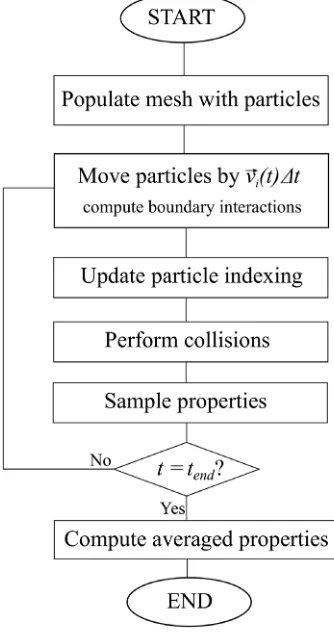
Fig. 2.Flow chart of the basic DSMC time-integration scheme.

2.3. Algorithmic overview

dsmcFoam+ implements an explicit time-stepping scheme in order to move particles in time and space within the computational domain. The basic algorithm that all DSMC solvers follow, including dsmcFoam+, can be described for a single DSMC time-step,t

→

t

+

∆t, as follows, and shown inFig. 2:

Step 1Update the position of allNparticles in the system using OpenFOAM’s inbuilt particle tracking algorithm [27], as discussed in Section2.4, which handles motion of particles across faces of the mesh (and also deals with boundaries). In its mathematical form, the move step for theith particle is given by:

⃗

ri

(

t

+

∆t

)

= ⃗

ri

(

t

)

+ ⃗

v

i

(

t

)

∆t

= ⃗

ri

(

t

)

+

∆

⃗

ri (4)

Step 2Update the list of particles in each computational cell to prepare for the collision routine.

Step 3Compute the number of collisions to attempt in each computational cell. The numerical implementation of this step is

described in Section2.5.

Step 4Perform the collisions according to the user-defined binary collision model.

Step 5Sample the particle positions, velocities, internal energies, etc. that are required to return the desired macroscopic values.

Step 6Go back toStep 1, where nowt

=

t

+

∆tand repeat again until the simulation end-timetendhas been reached.

2.4. Movement: Particle tracking

The particle tracking algorithm [27] on which dsmcFoam+ is based is an existing OpenFOAM functionality for the discrete motion of particles within a mesh, with the two important objectives of knowing when particles switch cells in the mesh and dealing with particles as they interact with boundaries. To facilitate this, a robust way of tracking particles within a mesh is required. Rather than applying∆

⃗

ri

2.5. Binary collisions

After all of the particles have moved and been tracked to their new positions in the mesh, it is necessary to re-index them before beginning the collision routine, because the collision and sampling routines depend on information about each cell’s current occupancy. Collisions are then performed in a probabilistic manner, which sets DSMC apart from deterministic techniques such as Molecular Dynamics. There are various methods for ensuring that the correct number of collisions are performed to remain consistent with analytical theory [28,29], but the main method used in dsmcFoam+ is Bird’s no-time-counter (NTC) scheme [1,30]. The sub-cell technique [1], or more modern transient-adaptive sub-cell techniques [31], are used to promote near-neighbour collisions. The probabilityPcollof particle

icolliding with particlejwithin a cell is

Pcoll[i

,

j]

=

|

ci

−

cj

|

∑

N m=1

∑

m−1

n=1

|

cm

−

cn

|

,

(5)

whereNis the instantaneous number of DSMC particles in the cell. This would be computationally expensive to calculate for each pair and so an acceptance–rejection scheme is used to choose which pairs collide. The NTC method is that

1 2VC

FNN

(

N

−

1

) (σ

Tcr

)

max∆t (6)

pairs are selected from a cell at a given time step, whereVCis the cell volume,

(σ

Tcr

)

maxis the maximum product of collision cross-section

and relative speed of all possible particle pairs in the cell,∆tis the time step size, andFNis the number of real atoms or molecules that

each DSMC particle represents. Particleiis chosen at random from all particles in the cell andjis chosen from the same sub-cell to ensure near-neighbour collisions. Each collision pairijis then tested using the acceptance–rejection method [1,32], i.e. the collision is accepted if

(σ

Tcr

)

ij

(σ

Tcr

)

max

>

Rf

,

(7)

whereRfis a random number uniformly chosen in [0

,

1].

Once a particle pair has been selected for collision, the particles must be ‘collided’. If a chemical reaction model is to be used, the selected particles are tested for possible reactions at this stage. In dsmcFoam+, the quantum-kinetic (QK) chemical reaction framework is implemented, allowing for dissociation, exchange, and ionisation reactions to take place. Details of this model and its implementation can be found in Refs. [12,33].

Collisions are simulated by resetting the velocities of both partners in the collision pair; their positions are not altered. First, consider elastic collisions, which occur between particles that are not exchanging rotational or vibrational energy. Linear momentum is conserved by ensuring that the centre of mass velocity,ccm, remains constant, i.e.

ccm

=

mici

+

mjcj

mi

+

mj

=

mic ∗

i

+

mjc∗j

mi

+

mj

=

c∗_cm

,

(8)

and energy is conserved by keeping the magnitude of the relative velocity constant, i.e.

cr

= |

ci

−

cj

| = |

c

∗

i

−

c

∗

j

| =

c

∗

r

,

(9)

where the superscript

∗

denotes post-collision properties. Using Eqs.(8)and(9), along with an equation for the scattering angles, it is possible to solve forc∗

r. In a variable hard sphere gas, the scattering angles

θ

and

φ

are uniformly distributed over a unit sphere. The

azimuthal angle

φ

is uniformly distributed between 0 and 2

π

,

φ

=

2

π

Rf

.

(10)

The elevation angle

θ

is uniformly distributed in the interval [

−

1

,

1] and calculated through

cos

θ

=

2Rf

−

1 and sin

θ

=

√

1

−

cos2

θ.

₍₁₁₎

The three components of the post-collision relative velocity are defined as

c∗_r

=

c_r∗

[

(

cos

θ)

x

ˆ

+

(

sin

θ

cos

φ)

y

ˆ

+

(

sin

θ

sin

φ)

z

ˆ

]

,

(12)

and the post-collision velocities become

c∗

i

=

c

∗

cm

+

(

mj

mi

+

mj

)

c∗

r

,

c∗_j

=

c∗_cm

−

(

mi

mi

+

mj

)

c∗_r

.

(13)

In the case of diatomic molecules with rotational energy, inelastic collisions must take place in order to exchange energy between the translational and rotational modes. In DSMC, the most common method of exchanging rotational energy is the phenomenological Larsen–Borgnakke model [34]. To capture a realistic rate of rotational relaxation, this model only treats a certain fraction of collisions as inelastic. In dsmcFoam+, a constant rotational relaxation probabilityZrotis used, which the user chooses by setting the

rotationalRelaxation-CollisionNumbernumber field in the[case]/constant/dsmcPropertiesfile. When a collision is to take place, it is first checked for rotational relaxation, which is accepted if

1 Zrot

and the particle is assigned a new rotational energy. In order to conserve energy, the total translational energy available to the particle pair is decreased accordingly and a new post-collision relative speedc∗_r is calculated as

c_r∗

=

√

2

ε

tr

mr

,

(15)

where

ε

tris the total translational energy available to the collision pair after the adjustment for rotational relaxation has taken place, and

mris the reduced mass of the collision pair. The remainder of the collision process proceeds as from Eq.(10).

dsmcFoam+ uses the quantum Larsen–Borgnakke model to exchange energy between the vibrational and electronic modes to the translational mode. Details of the Larsen–Borgnakke procedures for the vibrational and electronic modes can be found in [35] and [33], respectively.

2.6. Sampling

In most cases, the aim of any DSMC simulation is to recover macroscopic gas flow properties. In order to do so, it is necessary to sample the particle properties after the collisions have been processed, and then use these time-averaged particle properties to calculate the macroscopic fields. For example, the number density in a computational cell is calculated as

n

=

FNN VC

,

(16)

whereN is the time-averaged number of DSMC particles in the cell during the measurement interval, andVC is the cell volume. A

comprehensive overview of the measurements required to return many macroscopic fields can be found in Bird’s 2013 monograph [26]. If the flow is steady, a simulation is allowed to reach its steady state and then properties are measured over a large enough sample size to reduce the statistical error to an acceptable level, which can be estimated using the relationships given by Hadjiconstantinou et al. [36]. For a transient problem, the simulation must be repeated enough times to provide a large enough sample, and the results can then be presented as an ensemble average.

2.7. Software implementation

Problems solved by applications like dsmcFoam+ tend to fall under the category ofN-bodyand are often described as ‘‘embarrassingly parallel’’ in nature. However in the case of a complex DSMC problem, the best software implementation is not always clear. The primary reason for this is that while many problems have very little data that need to be stored per discrete body in the system (e.g. particle position), the amount of data needed per particle for a DSMC simulation can be far greater (e.g. velocity, rotational energy, vibrational energy, electronic energy, etc.). More importantly, it is often necessary for some DSMC particles in a system to store different sets of properties to others (e.g. atoms do not need to store rotational and vibrational energy, but molecules do); in other words, DSMC solvers need to be able to cope with large non-homogeneous sets of discrete bodies.

To add further complexity, it is a requirement for most DSMC scenarios that new particles can be added or removed from a simulation during the run-time of a problem, meaning the data storage requirements of the application can vary significantly during the course of a problem’s evolution. The end result is that the most flexible and easily considered software implementation uses a linked-list type of data structure to create an array-of-structures (or AoS). This provides an easily expanded or contracted data structure and allows each structure stored to be customised for each body in the system. However, this solution may also provide problems in terms of CPU cache-coherency, as data contiguity is not guaranteed in a linked-list of pointers to instantiated objects. In real terms, this means run-time latency associated with memory access is notably higher than if a structure-of-arrays (or SoA) were used.

In dsmcFoam+ the majority of the data stored in memory is encapsulated in a singledsmcCloudclass, which is an extension of a base OpenFOAM Lagrangian class,Cloud. When instantiated, thedsmcCloudclass creates a doubly-linked list that stores pointers to instantiations of a mutable class known as theparcel(as in a collection of particles) class, which itself is an extension of the base OpenFOAM Particleclass. Although this design provides flexibility and ease of concept, it does not guarantee memory contiguity, which is the primary source of the application’s cache misses.

It is not entirely clear whether it is better to sacrifice run-time performance to enable easier programming by using an AoS design (the current situation) or whether design complexity should be increased to reduce run-time by converting this to SoA. This is a key area for the software’s future development, however it may be that hybrid approaches seen in otherN-bodyapplication areas [37] provide the most suitable balance between usability and computational performance for future versions of the code. However it is worth noting that this may then mean deviating from building upon core OpenFOAM libraries, as the double-linked list AoS design is inherent to those.

2.8. Parallel processing

dsmcFoam+ provides an MPI based domain-decomposition method for performing parallel DSMC simulations. The mesh that represents the entire domain to be simulated is first split up, or decomposed, into as many sub-parts as there are processor cores to be executed upon. Domain-decomposition is well-known and fundamental to OpenFOAM application parallelism.

This functionality is built upon pre-existing OpenFOAM capability and while it can provide notably improved performance when compared to running the same problem in serial on one CPU, scalability of the code tends to be both problem-specific and limited to the order of hundreds of MPI ranks in many cases. This limitation is primarily due to the way MPI parallelism is implemented within OpenFOAM. Improving parallelism within dsmcFoam+ is an important future task as high performance computing (HPC) heads towards a fine-grained parallelism model. Currently, however, the parallel performance of dsmcFoam+ is sufficient to make it a useful tool for simulating complex DSMC problems in the order of a few tens of millions of particles over reasonable time periods.

[image:7.595.178.407.55.207.2]

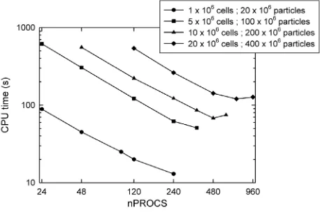
Fig. 3.Parallel performance of dsmcFoam+ for a lid-driven cavity case, showing the parallel speed-up for both strong and weak scaling.

the final mesh using the snappyHexMesh tool to refine the mesh in parallel. Other mesh refinement strategies, such as refineMesh could also possibly be utilised, but ultimately they need to be run in parallel across multiple nodes to have access to enough memory. Even more important than mesh generation is the particle initialisation phase. For particle numbers in the order of several hundred millions and more, initialisation must be performed in parallel usingXprocessors with ampirun -np X dsmcInitialise –parallelcommand. For this to work, domain decomposition using the decomposePar executable has to be performed before the case is populated with particles using the dsmcInitialise executable.

The parallel performance and scalability of the dsmcFoam+ code has been assessed on the ARCHER high performance computing system [38]. ARCHER is the UK’s national supercomputing service based around a Cray XC30 supercomputer, and was rated number 61 in the top 500 list of supercomputers published in November 2016. ARCHER compute nodes contain two 2.7 GHz, twelve core ES-2697 V2 (Ivy Bridge) processors, and have 64 GB of memory shared between the two processors. A weak scalability study has been carried out using a lid-driven cavity test case, considering 4 different cases of grid-size and particle numbers, i.e. 1 million cells with 20 million particles; 5 million cells with 100 million particles; 10 million cells with 200 million particles; and 20 million cells with 400 million particles. The Scotch domain decomposition method [39] is followed for this scalability study, in which all domains have approximately the same number of cells. The variation of wall-clock time taken for all cases is shown inFig. 3for up to 960 cores,nPROCS. The code performs reasonably well

for both increase in load and increase in number of MPI tasks for all the cases considered. The computational time is measured using the in-built OpenFOAM timing functionality and is the total time for the simulation to run to completion (this study was performed with a slightly older version of dsmcFoam+).

Run-time load balancing has also been introduced to dsmcFoam+, which the user controls in the[case]/system/balanceParDict and [case]/system/loadBalanceDictfiles. This enables the code to measure the maximum current level of parallel load imbalance,Lmax. Since

the move function (which performs the particle movements described in Section2.4) carries the largest computational overhead in dsmcFoam+, it is most efficient to ensure that each core has roughly the same number of particlesNprocto balance their loads. The ideal

number of particles on each coreNidealis thenN

/

nPROCS, whereNis the total number of DSMC particles in the simulation andnPROCSis the

number of processors the simulation is running on. At each write interval, the number of particles on each processorNprocis compared to

Nideal. If any of these fall outside a user-set tolerance (e.g. 0

.

9Nideal

<

Nproc

<

1

.

1Nideal) then the simulation is temporarily halted while the

domain decomposition is performed again to re-balance the load. Following this, the simulation automatically starts again from where it was stopped, using a bash script as shown below, where the user changes the final time directory (0.0004 in this example) to match that in their[case]/system/controlDictfile:

#!/bin/sh

cd ${0%/*} || exit 1

# run from this directory

while :

do

### Check that the final time directory does not exist ###

if [ ! -d "processor0/0.0004" ]

then

echo "Directory processor0/0.0004 DOES NOT exist, "\

"restart from the latest time."

mpirun -np 8 dsmcFoamPlus -parallel

else

echo "Directory processor0/0.0004 DOES exist, "\

"killing the script."

break ### exit the loop

fi

done

[image:8.595.102.506.55.191.2]

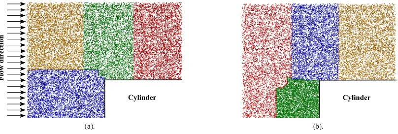
(a). (b).

Fig. 4.Final particle distributions in the cylinder case, coloured by processor number. (a) Simulation without load balancing, and (b) simulation with load balancing.

Bird’s case of axially-symmetric flow past a blunt-nosed cylinder (see [1], page 374) was used to demonstrate the effectiveness of the dynamic load balancing. This problem considers a flow of argon with a number density of 1

×

1021_m−3_{, a temperature of 100 K, and a}

velocity of 1000 m/s (i.e. Mach number of 5.37). The cylinder has a radius of 0.1 m and the domain extends 0.2 m upstream and downstream of the cylinder’s flat face, and 0.3 m radially. A constant DSMC cell size of 2.5

×

10−4_{m in the axial and radial directions was used, with a}

wedge angle of 5◦

in the symmetry direction. The cylinder surface was set at a constant temperature of 300 K and fully diffuse reflections were modelled. The time step was 8

×

10−8_{and each DSMC particle represented 1}

_×

₁₀10_{argon atoms. The radial weighting factor of}

1000.

First, Scotch decomposition [39] was considered and the simulation performed on 4 cores of a desktop workstation equipped with a dual threaded quad-core Intel⃝R

CoreTM_{i7–4770 CPU for 5000 time steps. Steady state was achieved after 1500 time steps, with around}

2.9 million DSMC simulator particles in the domain. During the run, dsmcFoam+ reported a maximum load imbalance of 44%, but load balancing was not activated; 3:59:15 hrs:mins:secs were required to complete the simulation. The simulation was then repeated, this time allowing a maximum imbalance of 5% before the load was rebalanced. This resulted in a reduced run time, including the time required to recompose and re-decompose the simulation, of 2:46:25 hrs:mins:secs. This is a speed-up of 30%, demonstrating the effectiveness of this technique for reducing run times on simulations involving density gradients that evolve as the simulation proceeds.Fig. 4compares the particle distributions, coloured by the processor that they belonged to when the simulation was complete, between the cases with and without load balancing. It is clear that the load balancing code has identified the stagnation region in front of the cylinder and concentrated processor power at this location, which has helped to reduce the computational time required to complete the simulation.

2.9. Extensible design

An important feature of dsmcFoam+ is its inherent ability to be extended. This capability was one of the key reasons OpenFOAM was originally selected as the base development framework. dsmcFoam+ is designed entirely in object-oriented C++and, in accordance with the OpenFOAM coding guidelines, the majority of its classes are therefore derived from existing OpenFOAM classes, primarily from the Lagrangian portion of the code. The result is that the typical design for all of the application’s modular elements is that a base class is provided (which often derives from a base OpenFOAM class) and a specialised class is then created to provide specific functionality.

Should it be desirable to add extra functionality to dsmcFoam+ then all that is required is to copy an appropriate specialised class, give it a new name, update the functionality, and then add the new class to the compilation list as per any other OpenFOAM addition. Once dsmcFoam+ is re-compiled the functionality provided by the new class can then be accessed by updating the appropriate line in the case dictionary files. While other DSMC codes may strive to provide this level of extensibility, the strict adherence of OpenFOAM (and therefore dsmcFoam+) to a fully object-oriented programming model means that any new addition made will perform as well as the code it is built upon. It also ensures a level of standardisation in any new addition and simplifies the process of adding new functionality.

The extensibility of dsmcFoam+ is also notable in the way cases are defined. Because the standard OpenFOAM case model is adopted, cases are specified as a series of input files, known as ‘‘dictionaries’’. These are plain text files that adopt a standardised format in which new variables can be defined by adding new text and a value associated with the name. Dictionary parsing is done within dsmcFoam+ using the basic OpenFOAM provided libraries, therefore the majority of variables used are free-form in nature (i.e. should new functionality be added that requires a new input parameter, this can be easily added to the corresponding dictionary file).

3. Downloading and installing dsmcFoam+

[image:9.595.180.406.55.286.2]

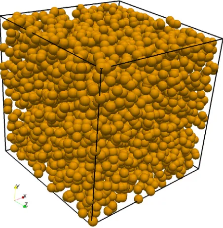
Fig. 5.DSMC simulation of argon in a cube of side lengthL, with specular walls applied at all boundaries.

4. Using dsmcFoam+

For those familiar with using an application within the OpenFOAM suite, usage of dsmcFoam+ will be relatively straightforward. However, in order to provide an illustrative example, the following section describes the process of defining, initialising, running (both in serial and parallel), and finally post-processing a simple case, consisting of a periodic cubic domain filled with argon at a temperature of 300 K and a molecular number density of 3

×

1020_m−3_.

This DSMC simulation is a canonicalNVTensemble, which means that it has a constant number of particlesN, a constant volumeV, and a constant temperatureT. The case can be seen inFig. 5; the domain consists of a periodic cubic box of side lengthL

=

0

.

6 m.

4.1. Case definition

Using dsmcFoam+ begins by creating a new DSMC case. As with other OpenFOAM applications, a dsmcFoam+ case has a typical file structure, therefore it is defined by first creating a new folder of an appropriate name (referred to henceforth as[case]), under which there are two more folders namedsystemandconstant. The former of these contains the majority of the OpenFOAM dictionary files which control most of the running parameters for the DSMC case (i.e. time-step control, case initialisation parameters, boundary conditions, etc.), while the latter contains details of the physical domain that is used to create and populate the underlying OpenFOAM mesh with particles. While there are some files within this structure that are specific to dsmcFoam+, they are named using typical nomenclature and are designed to be self-descriptive.

Alongside the example case described here, tutorial cases are also supplied within the software repository and can be found within the tutorials/discreteMethods/dsmcFoamPlusfolder.

4.1.1. Mesh creation

Simulations performed using dsmcFoam+ are defined in a three-dimensional Cartesian co-ordinate system and are most commonly processed using the blockMesh application (which is a base application within the OpenFOAM suite). While it is entirely possible, and sometimes desirable for complex three-dimensional geometries, to use one of the more advanced meshing tools that OpenFOAM provides, it is often sufficient to use blockMesh; therefore this will be described here.

The mesh is then used by a dsmcFoam+ simulation for a number of purposes: (a) to initially place particles; (b) to provide a cell-list algorithm for performing binary particle collisions; (c) to decompose a domain for parallel execution; and (d) to resolve macroscopic field properties from the underlying DSMC simulation.

1

/*---*\

2

| =========

|

|

3

| \\

/

F ield

| OpenFOAM: The Open Source CFD Toolbox

|

4

|

\\

/

O peration

| Version:

2.4.0-MNF

|

5

|

\\

/

A nd

| Web:

http://www.openfoam.org

|

6

|

\\/

M anipulation

|

|

7

\*---*/

8

9

FoamFile

10

{

11

version

2.4;

12

format

ascii;

13

14

root

"";

15

case

"";

16

instance

"";

17

local

"";

18

19

class

dictionary;

20

object

blockMeshDict;

21

}

22

23

// * * * * * * * * * * * * * * * * * * * * * * * * * * * * * * * * * * * * * //

24

25

convertToMeters 1;

26

27

vertices

28

(

29

(0 0 0)

30

(0.6 0 0)

31

(0.6 0.6 0)

32

(0 0.6 0)

33

(0 0 0.6)

34

(0.6 0 0.6)

35

(0.6 0.6 0.6)

36

(0 0.6 0.6)

37

);

38

39

blocks

40

(

41

hex (0 1 2 3 4 5 6 7) dsmcZone (60 60 60) simpleGrading (1 1 1)

42

);

43

44

boundary

45

(

46

walls

47

{

48

type wall;

49

faces

50

(

51

(1 2 6 5)

52

(0 4 7 3)

53

(2 3 7 6)

54

(0 1 5 4)

55

(4 5 6 7)

56

(0 3 2 1)

57

);

58

}

59

);

60

61

mergePatchPairs

62

( );

63

[image:11.595.198.384.54.237.2]

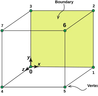
Fig. 6.Block structure of the cubic domain for the example case.

Referring to the example above, lines 1–24 are standard OpenFOAM dictionary header files. They are included in this first example for completeness, but are omitted from all further examples. Lines 27–37 define 8 vertices, which define one block on the mesh. In this simple case only one block is needed as the domain is a cube, therefore 8 vertices are all that is required. These vertices are numbered 0 to 7 and their physical locations are depicted inFig. 6. The valueconvertToMeterson line 25 allows the domain to be scaled, but in this case no scaling is applied and the vertex locations are given in metres.

Blocks are defined within theblocksregion; in this case, there is only one block that can be seen on lines 39–42, where the vertex order is first defined followed by the keyworddsmcZoneand thensimpleGrading. The entrydsmcZonedefines the number of cells to be created in thex,yandzdirections, which is written as

(

Nc,x

,

Nc,y

,

Nc,z

)

; the total number of cells that will be created isNc,x

×

Nc,y

×

Nc,z.

The cell size is therefore given by∆Li

=

Li

/

Nc,i, wherei

=

x

,

y

,

z; this is an important value when defining a DSMC simulation that uses

the cell-list algorithm, because ideally the cell size should be significantly smaller than the expected local molecular mean free path. The

simpleGradingparameter allows cells to be scaled in size in one or more directions, which can be useful if there is an obvious compression

region where the mean free path will be smaller, particularly in hypersonic flows.

The boundary entries shown on lines 44–58 indicate thepatchesthat form the domain’s boundaries. In this example of a periodic cube there is only one boundary, which is defined as a specular wall surface. Each patch contains the same two parameters:

1. patchName, which defines the type of the patch; this can be any viable OpenFOAM input, however it is most common to use either

patch(a generic boundary), orwall;

2. thefacesof a patch are defined by the vertices, e.g. here, the first face of the cubic domain is defined as being created by connecting vertex numbers one, two, six, and five, where the vertex numbering starts at zero.

Once the boundaries have been defined geometrically, it is also necessary to link the boundaries to the correct DSMC functionality, this is done within the file[case]/system/boundariesDictand for this example:

18

dsmcPatchBoundaries

19

(

20

boundary

21

{

22

patchBoundaryProperties

23

{

24

patchName

walls;

25

}

26

27

boundaryModel

dsmcSpecularWallPatch;

28

29

dsmcSpecularWallPatchProperties

30

{

31

}

32

}

33

);

34

35

dsmcCyclicBoundaries

36

(

37

);

38

40

(

41

);

42

43

// ************************************************************************* //

Each boundary has its parameters defined:boundaryModel, which specifies the type of model dsmcFoam+ will use, in this case the dsmcSpecularWallPatchclass has been selected. Other models exist within the application, such asdsmcDiffuseWallPatchclass, and new ones can be added by extending its capabilities. ThepatchNamelinks the names of the patches within theblockMeshDictwith the DSMC boundary models chosen.

Once these files are defined, the mesh and boundary data can be generated by running the OpenFOAM application blockMesh in the base of the[case]folder.

4.1.2. Particle properties

Constant particle properties can be set for each gas species involved in a simulation; these are defined in the dictionary file located at [case]/constant/dsmcProperties. An example of this file is:

19

// General Properties

20

// ~~~~~~~~~~~~~~~~~~

21

22

23

nEquivalentParticles

6.48e9;

24

25

// Axisymmetric Properties

26

// ~~~~~~~~~~~~~~~~~~

27

28

axisymmetricSimulation

false;

29

radialExtentOfDomain

0.03;

30

maxRadialWeightingFactor

1000.0;

31

32

33

// Binary Collision Model

34

// ~~~~~~~~~~~~~~~~~~~~~~

35

36

BinaryCollisionModel

LarsenBorgnakkeVariableHardSphere;

37

38

LarsenBorgnakkeVariableHardSphereCoeffs

39

{

40

Tref

273;

41

rotationalRelaxationCollisionNumber

5.0;

42

electronicRelaxationCollisionNumber

500.0;

43

}

44

45

// Collision Partner Selection Model

46

// ~~~~~~~~~~~~~~~~~~~~~~

47

48

collisionPartnerSelectionModel

noTimeCounter;

49

50

51

// Molecular species

52

// ~~~~~~~~~~~~~~~~~

53

54

typeIdList

(Ar);

55

56

moleculeProperties

57

{

58

Ar

59

{

60

mass

66.3e-27;

61

diameter

4.17e-10;

62

rotationalDegreesOfFreedom

0;

63

vibrationalModes

0;

64

omega

0.81;

65

alpha

1.0;

66

characteristicVibrationalTemperature

(0);

67

dissociationTemperature

(0);

68

ionisationTemperature

0;

70

Zref

(0);

71

referenceTempForZref

(0);

72

numberOfElectronicLevels

1;

73

degeneracyList

(1);

74

electronicEnergyList

(0);

75

}

76

}

Line 23 defines how many real gas atoms or molecules each DSMC particle represents. Properties for axi-symmmetric simulations are set on lines 28–30, but this example does not utilise this feature, hence line 28 is set

false. The binary collision model to be used when

two particles are accepted for collision is defined on line 36, with the user-defined properties for this model set on lines 38–43. The model to decide how many collisions to attempt in each computational cell is defined on line 48; in this case, Bird’s no-time-counter model is used but others, such as Stefanov’s simplified Bernoulli trials [29], are also available in dsmcFoam+.

Line 54 shows the definition of a new species of molecule in the form of atypeIdList. Each species should be given a unique name within this list (in this case there is only one, for argon). The index of each unique name within this list is used within dsmcFoam+ as a unique identifying number in order to keep track of different species types, in this caseAris given an ID of 0.

The physical properties of all species of molecule are defined between lines 56–76. Note, the properties of each species must be defined in the order they are listed in thetypeIdList.

4.1.3. Time control

The correct choice of time-step is fundamental to achieving a reliable DSMC simulation. A time-step that is too small will make the simulation too computationally expensive, while a time-step that is too large may cause an unrealistic transfer of mass, momentum, and energy during the collision routine, and cause particles to travel an unreasonable distance during the move function.

All controls associated with time-stepping, simulation length and file output are held in a single dictionary located at[case]/system/ controlDict, which is standard in OpenFOAM. An example of this file for the exemplar case is as follows:

17

application

dsmcFoamPlus;

18

19

startFrom

startTime; //Start simulation at startTime (available: latestTime)

20

21

startTime

0.0; //Start from 0 time (can be changed to any time)

22

23

stopAt

endTime; //End at endTime (other options available)

24

25

endTime

0.001; //Stops simulation when time has reached this value

26

27

deltaT

1e-06; //Size of DSMC time-step

28

29

writeControl

runTime;

30

31

writeInterval

1e-03; //File write interval

32

33

purgeWrite

3; //Only last 3 times are stored (0: no deletion)

34

35

writeFormat

ascii; //Format can be ASCII or Binary

36

37

writePrecision

10; //Floating point precision to write

38

39

writeCompression uncompressed; //Files can be compressed upon write

40

41

timeFormat

general;

42

43

timePrecision

6;

44

45

runTimeModifiable yes;

46

47

adjustTimeStep

no;

48

49

nTerminalOutputs 10;

and without chemical reactions) to be restarted following the same basic initial state. The nature of this functionality is best described in the OpenFOAM user-guide, but it involves setting the value ofstartTimeequal to an existing time folder containing a valid set of DSMC data. For a case set to start att

=

0, the initial values are stored in a folder located at[case]/0and the values are created using a separate pre-processing tool described in Section4.2.

The total number of time-steps taken is controlled by the value ofendTime, however it is important to remember that a DSMC simulation has a significant computational cost. Therefore, while it is normally desirable for the simulated time to be as long as possible, it is sensible to minimise the value ofendTimeto as few time-steps as are needed for an acceptable level of statistical scatter to be achieved. Another important consideration is how often to write data to disk. While it is possible for data to be written at every time-step (by settingwriteIntervalequal todeltaT), this should be avoided if possible as it will introduce significant processing overhead; for each time-step written, a new output folder has to be created and a number of individual files written out to disk within the new folder. This can have a significant impact on the final size of the case directory, especially in a typical DSMC scenario where the simulation may be run for hundreds of thousands of time-steps. Often the important values obtained from the simulation are time-averages, and not exact particle details at one point in time. It is therefore important to select appropriate values for how often data is output, and also how often historical data is deleted. This is controlled by thepurgeWritevalue, which in this case will ensure only the last 3 time-steps written remain on disk. For performance reasons, however, even when disk space is not an issue, the output frequency should still be controlled. Setting the value ofpurgeWriteequal to 0 will ensure all historical data will remain and the file-system overhead of deleting directories will not be incurred. An important additional point is that the value ofwriteIntervalshould be an exact integer factor of the time-step sizedeltaT.

A useful piece of functionality provided by dsmcFoam+ is the ability to modify the running state of an active DSMC simulation by editing the case’s controlDict file, so it ends cleanly without the process having to be killed by the user. This can be most useful when running a long case on an HPC resource where it is perhaps becoming obvious that a simulation has been initially set to run for longer than is actually required (i.e. perhaps it has reached steady-state more quickly than anticipated). In this case, the value ofstopAtcan be edited to equal eitherwriteNow, which will make it stop after completing the current time-step being calculated, or it can be set tonextWrite, which will make it stop following the next write-interval.

4.2. Case initialisation

Once all of the dictionary files to define a new case are in place and the underlying mesh has been created, as per Section4.1.1, it is then necessary to create an initial state for the DSMC simulation to evolve from. This is done using a pre-processing tool called dsmcInitialise, which, like dsmcFoam+ itself, is designed to be extensible to allow new initialisation algorithms to be implemented.

For the example case presented here, the goal is to insertNargon particles into the cubic domain in order to satisfy a target number density ofn

=

3

×

1020_m−3_{atoms, target temperature of 300 K, and target macroscopic velocity of 0 m/s.}

dsmcInitialise is controlled using a dictionary file located at[case]/system/dsmcInitialiseDict, the file for the example case is:

19

configurations

20

(

21

configuration

22

{

23

type

dsmcMeshFill;

24

25

numberDensities

26

{

27

Ar

3e20;

28

};

29

30

translationalTemperature

300;

31

rotationalTemperature

0;

32

vibrationalTemperature

0;

33

electronicTemperature

0;

34

velocity

(0 0 0);

35

}

36

);

As the example presented only has one species (argon, Ar), there is only one configuration entry in the above file, which refers to the correct molecules according to the pre-defined valuetypeID(see Section4.1.2). Should multiple species be involved, then one entry for each would be required. In this case the initialisation algorithm being used is thedsmcMeshFillclass, which fills the entire computational domain with particles with properties that will, on average, recover the desired density, temperature, and velocity.

When initialising a case, the main rule to follow is to ensure that there are enough DSMC particles in each computational cell to enable accurate collision statistics to be recovered. For the no-time-counter method, this requires at least 20 particles per cell. In this example test case, many more particles than that are used, but the following calculation of the expected number of particles in each cell is generally used to help decide the value ofnEquivalentParticlesin Section4.1.2that should be set. In this example, the cell volume is uniform at 1

×

10−6_m3_{. A molecule number density of 3}

_×

₁₀20_m−3_{andnEquivalentParticlesof 6.48}

_×

₁₀9_{gives a theoretical total of 46}

_,

₂₉₆

_.

₃

particles per cell. The dsmcInitialise tool will only create an integer number of particles, and uses a random fraction to decide if 46,296 or 46,297 particles will be created in each cell.

4.3. Running dsmcFoam+

Once all dictionary files have been created and the case initialised with the appropriate pre-processing tools, as described in Sections4.1.1and4.2, it is then possible to start the DSMC calculations in serial straight away. As the name suggests, this will perform all execution using a single dsmcFoam+ process.

While a serial run may be suitable for a small DSMC simulation, it is usually preferable to make use of multiple processors wherever possible. As dsmcFoam+ utilises MPI based domain decomposition, this can be accomplished on a workstation with a few CPU cores or on a large distributed memory system over hundreds or even thousands of cores. In order to execute a dsmcFoam+ based case in parallel there is an extra pre-processing step needed. This is achieved using the OpenFOAM utility decomposePar, which reads a dictionary at[case]/system/decomposeParDict. The layout of this dictionary follows the OpenFOAM standard, therefore reference to the official documentation is encouraged. However, the most important consideration when decomposing large or complex domains is which algorithm to use. OpenFOAM provides access to a number of domain decomposition techniques — some its own, others provided by external libraries. The choice of which produces the best decomposition has to be made on a case-by-case basis.

When decomposePar is executed in the base of the case folder, it creates a number of new folders, one for each processor being executed upon. Each of these contains a working copy of the sub-set of the overall domain contained with the initialisation folder created in Section4.2.

Once the domain decomposition has been achieved, a parallel run of dsmcFoam+ can be initialised using the appropriate MPI run-time for the MPI library that was originally used during its compilation. An important point to note is that dsmcFoam+, like other OpenFOAM applications, must be informed that it is to run in parallel. This is done using a new switch passed through at the point of execution; an example of running 256 MPI ranks using a typical environment would be:

mpirun -np 256 dsmcFoamPlus -parallel

4.4. Post-processing results

One of the powerful features of building dsmcFoam+ from OpenFOAM is the post-processing and visualisation of results. By default, OpenFOAM provides a wrapper around the visualisation environment ParaView [19] (called paraFoam). This automatically loads all appropriate data of an OpenFOAM case into ParaView and sets up a work-flow within the tool to enable quick visualisation of results. It is important to note that this can be done at almost any time while data exists (i.e. it is possible to view an initialised DSMC case before any DSMC calculations are performed) by simply executing paraFoam in the base of the case folder. While it is beyond the scope of this document to provide full details of how to utilise ParaView to best effect, detailed instructions can be found within the documentation provided in the software release.

An alternative to running paraFoam is the utility foamToVTK. This processes the data and creates a new folder namedVTKin the case directory, the contents of which can be viewed in any visualisation package that supports the VTK format.

If results have been generated by a parallel run of dsmcFoam+, then only a portion of the whole domain will be contained within each processor folder that resides within the overall case folder. It is possible to reconstruct the whole domain for each stored time-step using the OpenFOAM reconstructPar utility, or to treat each set of results independently. However it is important to ensure any processing tool is called from the base of the correct folder (i.e. if paraFoam was executed in the base of the case folder before reconstructPar was executed then this would be invalid).

4.5. Source code structure

As dsmcFoam+ is distributed as part of a customised OpenFOAM repository, the structure of its source code and that of any associated processing applications is in line with other applications built within OpenFOAM. It is beyond the scope of this article to describe the OpenFOAM coding style, therefore it is recommended that the OpenFOAM documentation is first reviewed in order to understand the general source-code structure. The remainder of this section assumes a level of understanding on the part of the reader in terms of how OpenFOAM organises its applications and classes.

As with all OpenFOAM applications, the source code for dsmcFoam+ and its associated processing tools are located in two base folders within the general repository directory. The applications themselves can be found in theapplicationsfolder while the underlying C++ classes can be found in thesrcfolder. In terms of applications, dsmcFoam+ can be found inapplications/discreteMethods/dsmc/dsmcFoamPlus while associated processing applications can be found inapplications/utilities/preProcessing/dsmc. Underlying classes can be found in src/lagrangian/dsmc.

Detailed documentation is also included with the repository, providing both installation instructions for a general workstation with a POSIX environment as well as in-depth technical detail. These can be found in thedocfolder, located atdoc/MicroNanoFlows.

Finally, tutorial example cases are also provided, these can be found within thetutorialsfolder, located attutorials/discreteMethods.

5. Validation

In this section, four examples that validate dsmcFoam+ against analytical solutions and other DSMC codes are presented.

5.1. Collision rates

[image:16.595.119.485.74.106.2]

Table 2

Number densities for the collision rate test simulations.

Case nO₂(m−3_{) nN}

2(m

−3₎

I 1×1019 ₀

[image:16.595.121.485.141.192.2]

II 1×1019 _1×1019

Table 3

Molecular properties for the collision rate test simulations.

O2 N2

Tref(K) 273 273

dref(m) 4.07×10−10 _4.17×10−10

m(kg) 53.12×10−27 _46.5×10−27

[image:16.595.126.484.222.451.2] [image:16.595.121.485.224.449.2]

ω 0.77 0.74

Table 4

Simulated collision rates compared with analytical values for an oxygen–nitrogen mixture.

Temperature (K) Simulated/analytical rate % Error

3,000 1.0000 0.0035

5,000 0.9998 0.0225

10,000 0.9995 0.0462

15,000 0.9994 0.0610

20,000 0.9993 0.0693

25,000 0.9995 0.0467

30,000 0.9995 0.0522

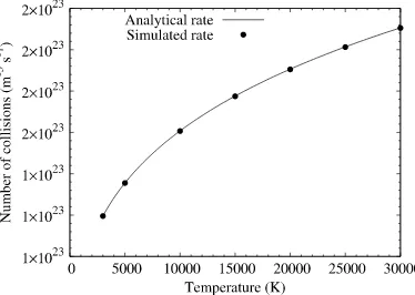
Fig. 7.Collision rate variation with temperature for Case I, pure oxygen. dsmcFoam+ results are compared to the analytical solution of Eq.(17).

collision rates. In the following simulations, the particles do not move and they do not collide; however, the probability of them colliding is still calculated and if the collision is ‘accepted’, a counter is updated, enabling collision rates to be measured for an equilibrium system with no gradients.

Both of the cases are of a single-cell simple adiabatic box. The cell is cubic with a volume of 1.97

×

10−5_m3_{, and the time step employed}

for all cases is 1

×

10−7_{s. Each DSMC simulator particle represents 2}

_×

₁₀8_{real gas molecules. The molecule number densities and gas}

species (oxygen and nitrogen) for each case are outlined inTable 2, with the molecular properties being given inTable 3. Case I contains around 1 million DSMC particles and Case II has around 2 million. The number of collisions is counted for a total of 1000 time steps in all cases.

We compare the equilibrium collision rates

(

Npq

)

0calculated by dsmcFoam+ to the exact analytical expression as given in Equation

(4.78) of Bird [1], i.e.:

(

Npq

)

0

=

2

π

1 2

(

_dref

)

2

pqnpnq

{

T

/(

Tref

)

pq

}

1

−ωpq

_{

_2k

B

(

Tref

)

pq

/

mr

}

1

2

,

₍₁₇₎

wherep andqrepresent different species and the subscript 0 denotes equilibrium quantities,dref,Tref and

ω

are the variable hard

sphere parameters for reference diameter, reference temperature and viscosity exponent, respectively,nis the number density,kB is

the Boltzmann constant,Tis temperature, andmris reduced mass. Eq.(17)returns the number of collisions per unit volume per second,

although it double counts because it calculates collisions betweenpqandqp; therefore, if a same species collision calculation is being performed it is necessary to include a factor of a half in order to achieve the correct rate.

Fig. 7shows the analytical rate for Case I, pure oxygen, compared with the results from the dsmcFoam+ simulation. Excellent agreement is found between the simulated and analytical rates, indicating that the no-time-counter model implemented in dsmcFoam+ returns collision rates that are in agreement with theory for an equilibrium, single species gas.