The Environment Review 2012

John Curtis

June 2012

Environment Review

2012

Environment Review 2012

John Curtis

RESEARCH SERIES

NUMBER 26

June 2012

Available to download from

www.esri.ie

© The Economic and Social Research Institute

Whitaker Square, Sir John Rogerson’s Quay, Dublin 2

The ESRI

The Economic Research Institute was founded in Dublin in 1960, with the assistance of a grant from the Ford Foundation of New York. In 1966 the remit of the Institute was expanded to include social research, resulting in the Institute being renamed The Economic and Social Research Institute (ESRI). In 2010 the Institute entered into a strategic research alliance with Trinity College Dublin, while retaining its status as an independent research institute.

The ESRI is governed by an independent Council which acts as the board of the Institute with responsibility for guaranteeing its independence and integrity. The Institute’s research strategy is determined by the Council in association with the Director and staff. The research agenda seeks to contribute to three overarching and interconnected goals, namely, economic growth, social progress and environmental sustainability. The Institute’s research is disseminated through international and national peer reviewed journals and books, in reports and books published directly by the Institute itself and in the Institute’s working paper series. Researchers are responsible for the accuracy of their research. All ESRI books and reports are peer reviewed and these publications and the ESRI’s working papers can be downloaded from the ESRI website at www.esri.ie

The Author

John Curtis is an environmental economist at the Economic and Social Research Institute.

Acknowledgements

Table of Contents | v

Table of Contents

Executive Summary ... vii

CHAPTER 1: INTRODUCTION ... 1

CHAPTER 2: TRENDS IN THE ECONOMY ... 3

CHAPTER 3: ENVIRONMENT ... 5

CHAPTER 4: DISCUSSION AND CONCLUSION ... 23

Appendix 1: The ESRI Environmental Accounts ... 27

Appendix 2: Ireland’s Sustainable Development Model (ISus) ... 33

Executive Summary | vii

Executive Summary

The Environment Review 2012 presents projections of environmental emissions covering the period to 2030. The projections, which are based on current policies, provide a baseline of projected emissions (e.g. greenhouse gases, waste generation) to which the effects of any new policy can be compared. We highlight areas where government intervention, in addition to current policies, is required to meet committed targets and avoid environmental damage, concentrating on the areas of greenhouse gas emissions, the expansion of agricultural output and waste management.

The projections presented in this report are based on a series of environmental and economic models. Ireland’s Sustainable development model (ISus) was used to develop environmental emissions projections. ISus is a simulation model that combines behavioural equations to predict future levels of environmental emissions. The current version of the model uses data for the period 1990-2009/10 for calibration and to estimate behavioural relationships, while projections are generated for the period 2010/11-2030. ISus covers a range of potential pollutants (to air, water and waste) emanating from 20 sectors of the economy, including the residential sector. Underlying the environmental figures are a number of model projections on population growth, domestic and international economic growth, energy and carbon markets. The most important of these is the scenario developed using the ESRI’s macroeconomic model, HERMES. This provided the economic data upon which the ISus emissions projections are based. Medium-term economic projections in the current period of uncertainty in the euro area are fraught with difficulty. Though subject to considerable uncertainty we present emissions based on just one economic projection. That underlying economic scenario may be overly optimistic, especially in the short term; for instance it is much more favourable on the short term outlook than the ESRI’s Quarterly Economic Commentary. Regardless of timing, a growing population and an expanding economy, when recovery firmly takes hold, will potentially lead to growing pressure on the environment through increased emissions and waste generation once the EU economy recovers; and the purpose of this report is to highlight where these environmental pressures are likely to arise.

viii| Environment Review 2012

may differ from those produced elsewhere. For example, our greenhouse gas emissions’ projections contrast significantly with EPA (2012), as we are less optimistic than the EPA about the effectiveness of existing and planned policy measures at reducing emissions.

Compliance with Greenhouse Gas Emissions Targets: Coinciding with the recession there was a dramatic decline in greenhouse gas emissions and there is now a general consensus that Ireland’s actual emissions will comply with its Kyoto Protocol target of 314.18 Mt CO2eq for the five-year commitment period

2008-2012.∗ _{While at a national aggregate level Ireland is likely to achieve}

compliance with the Kyoto target, it is worth noting that emissions from non- Emissions Trading Scheme (ETS) sources will still exceed their allocated share. Compliance with longer term targets, such as Ireland’s contribution to the EU’s 20-20-20 climate and energy target, will be much more difficult. Ireland’s target is a 20 per cent reduction in non-ETS emissions compared to 2005. For the economy as a whole (ETS and non-ETS sectors) we project a small growth in emissions to 2020, averaging 1.4 per cent per annum in the period 2015-2020. Within the ISus model it is difficult to disentangle ETS emissions from the rest of the economy but we expect that non-ETS emissions could be as much as 5 per cent higher than 2005 levels in 2020. Without significant policy intervention we project actual emissions will substantially exceed the policy target.

Emissions Trading System: The EU-ETS regulates installations emitting large quantities of greenhouse gases, whereas the carbon tax and other instruments are used to curtail emissions in the rest of the economy. One area that offers some scope for emissions reduction crosses both the ETS and non-ETS sectors is fuel switching. In 2010 peat accounted for 5.4 per cent of the total primary energy requirement of the state and 10 per cent of the electricity-generation fuel mix but it contributes more than double the amount of CO2 emissions per unit

energy compared to gas and nearly 60 per cent higher than oil. The phase out of peat in electricity generation (which is already declining) would make a contribution to emissions reduction without significant negative impact on competitiveness (though this would not contribute to non-ETS emissions targets), whereas extending the carbon tax to peat would discourage its use in the residential sector (e.g. peat briquettes). A phase out of peat as a fuel would reduce greenhouse gas emissions and there would be a significant additional benefit through a reduction in particulate emissions, which have an adverse impact on health.

Executive Summary | ix

Food Harvest 2020: Agriculture accounts for 30 per cent of national total

greenhouse gas emissions, the highest share for any sector. Emissions from the sector have declined by 2 million tonnes over the past decade but full implementation of Food Harvest 2020 strategy will reverse that trend. We project that implementation of the strategy will increase emissions from livestock by 1 million tonnes by 2020. It might be assumed that agriculture is no different than any other sector and that it should be expected to curtail its emissions in line with other sectors of the economy. However, agriculture is a special case in that, if climate policies curtail Irish milk and beef production, production will move overseas to places like Brazil, without any global environmental benefit. Preserving emissions-efficient production within Europe would be preferable. Consideration should therefore be given to seeking, at EU level, a special mechanism for managing agricultural emissions within Europe. Ireland has a comparative advantage in beef and dairy production and has the potential to expand output and employment; however, the current mechanism for managing emissions within the sector is a threat to realising those benefits.

Industrial Sector: One area where we project potential future environmental pressure is in emissions of so-called F-gases, which are particularly potent greenhouse gases emitted in industrial production processes. To date these emissions have not been a particularly pressing issue, as they have represented such a small share of total emissions. Based on historical emission intensities, we project that emissions from this source could grow such that their share of total greenhouse gas emissions could increase from 1 per cent at present to over 4 per cent within a decade. The current review of the European regulation on F-gas emissions is an opportune time to amend current controls and prevent substantial emissions growth from occurring.

x| Environment Review 2012

Water Quality: Food Harvest 2020, the development strategy for the agri-food sector, proposes a substantial expansion in output and employment. The strategy could have significant impact on the environment in terms of greenhouse gas emissions and potential nutrient emissions to water. The strategy’s plan to expand dairy production by 50 per cent will increase greenhouse gas emissions, which was discussed earlier, and will also significantly increase the amount of nutrients generated by livestock, which must be managed to prevent environmental damage. We project that an additional 22,000 tonnes of excreted nitrogen will be produced in 2020 compared to a no-strategy baseline. Based on current levels of production, and with many surface and ground waters already subject to high levels of nutrient enrichment, existing nutrient management practices are likely to be inadequate to protect the environment from further harm under a scenario of expanding production. Protecting water quality from diffuse pollution sources is extremely difficult but nutrient sources, whether from agriculture or elsewhere, should be able to demonstrate that their activities are not causing environmental damage. The establishment of a system to verify implementation of best practice for nutrient management within agriculture would assist expansion in the sector while protecting environmental quality.

Waste Management: Waste generation from the household and commercial sectors has been declining since 2006/07 and, with the effects of the recession lingering, in particular high unemployment, the downward trend in waste generation is expected to continue. In the case of household waste we expect that the downward trend will continue to 2015. With a recovery in the economy, increased employment, as well as projected growth in the population, we anticipate waste generation to be substantially higher in the future than today. By 2030 we project that municipal waste generation will be 33 per cent or roughly 0.9 million tonnes higher than current levels. In the case of households we project waste generation will be 24 per cent higher than current levels. The return to growth in waste generation will have an impact on the waste management sector in terms of future collection and treatment capacity. Regional waste management plans, which are currently being reviewed, will need to be updated to reflect anticipated growth in waste streams.

Executive Summary | xi

Introduction | 1

Chapter 1

Introduction

In 1987, 25 years ago, unemployment and sovereign debt dominated public discourse. Much has happened since then, including the return of these issues to the centre of public debate. However, in the intervening period the issues of environmental degradation and climate change have steadily risen up policy agendas both domestically and internationally. The growing focus on the environment, including climate, stems from better knowledge of how the environment, the productive economy and societal well-being are interdependent. It is now widely acknowledged that many major environmental problems are not cyclical events or natural phenomena but directly linked to human activity. For example, the collapse in bee populations, which pollinate many of the world’s crops, has been linked to commonly used pesticides (Whitehorn et al., 2012; Henry et al., 2012). Furthermore, climate change, which has the potential to dramatically (even catastrophically) affect habitats and societies globally, has been linked to the growth in carbon dioxide emissions from human activity since the industrial revolution (IPCC, 2007). While current emissions are monitored and regulated to prevent environmental harm, the confluence of a growing population, an evolving economy and a changing environment (e.g. climate change) means that the pressures on the environment are continually transforming. The development of environmental scenarios helps us to understand where future environmental pressures are likely to be greatest and informs environmental policy discourse in relation to what are the issues that need to be tackled.

2 |Environment Review 2012

This is the fourth Environment Review published by the Economic and Social Research Institute. The first two editions ( Fitz Gerald et al., 2008; Bergin et al., 2009) were part of larger publications, whereas the third edition (Devitt et al., 2010) also encompassed a review of energy. TheEnvironment Review is not the only source of scenarios for the environment, as the Environmental Protection Agency (EPA) regularly publishes its outlook on greenhouse gas emissions (EPA, 2012), while the Central Statistics Office (CSO, 2012) has begun a biennial environmental indicators report. The Environment Review distinguishes itself from these publications in two ways: its scenarios include the impact of policies, and it discounts any government targets that are supported by few measures or reasoning as to how they will be attained. The EPA also publishes its State of the Environment report (EPA, 2008) every four years, which has a much wider brief covering topics such as biodiversity, soils, and chemicals. While The Environment Review addresses a range of current topical issues it does not discuss the full spectrum of environmental issues.

Trends in the Economy | 3

Chapter 2

Trends in the Economy

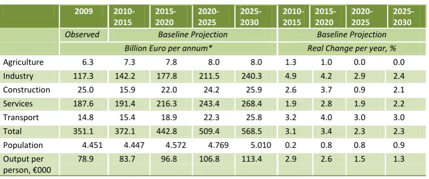
Our environmental emissions projections rely on an assumed scenario for economic growth, which was compiled by the ESRI in October 2011 and is based on the low-growth scenario in Bergin et al. (2010) with a number of updated assumptions on government finances and with the international outlook based on the National Institute of Economic and Social Research’s (NIESR) July 2011 Review. The main domestic macroeconomic projections are presented in Table 2.1, which shows that the economy is projected to gradually recover from the recession and reach moderate levels of growth within the next few years. Recovery in the construction sector is projected to take somewhat longer but a return to growth is anticipated by 2014-15. Total economic output is projected to grow by on average approximately 3 per cent per annum over the coming decade. This contrasts with short-term forecasts, such as Duffy et al. (2012), who forecast significantly lower growth in the period to 2013.

Table 2.1: Economic Gross Output and Population as Observed and as Projected

2009

2010-2015 2015-2020 2020-2025 2025-2030 2010-2015 2015-2020 2020-2025 2025-2030

Observed Baseline Projection Baseline Projection Billion Euro per annum* Real Change per year, %

Agriculture 6.3 7.3 7.8 8.0 8.0 1.3 1.0 0.0 0.0 Industry 117.3 142.2 177.8 211.5 240.3 4.9 4.2 2.9 2.4 Construction 25.0 15.9 22.0 24.2 25.9 2.6 3.7 0.9 2.1 Services 187.6 191.4 216.3 243.4 268.4 1.9 2.8 1.9 2.2 Transport 14.8 15.4 18.9 22.3 25.8 3.2 4.0 3.0 3.0 Total 351.1 372.1 442.8 509.4 568.5 3.1 3.4 2.3 2.3 Population 4.451 4.447 4.572 4.769 5.010 0.2 0.8 0.8 0.9 Output per

person, €000 78.9 83.7 96.8 106.8 113.4 2.9 2.6 1.5 1.3 * Billion Euro with the exception of Population (million) and Output per person (€000).

Source: after (Bergin et al., 2010).

4 |Environment Review 2012

Environment | 5

Chapter 3

Environment

Ireland’s Sustainable development model (ISus) was used to develop the environmental emissions projections presented in this report. ISus is a simulation model that combines behavioural equations to predict future levels of environmental emissions. The current version of the model uses data for the period 1990-2009 (the period covered by the ESRI Environmental Accounts) to calibrate the model and estimate behavioural relationships, while projections are generated for the period 2010-2030.1

ISus covers in excess of 70 substances and potential pollutants (to air, water and waste) emanating from 19 NACE2 _{productive sectors, as well as the}

residential sector. Further details about the ESRI Environmental Accounts and the ISus model are contained in Appendices to this report.

3.1 G

G

E

Climate change continues to be a pressing environmental policy issue with a range of European and international targets aimed at significantly reducing emissions. Table 3.1 shows greenhouse gas emissions, per gas and sector, observed in 2009 and projected trends until 2030. For much of the period since 1990 greenhouse gas emissions grew at an average of 1 per cent per annum but coinciding with the recession there was a dramatic decline in emissions and our projection is that total emissions will not rise substantially above 2009 levels before 2020. Consequently it is likely that Ireland’s actual emissions will comply with its Kyoto Protocol target of

314.18 Mt CO2eq for the five-year commitment period 2008-2012.4

However, it is likely that emissions from non-Emissions Trading Scheme (ETS) sources will exceed their share of the national target.5 _Compliance

with a second Kyoto commitment period, as agreed in the Durban Platform

1 _{In the case of waste, historical data include 2010 and projections cover 2011-2030.} 2 _{The NACE code system is the European standard for industry classifications.}

3 _{The analysis on greenhouse gas emissions is based on historical data from 1990-2009 and completed prior to the}

Environmental Protection Agency’s publication of greenhouse emissions for 2010.

4 _{This equates to an average of 62.84 Mt CO}

2eq per annum over the period (i.e. 13 per cent above the baseline

estimate).

5 _{The ETS is the cornerstone of the EU’s policy to combat climate change and covers in excess of 11,000 large scale}

6 |Environment Review 2012

in December 2011,6 _{will be more difficult without resort to buying}

allowances to offset the projected emissions in the period to 2020. Compliance with the EU’s 20-20-20 targets will be much more onerous. The EU 20-20-20 target requires greenhouse gas emissions reductions of at least 20 per cent below 1990 levels for the EU by the year 2020, which compares to Ireland’s target of the first Kyoto commitment period (2008-2012) of 13 per cent above 1990 levels (which will roughly match emissions during that period). The target for Ireland under EU 20-20-20 is a 20 per cent reduction in non-ETS emissions compared to 2005. Our projection for the combined ETS and non-ETS sectors (i.e. the entire economy) is a small growth in emissions over that time period, as shown in Table 3.1. Within the ISus model it is difficult to disentangle ETS emissions from the rest of the economy but we expect that non-ETS emissions could be as much as 5 per

Table 3.1: Greenhouse Gas Emissions as Observed and as Projected Per Gas and Per Sector

2009

2010-2015 2015-2020 2020-2025 2025-2030 2010-2015 2015-2020 2020-2025 2025-2030

Observed Baseline Projection Baseline Projection

Million tonnes CO2eq per year* Change per year, %

CO2, energy 40.9 40.4 44.2 46.4 49.8 1.0 1.9 0.5 1.9

CO2, process 1.6 0.9 1.1 1.0 0.9 -0.7 0.3 -2.3 -1.4

CO2, land use -2.3 -2.6 -3.7 -4.5 -5.4 7.3 4.8 3.9 3.2

CH4** 12.0 11.6 11.4 11.4 11.4 -1.1 0.2 0.0 0.0 N2O 7.2 7.1 6.9 6.9 6.7 -1.6 0.2 -0.4 -0.4 F-gases 0.6 1.0 1.6 2.5 3.8 11.5 10.3 8.7 7.8 Agriculture*** 18.2 17.8 17.6 17.6 17.5 -1.0 0.3 -0.1 -0.1 Industry 16.9 17.9 19.5 20.1 22.3 1.6 1.9 0.3 3.2 Construction**** 3.2 1.9 2.4 2.5 2.5 0.9 2.2 -0.4 0.9 Services 3.2 3.1 2.9 2.9 2.9 -1.9 -0.1 -0.2 0.4 Transport 13.1 13.0 15.1 17.0 18.9 1.9 2.9 2.1 2.2 Residential 7.5 7.2 7.6 8.1 8.4 -0.5 2.0 0.7 1.0 Total (incl. sinks) 59.9 58.3 61.6 63.7 67.2 0.1 1.4 0.4 1.6

* Levels are in million metric tonnes of carbon dioxide equivalent, using the IPCC AR2 global warming potentials; CO2 = carbon dioxide; CH4 = methane; N2O = nitrous oxide;

F-gases = HFC23, HFC32, HFC34a, HFC125, HFC143a, HFC152a, HFC227ea, CF4, C2F6, cC4F8 and SF6; ETS = EU Emissions Trading Scheme.

** Note that methane emissions from landfill reported here differ from the official statistics. See section 3.2 for further discussion.

*** This baseline scenario excludes the Food Harvest 2020 strategy, which is discussed separately in section 3.5 below.

**** Note that cement production (an industry) and construction (a service) are listed together as construction. Source: ESRI Environmental Accounts and ISus.

6 _{The Durban Platform outcome states that the terms of a future treaty on climate change are to be defined by}

Environment | 7

cent higher than 2005 levels in 2020. These estimates contrast significantly with EPA (2012), which projects a decline in non-ETS emissions though not by as much as the 20 per cent target. The difference between projections is due to differing underlying assumptions. We are not as optimistic as the EPA about the effectiveness of existing and planned policy measures at reducing emissions. We do not necessarily assume that policy targets will be achieved, such as the 20 per cent improvement in energy efficiency across all sectors, the 40 per cent renewable electricity (RES-E) share target and the 10 per cent renewable transport (RES-T) share target (including 10 per cent electric vehicles penetration target). Rather than impose certain outcomes we have modelled what we believe the most likely outturn based on current policies. For example, in transport we project a substantial growth in emissions – a higher population, more cars and more travel offsetting efficiency gains. In agriculture our underlying livestock population projections differ; Teagasc supplied EPA with data in December 2011, whereas we rely on older published Teagasc data (Donnellan and Hanrahan, 2011).

Figure 3.1: Greenhouse Gas Emissions by Gas and Policy Targets

* The graph shows the agreed target under the Kyoto Protocol for 2008-2012, and for the period 2013-2020 the annual non-ETS target plus an assumed (constant) ETS emissions (equal to projected annual ETS emissions for Kyoto Period of 17.8 million tonnes, (EPA, 2012)).

8 |Environment Review 2012

Though we project total emissions to only grow slightly we expect the relative composition of emissions to change considerably, as has been the case for the past two decades. We project that beyond 2020 the industrial sector will be responsible for the greatest share of emissions, surpassing agriculture (excluding sinks).7 _{This is partly due to our projection of F-gas}

emissions and is discussed later. Agriculture will continue to be a major source of emissions, though its level of emissions has been gradually declining since 1999. A resumption of growth in transport emissions is projected, with its share of emissions rising by 5 percentage points over the next two decades. The dramatic decline in emissions from construction is expected to continue from a 7 per cent share of total emissions in 2004/05 to approximately a 3-4 per cent share for the next 10-15 years. Climate policy will have to adapt to these changes in emission sources and concentrate efforts to curtail emissions where they are rapidly expanding, for example in transport.

In the industrial sector we project a strong growth in emissions of F-gases, where we assume an emissions profile based on historical emissions intensity. To date the growth in these emissions have not been a particularly pressing issue, as they have represented such a small share of total emissions. If emissions continue to grow as projected their share of total greenhouse gas emissions will steadily increase from 1 per cent at present to over 4 per cent within a decade. While policy is prudently targeted at the other greenhouse gases, which account for the majority of emissions, it would be wise to closely monitor developments in this emission source and intervene, as necessary, to offset any dramatic growth in this source of greenhouse gas emissions. The current review of Regulation (EC) No. 842/2006 on fluorinated greenhouse gases (F- gases) is an opportunity to ensure that the existing regulatory framework is adjusted to curb any significant growth in F-gas emissions.

Emission sinks from land use change, essentially forestry, are becoming an increasingly important resource in reducing national greenhouse gas emissions. In 2010 forest sinks totalled 3 million tonnes CO2eq or roughly 5

per cent of total national emissions. Within ten years we project that land-use sinks will double in magnitude. The benefits of these sinks, which are being realised now, are due to forestry policy in the 1990s and 2000s that subsidised new forestry plantations. The continuation of these benefits in

7 _{For industry sectors we follow the industrial NACE classifications. The official greenhouse gas inventory and}

Environment | 9

the longer term depends on existing plantations being re-planted once clear felled, and it is immensely important to ensure that this land, much of it in relatively small parcels, continues in forestry production past its first rotation. Other potential land-use sinks, such as croplands or grasslands are not included, though it is also worth noting that Land Use, Land Use Change and Forestation emissions are not included in the current targets regime at EU level.

3.2 M

E

L

Devitt et al. (2010) previously noted differences between ISus and EPA’s estimates of methane emissions from landfill, the latter of which is submitted to the UN Framework Convention on Climate Change. The ISus model for methane emissions from landfill continues to be updated in light of new information, for example data on flaring and landfill gas recovery.8 _In

November 2011 the EPA made revisions in its estimate of greenhouse gas emissions from landfill for the years 2007-2009 with reductions of between 11 and 23 per cent of their April 2011 estimate.9 _{These revisions have yet to}

been incorporated into the ISus model but the differences represent a small proportion of the total emissions.

3.3 W

The ESRI Environmental Accounts now distinguish five types of waste (hazardous, biowaste, BMW non-biowaste, other non-biowaste, and stone and soil – see Appendix 1 for more detail). From these five accounting categories we can aggregate to various waste types of policy interest, for instance, biodegradable municipal (BMW), municipal solid (MSW), construction (C&D), industrial, household, etc. The accounts distinguish between five waste destinations (landfill, recycle, incinerate, use as a fuel and unattributed). Unattributed waste is either waste that we do not know its sector of origin (e.g. some hazardous waste)10 _{or more usually waste that}

is not collected and managed within the waste management system. More detail on the waste categories and destinations are included in Appendix 1. With the commissioning of a municipal waste incinerator during 2011 we

8 _{Fehily Timony (2009) estimated methane recovered through landfill gas flaring for all years since the practice}

was introduced.

9 _{Ireland's Provisional Greenhouse Gas Inventory 1990-2010, published 9 November 2011,}

http://epa.ie/downloads/pubs/air/airemissions/name,30829,en.html, accessed 24/11/11; Ireland National Inventory Report 2011 Greenhouse Gas Emissions 1990-2009, http://coe.epa.ie/ghg/, accessed 25/11/11; and Common Reporting Format File IRL-2011-2009-v1.4.xls, http://coe.epa.ie/ghg/, accessed 25/11/11;

10 _{Although we may be unable to attribute certain wastes to a sector of origin that is not to say that the origin of}

10 |Environment Review 2012

have also changed how ISus projects utilisation of waste incineration capacity. Previously, we assumed that BMW would be prioritised for incineration, which was a convenient mechanism to investigate the minimum potential shortfall within the context of the Landfill Directive’s targets. We now assume that BMW and other MSW will be incinerated in proportion to its composition in residual waste, though we will adjust this further as information becomes available on the composition of waste incinerated. We also distinguish incineration ash as a secondary waste category to avoid double counting.

In this section we provide projections of future waste generation based upon macroeconomic activity and waste management policy scenarios. The macroeconomic projections date from October 2011, as discussed above in Section 2. Future research with the ISus model will investigate the sensitivity of emissions projections to underlying macroeconomic projections. The underlying waste management scenario assumes no change in policy since 2011. Given the review of national waste policy in 2011 it is likely that policy will be amended in the near future, so a scenario of no policy change provides a baseline of projected waste generation to which any new policy impacts can be compared.

Table 3.2: Waste Arisings as Observed, and Projected for Municipal Solid Waste (MSW), Biodegradable Municipal Waste (BMW), Household Waste, Biowaste, Hazardous Waste, and Construction and Demolition Waste (C&D)

2010

2010-2015 2015-2020 2020-2025 2025-2030 2010-2015 2015-2020 2020-2025 2025-2030

Observed Baseline Projection Baseline Projection

Million tonnes per year Change per year, %

MSW* 2.73 2.75 3.04 3.38 3.63 0.8 2.7 1.5 1.7 BMW* 1.80 1.83 2.02 2.25 2.43 0.9 2.7 1.6 1.8 Household

waste* 1.58 1.56 1.69 1.86 1.96 -0.1 2.7 1.2 1.2 Biowaste** 1.35 1.38 1.53 1.69 1.81 1.2 2.4 1.5 1.6 Hazardous 0.29 0.40 0.51 0.61 0.70 5.2 4.4 3.1 2.5 C&D

waste*** 3.34 3.39 4.09 3.91 3.55 4.2 -0.3 -1.8 -1.9

* Includes managed and uncollected.

** Biowaste projections exclude Harvest 2020 Strategy ambitions.

Environment | 11

Table 3.2 shows observed waste arisings11 _{for 2010 and projections for}

future periods to 2030. During the recession waste arisings declined across all sources and waste types with the most dramatic fall occurring in construction and demolition (C&D) waste. The decline in C&D waste is expected to continue through 2012, after which moderate growth is anticipated for the remainder of the decade. Hazardous waste is also anticipated to increase quite rapidly, though the total weight of hazardous waste is significantly lower than that managed during the height of the construction boom when the greater share of hazardous waste comprised of contaminated soil. The remaining four waste categories in Table 3.2 are inter-related. The majority of municipal waste (MSW) is biodegradable (BMW) and the majority of BMW comprises biowaste but not all biowaste is from municipal sources, whereas household waste is a component of MSW. In 2008, 36 per cent of biowaste originated from the food and beverage sector, less than third from the residential sector and just above one-third from the services sector. The biowaste projections are our first for this waste category and we project the volume of biowaste to grow at an average of 28,000 tonnes per annum until 2030. MSW and BMW waste generation has been declining since 2006/07 and with the effects of the recession lingering, in particular high unemployment, the downward trend in waste generation is expected to continue through 2012. For household waste we expect that the downward trend to continue to 2015, largely driven by the adverse economic situation and high levels of unemployment. These projections incorporate the increase in the landfill levy to €50 per tonne in September 2011, as well as the scheduled increases to €65 per tonne in July 2012 and €75 per tonne in July 2013. Nonetheless, when the economy recovers we anticipate growth in the household waste stream. In the longer term MSW generation is projected to increase reaching an additional 0.9 million tonnes per annum within 20 years, with more than half from the services sectors.12 _{An important driver for this growth in MSW}

generation is the assumption that the population will increase to 5 million within 15 years or so.

11 _{Waste arisings refers to waste streams that are generated, for example from households and businesses.} 12 _{The projections here differ slightly to that in McCoole et al. (2012). McCoole et al.’s projections, which also use}

12 |Environment Review 2012

Table 3.3: Waste Management as Observed, and Projected for Landfill, Incineration, and Recycling/Recovery

2010

2010-2015 2015-2020 2020-2025 2025-2030 2010-2015 2015-2020 2020-2025 2025-2030

Observed Baseline Projection Baseline Projection

Million tonnes per year Change per year, %

Landfill & mining/

mineral waste 5.63 5.67 6.19 7.10 7.83 0.1 3.4 2.1 2.0 Municipal landfill 1.48 1.15 0.84 1.02 1.16 -13.3 5.5 2.8 2.9 Incinerate 0.52 0.80 1.22 1.30 1.36 17.6 1.4 1.0 0.9 Recycle/Recovery

(excl Agriculture) 4.63 4.87 5.87 6.12 6.17 4.2 1.3 0.2 0.2 Municipal

Recycle/Recovery 1.08 1.10 1.23 1.37 1.47 1.1 2.7 1.6 1.7

Projecting the destination of waste streams (e.g. landfill, recycle, etc.) is considerably more difficult than projecting waste generation and subject to greater uncertainty. What ultimately happens to waste is easily affected by policy, international markets (e.g. for recyclates), or changes in infrastructure and it is difficult to model how and when changes in any of these affect waste disposition. For instance, the EPA’s pre-treatment guidelines for landfill (EPA, 2009) and the Waste Management (Food Waste) Regulations 2009 (DEHLG, 2009) are affecting waste management decisions. In Section 3.3.1 below we examine the sensitivity of our projections with respect to the potential success of one current policy measure, the roll out of household collection of organic waste. Similar to the waste arisings projections, the waste disposition projections can be used as a baseline for policy analysis and to measure performance against waste management policy targets. Table 3.3 provides projections of waste disposition for all wastes, not just MSW. As mentioned, the waste disposition projections are subject to greater uncertainty than the waste generation projections but they do provide an indication of the level of waste management capacity required for the future. They are not a forecast of the different types of waste disposition.

Environment | 13

emissions and waste generation rather than a model of how emissions and waste are managed. The projection of increased waste disposition to incineration reflects capacity in licensed facilities, and the opening of MSW waste incinerators at Carranstown and Poolbeg. Carranstown was commissioned in 2011 and we assume will operate at full capacity in 2012. The projections assume that Poolbeg will operate from 2014, though obviously there is some uncertainty about this. Recycling is also projected to increase, gradually reaching 6 million tonnes per annum, much of which is soil and stone recovery from C&D waste. Our projections show a steady growth in the recovery/recycling of municipal waste streams, roughly of the order of an additional 100,000 tonnes per decade.

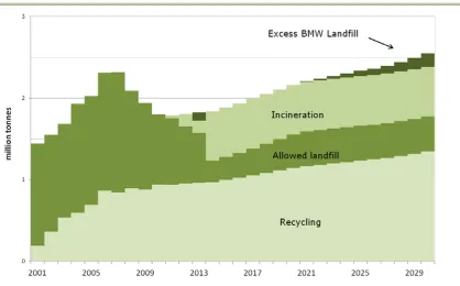
Figure 3.2: Biodegradable Municipal Waste by Destination as Observed (2001-2010) and as Projected (2010-2030)

14 |Environment Review 2012

development and utilisation of treatment capacity (e.g. composting, rendering, etc.). The projection that there will be ‘excess BMW landfill’ is based on an implicit assumption that insufficient recycling/recovery will take place (based on current trends), whereas we make no assumption about the development and utilisation of treatment capacity by the waste management sector. The EPA’s pre-treatment guidelines for landfill (EPA, 2009) implicitly assume the opposite, that is, that waste operators will develop sufficient treatment capacity and outlets for BMW. Our projections should not be interpreted as a forecast of future compliance with the Landfill Directive but instead they highlight that, with the expected growth in population and associated waste generation, and allowing for improved recycling rates, compliance with the Landfill Directive’s targets will be an ongoing challenge for the waste management sector. Our figures suggest that, while pre-collection activity (e.g. segregating waste for recycling) is important, increasingly greater capacity will be needed in post-collection treatment of the residual waste bin.

3.3.1 Sensitivity Analysis of Waste Parameters

Waste projections in the ISus model are based upon a range of assumptions about an uncertain macroeconomic environment. There are also assumptions about the micro-economic behaviour of households and businesses with respect to the generation of waste and decisions on its management. Some of the parameters of the waste model are taken from Irish research and, where that is not available, we use international research findings. But for some model parameters we have no existing research for guidance. Undertaking sensitivity analysis demonstrates the uncertainty inherent in the model, as well as identifying where new research could be most beneficially targeted. In this section we report on a sensitivity analysis of parameters related to waste in the industrial, commercial and residential sectors.

Environment | 15

in average household size. To investigate the sensitivity of MSW and BMW projections to the value of this parameter we ran scenarios with the elasticity at values of 0.65 and 0.85. In the case of the parameter increasing to 0.65 the change in MSW and BMW projections are always within 5 per cent of the original projection, as shown in Figure 3.3. When the projections are based on an elasticity value of 0.85 the new projections are within 5 per cent of the baseline projections until 2023 and greater thereafter. On a practical level the difference in projected tonnage of BMW in 2020 using the current elasticity value (i.e. 0.514) versus a value of 0.85 is less than 35,000 tonnes. Given the low change in MSW/BMW generation projections, both in percentage and absolute terms, parameter uncertainty in this instance is not of significant concern.

Figure 3.3: Municipal Solid Waste (MSW) arisings as observed and projected for the baseline model (elasticity of waste per household with respect to the number of persons per household = 0.514) and scenario projection (elasticity = 0.65)

16 |Environment Review 2012

is obviously higher but in terms of total MSW projections the effect of an elasticity value set between 0.75 and 1.3 is insignificant in terms of the aggregate projection. Figure 3.4 shows the difference in MSW projections compared to a baseline elasticity assumption equal to unity, which in all instances is less than 5 per cent of total baseline projected MSW. Devitt et al. (2010) also reviewed the value of this elasticity within the model and concluded that assumptions about economic growth are more important than parameter uncertainty in this instance.

Figure 3.4: Municipal Solid Waste (MSW) arisings as observed and projected for the baseline (elasticity of waste generated per household with respect to real personal disposable income per capita = 1.0) and two scenarios (elasticity = 0.75, 1.3)

Environment | 17

for commercial BMW) are increasingly uncertain and subject to a substantial margin of error. Research on the value of this parameter would improve the reliability of waste projections from the commercial sector.

Figure 3.5: Commercial BMW arisings as observed and projected for the baseline (elasticity of commercial BMW with respect to real output = 1.0) and two scenarios (elasticity = 0.8, 1.2)

Figure 3.6: Commercial non-BMW arisings as observed and projected for the baseline (elasticity of commercial non-BMW with respect to real output = 1.0) and two scenarios (elasticity = 0.8, 1.2)

18 |Environment Review 2012

supporting evidence. We have investigated the effect of this assumption on waste projections if the true elasticity value were 0.8 or 0.9. The results are presented in Figure 3.7. If the real elasticity value is 0.9 we are overestimating industrial waste by 3 per cent in 2020 and by 5 per cent by 2030, and more than double that if the true elasticity is 0.8. If the actual (unknown) value for the elasticity is 0.9 our projection errors are relatively small but even so in 2020 represents up to 0.5 million tonnes of waste. Therefore, while the projections provide a rough baseline for industrial waste generation, from the perspective of waste management planning the projections are subject to considerable uncertainty.

Figure 3.7: Industrial Waste arisings as observed and projected for the baseline (Industrial waste elasticity with respect to turnover = 1.0) and two scenarios (elasticity = 0.8, 0.9)

Environment | 19

scenarios assuming that the diversion of BMW from residual waste declines somewhat from historical experience. McCoole et al. (2011, Table F6) report EPA approved factors to calculate the BMW content of municipal waste streams as 0.63 in 2-bin residual household waste and 0.47 in 3-bin residual household waste. We ran scenario projections where the latter parameter equals 0.52 and 0.58 on the assumption that enthusiasm for 3-bin collection may not be as positive as elsewhere to date and that the BMW in the residual bin does fall as much. For demonstration we follow EPA (2009) on the timeframe for the roll-out of 3-bin service to all urban areas by 2013, though we believe this to be overly optimistic. Our scenarios are presented in Figure 3.8. If the BMW factor remains at the historic level (i.e. 0.47) an additional 50,000 tonnes of BMW will be recycled by 2013 and increasing thereafter as waste generation trends upwards. If the BMW factor in the 3-bin residual stream is just 5 percentage points higher (i.e. 0.52) the level of recycling falls by roughly 16,000 tonnes in 2013 compared to the 0.47 baseline. A further fall of 20,000 tonnes if the BMW factor is 0.58. While the focus of policy with respect to 3-bin collection is largely the expansion of service, the analysis here shows that equally critical to the success of the policy is the extent to which BMW material is actually diverted from the residual bin in households with 3-bin service.

20 |Environment Review 2012

3.4 A

Emissions projections from the agricultural sector are based on a projection of agricultural activity Teagasc (Donnellan and Hanrahan, 2011). Teagasc’s projection covers the period to 2020. We assume no change in the

composition of land-use or livestock numbers beyond 2020. The ISus

baseline projections reported above use Teagasc’s ‘no policy change’ baseline scenario, which excludes implementation of the Food Harvest 2020 strategy. Under the ‘no policy change’ baseline agricultural income is projected to grow substantially, due largely to increased dairy sector output following the abolition of the milk quota in 2015. Greenhouse gas emissions, under the ‘no policy change’ scenario decline until 2015 and rise marginally thereafter, which is mainly due to underlying assumptions that beef cow numbers decline as dairy cows increase and no marked increase in fertiliser use. If suckler cow numbers remain at near current levels, as well as the dairy sector expanding, greenhouse gas emissions will be higher.

Food Harvest 2020 is the strategy for the development of the agri-food and fisheries sectors. Among the strategy’s proposed targets is a 50 per cent increase in milk production by 2020 (compared to a 2007-09 baseline). Implementation of this target will have an impact on environmental emissions, in particular greenhouse gas emissions. On the basis of Teagasc’s ‘no policy change’ scenario, livestock related greenhouse gas (GHG) emissions from the agricultural sector will be roughly 16.5-16.75 million tonnes during 2015-2020.13 _{With implementation of the Food Harvest 2020}

strategy GHG emissions are projected to be 1 million tonnes higher. Under the EU Commission’s proposals outlined in the EU 20-20-20 strategy, Ireland is required to deliver a 20 per cent reduction in non-ETS GHG emissions by 2020 (relative to 2005 levels). In 2010, the agriculture sector accounted for over 42 per cent of non-ETS emissions (EPA, 2010) and consequently it is likely that the sector will have to play an important role in achieving the EU target. Reducing its GHG emissions and achieving Food Harvest 2020 targets will be a major challenge for the sector.

An expansion in the national herd will also increase the volume of manure that must be managed. An additional 22,000 tonnes of excreted nitrogen in 2020 is projected compared to the baseline, as shown in Figure 3.9.14 _In

many places surface and ground waters already have high levels of nutrient

13 _{This excludes fuel related GHG emissions.}

Environment | 21

enrichment and it is difficult to envisage how this problem will not be exacerbated with the implementation of the strategy.

Figure 3.9: Agriculture Greenhouse Gas (GHG) Emissions (excluding emissions from fuel) and Nitrogen excretion projections under baseline and Food Harvest 2020 scenarios

Since the last Environmental Review we have decomposed national

agricultural emissions into regional estimates using the census district electoral division (DED) areas as the basic geographical unit.15 _Spatially

representing the emissions estimates enables us to combine across agricultural enterprises (e.g. beef, sheep, arable) and identify from which areas the highest levels of emissions originate. For example, Figure 3.10 shows estimates of 2009 GHG emissions from cattle and sheep by DED. This type of spatial analysis of emissions enables us to examine the relationship between agricultural (and other) emissions and environmental quality (e.g. water quality). This will be the focus of future research. The spatial emissions estimates in Figure 3.10 use data from the CSO’s 1990 Census of Agriculture, as well as more periodic surveys on land use and animal populations. Initial reports from the 2010 Census of Agriculture have been published and when the detailed results are published at the end of 2012 these regional agricultural emissions will be updated.

22 |Environment Review 2012

Discussion and Conclusion | 23

Chapter 4

Discussion and Conclusion

The Environment Review 2012 covers a range of topics from greenhouse gas emissions, agriculture and waste, past trends and future projections. The full set of ISus model projections is even broader.16 _{The topics highlighted}

here are of particular interest to current policymaking.

Compliance with Greenhouse Gas Emissions Targets: Because of the severe recession, aggregate national greenhouse gas emissions are likely to be within national targets under the Kyoto Protocol though emissions from non-ETS sources will still exceed their allocated share. Prospects for compliance with longer term targets are less benign. While current climate policies have been effective at reducing the growth rate of emissions, they are insufficient to reduce the absolute level of emissions towards future policy targets. Growth in greenhouse gas emissions (ETS and non-ETS combined) is anticipated to be 1.4 per cent per annum in the latter half of this decade at the same time that policy targets require a reduction in emissions. Meeting the EU 20-20-20 target for non-ETS emissions is a massive challenge: a 20 per cent reduction in non-ETS emissions by 2020 compared to 2005. We project a growth in non-ETS emissions of 5 per cent (excluding emissions growth from the agri-food sectors associated with the Food Harvest 2020 strategy).17 _{Our analysis also suggests that}

implementation of the Food Harvest 2020 strategy could result in an additional 1 million tonnes of CO2 eq emissions from livestock, (as well as

additional emissions from the food processing sector). To comply with emissions targets significant structural change is required, whether it is in renewable energy, transport, residential fuel, or agriculture.

Food Harvest 2020: Agriculture accounts for 18.7 million tonnes of

greenhouse gas emissions ( CO2 equivalent) or 30 per cent of national total,

the highest sector share. Emissions from the sector have declined by 2 million tonnes over the past decade but full implementation of Food Harvest 2020 will reverse that trend. A starting point for a policy on meeting the EU

16 _{Further details on the projections are available at esri.ie/research/research_areas/environment/isus/}

17 _{This contrasts with EPA (2012), which projects a decline in non-ETS emissions but is based on alternative}

24 |Environment Review 2012

20-20-20 target should be no increase in emissions from the sector. An estimated additional 1 million tonnes of GHG emissions associated with implementation of Food Harvest 2020 means that a balancing reduction in emissions will have to be achieved elsewhere in the economy. There is an argument that the burden of additional emissions from agriculture should be borne by the sector itself and the sector’s development strategy should be revisited to examine how this should be achieved. However, agriculture is a special case in that if climate policies curtail Irish milk and beef production, production will move overseas to places like Brazil without any global environmental benefit. Preserving emissions efficient production within Europe would be preferable. Consideration should therefore be given to seeking, at EU level, a special mechanism for managing agricultural emissions within Europe. Ireland has a comparative advantage in beef and dairy production and has the potential to expand output and employment; however, the current mechanism for managing emissions within the sector is a threat to realising those benefits.

Emissions Trading System: The EU-ETS will play its role in reducing emissions but while it regulates large emitting installations it excludes a significant share of total emissions (e.g. agriculture, much of transport and residential). The carbon tax, which applies to the rest of the economy, will also curtail emissions growth but will be insufficient to achieve the dramatic emissions reductions necessary to reach policy targets (FitzGerald et al., 2008, p117).18 _{Within energy, fuel switching offers some scope for emissions}

reduction. In 2010 peat accounted for 5.4 per cent of the total primary energy requirement of the state and 10 per cent of the electricity generation fuel mix, yet it contributes more than double the amount of CO2

emissions per unit energy compared to gas and 59 per cent higher than oil (SEAI, 2011). The phase out of peat in electricity generation (which is already declining) would make a contribution to emissions reduction without significant negative impact on competitiveness, though it would not contribute to achieving the non-ETS emissions targets. Extending the carbon tax to peat would discourage its use in the residential sector (e.g. peat briquettes) and make a small contribution to emissions reduction. However, a significant benefit of the phase out of peat as a fuel would be a reduction in particulate emissions, which have an adverse impact on health. 19

18 _{Under the scenario presented it is assumed that the carbon tax will increase from €20 in 2011 reaching €32 by}

2020 and €47 by 2030 matching the projected price of allowances in the EU-ETS and applies to all fuels including peat and coal. Peat and coal are currently not subject to the carbon tax.

19 _{The Department of the Environment, Community and Local Government’s recent public consultation document,}

Discussion and Conclusion | 25

Renewables: The other obvious area to reduce emissions from the energy sector is an expansion of the share of energy from renewable sources. While this has potential environmental benefits, the failure of the sector to expand,20 _{particularly in biomass energy, is reflective of a difficult business}

proposition as well as technical challenges.21 _{Biomass is problematic as it}

produces significant amounts of particulate matter, which can have serious health impacts. Current schemes for feed-in tariffs for renewable energy projects (i.e. REFIT 2 and REFIT 322_{) will support renewable energy but}

beyond that the outlook for expansion will remain difficult given business, planning, financial and technological challenges. To achieve a dramatic increase in renewable energy a wider review of renewable policy at EU level and its impact on competitiveness and environmental benefits is merited (FitzGerald, 2011).

Water Quality: Nutrient enrichment of surface and ground waters is prevalent in many locations and agriculture is one of the contributory sources.23 _{With increased volumes of excreted nutrients associated with}

growth in the sector, Food Harvest 2020 has the potential to exacerbate the problem. As instances of poor water quality occur with current levels of output, it is difficult to argue that existing nutrient management practices are adequate to protect the environment from further harm (or return water quality to a ‘good’ status as required under the Water Framework Directive). Protecting water quality from diffuse pollution24 _{sources is}

extremely difficult and the onus should be on all sources (i.e. municipal, agriculture, residential) to demonstrate that their activities are not causing environmental damage. The establishment of a system to verify implementation of best practice for nutrient management would assist expansion in the sector while protecting environmental quality.

Industrial Sector: Projections of F-gases, largely from the industrial sector, will account for an increasing share of greenhouse emissions in the future with the potential to increase from 1 to 4 per cent share within a decade. This projection is subject to a considerable margin of error, as the ISus

20 _{Renewables accounted for 4.6 per cent of total primary energy requirement in 2010 (SEAI, 2011).}

21 _{In addition to technical issues associated with renewable technologies, the expansion of the share of energy}

from renewable sources will also be dependent on interconnection capacity to the UK to manage supply imbalances.

22 _{See www.dcenr.gov.ie/Energy/Sustainable+and+Renewable+Energy+Division/REFIT.htm}

23 _{Discharges from urban waste water treatment plants and septic tank outflows are among the other major}

contributory sources.

24 _{Nutrients are a resource when recycled within the assimilative capacity of the land but become pollutants when}

26 |Environment Review 2012

model does not have detailed information on the emission sources. However, the projection does highlight that this type of emission source could be quite significant in the future. The current review of the European regulation on F-gas emissions is an opportunity to amend current controls to ensure that the growth in F-gas emissions will not offset emissions reductions achieved in other areas.

Appendix 1: The ESRI Environmental Accounts | 27

Appendix 1: The ESRI Environmental Accounts

The national accounting framework, including such key concepts as Gross National Product, is a vital input to economic decision making. However, the standard national accounting framework does not take account of the pressure or damage to the environment caused by the economic activity. Thus, similar levels of GNP might involve quite different environmental damage, with implications for both current and future welfare and economic activity. Environmental accounts are now constructed in many countries to take account of these concerns, building on initial research by Nordhaus et al. (1972) and agreed international standards (United Nations et al. 2003). Environmental accounts build on the well-established and coherent national accounting framework, but add to this with what are termed “satellite accounts” dealing with environmental issues, in a way which allows for them to be integrated and measured in a more comprehensive framework. This provides an increasingly sound basis for decision making on the environment.

Lyons et al. (2009) present the ESRI Environmental Accounts for the Republic of Ireland 1990-2006. The paper describes the principles of environmental accounts, and illustrates their use by discussing trends in emissions and resource use in Ireland, by comparing the trend in carbon dioxide emissions in Ireland to other countries, and by attributing emissions to consumption.

28 |Environment Review 2012

The ESRI Environmental Accounts are proper satellite accounts of the National Accounts. We can therefore readily integrate economic and environmental data. This allows us to interpret trends and, for example, allocate responsibility for particular emissions to the relevant sectors of activity.

Revised Structure of Waste Accounts

Version 0.7 of ISus fully implements the bio-waste category that was introduced in the previous version of the ESRI Environmental Accounts. We now have a potential 25 waste categories (5x5), which are made up of five dispositions (landfilled, recycled, incinerated, used as fuel and unattributed) for five substances (hazardous, bio-waste, BMW biowaste, other non-biowaste and soil & stones). We have one secondary material, incinerator ash, that as of now has a disposition of unattributed. Not all combinations of waste type and dispositions are operative due to the nature of the material. In the matrix below an “X” denotes combinations that are present in our accounts:

Primary

Materials Secondary Materials

Dispositions Hazardous Bio-Waste BMW,

non-Biowaste Other, non-Biowaste Stones Soil & Incinerator Ash (organic) (non-organic)

Landfilled X X X X X Recycled X X X X X Incinerated X X X X

Used as fuel X X X

Unattributed X X X X X X

In addition, the ISus model reports summary waste emission categories that are of policy interest: biodegradable municipal waste (BMW), municipal solid waste (MSW), construction and demolition (C&D), and industrial waste. These totals are calculated by selecting relevant sectors and materials from the basic set of accounts.

Appendix 1: The ESRI Environmental Accounts | 29

Content of New Waste Categories

Bio-waste

The bio-waste emission category was introduced in the 2008 Waste Framework Directive,25 _{which defined it as “biodegradable garden and park}

waste, food and kitchen waste from households, restaurants, caterers and retail premises and comparable waste from food processing plants.” Bio-waste includes the organic fraction of biodegradable municipal Bio-waste (BMW). All bio-waste is not BMW and not all BMW is bio-waste. We estimate biowaste as the sum of the organic component of BMW and the component of industrial waste tagged with the European Waste Catalogue (EWC) codes or EWC-STAT codes listed in Table A.1 below. The main sectoral sources are households, commercial enterprises and the food processing sector.

Table A.1: EWC and EWC-STAT Codes Used to Identify Bio-Waste

EWC code Description

02 02 01 sludges from washing and cleaning 02 02 02 animal-tissue waste

02 02 03 materials unsuitable for consumption or processing

02 03 01 sludges from washing, cleaning, peeling, centrifuging and separation 02 03 02 wastes from preserving agents

02 03 04 materials unsuitable for consumption or processing 02 05 01 materials unsuitable for consumption or processing 02 06 01 materials unsuitable for consumption or processing 20 01 08 biodegradable kitchen and canteen waste

20 01 08 01

20 01 25 edible oil and fat 20 01 25 01

20 01 25 03

20 02 01 biodegradable waste

EWC-STAT code Description

9 Animal and vegetal wastes

9.11 Animal waste of food preparation and products 9.12 Vegetal waste of food preparation and products 9.13 Mixed waste of food preparation and products 9.2 Green wastes

9.21 Green wastes

25 _{Directive 2008/98/EC of the European Parliament and of the Council, on waste and repealing certain Directives,}

30 |Environment Review 2012

BMW, non-biowaste

Earlier versions of the Environmental Accounts contained a separate waste category for biodegradable municipal waste (BMW). As bio-waste, the new regulatory waste classification mentioned above, partially overlaps BMW we have reorganised the accounts to account for both bio-waste and BMW. The “BMW, non-biowaste” category is essentially the non-organic fraction on BMW. The organic fraction of BMW is included in “bio-waste”. Total BMW can be easily retrieved by summing the relevant sectors from these two categories.

Other, non-biowaste

This waste category comprises materials that are non-hazardous, non-BMW, and non-biowaste.

Used as fuel

This disposition is currently attributed only to industrial sectors. It is used for waste flows that are tagged with D/R code “R1” by the EPA (see EPA (2012) for further details of disposal and recovery coding). There is a regulatory distinction between this form of treatment and incineration, which is tagged with code D10.

Soil and stones (non-hazardous component)

This material, attributed to the construction sector, is separately identified in EPA National Waste Reports so we have given it a separate accounting category. It should be added to “Other, non-biowaste” and “Hazardous” waste emissions from the construction sector to arrive at total C&D waste.

Incinerator bottom ash

We describe this as a secondary material, because it results from material already counted as incinerated. Incinerator ash should not simply be added to other emission categories, because this could lead to double-counting of some material in mass-balance terms.

Base Year Values

Appendix 1: The ESRI Environmental Accounts | 31

we report are constituted, making reference to (McCoole et al., 2010, 2011 and 2012), which we refer to as NWR08, NWR09 and NWR10.

Hazardous waste

We include both contaminated soil and other hazardous waste; the total given is equal to the sum of the totals in NWR10 Tables 27 and 35.

MSW

This category in our model only approximately equates to the regulatory category of the same name. To the MSW figure in Table 2 of NWR10 we add estimated uncollected household waste (section 3.3.4, NWR10) and sewage sludge (for which the data relates to 2007 and which we treat as largely attributable to the household and commercial sectors).

C&D and Industrial

Appendix 2: Ireland’s Sustainable Development Model (ISus) | 33

Appendix 2: Ireland’s Sustainable Development Model

(

ISus

)

ISus is a simulation model. It combines behavioural equations and data on state variables in period t to predict the state variables at time t+1. The current version of the model (v0.7) mostly uses data for the period 1990-2009 (the period covered by the ESRI Environmental Accounts) to calibrate the model and estimate relationships, while projections are generated for

the period 2010-2030 (the period covered by HERMES, ESRI’s

macroeconomic model). In the case of most waste streams the model uses data up to 2010 and projections cover the period 2011-2030.

Figure A2.1 shows the relationship between ISus and other models. Two models are used for the international context: NiGEM (NIESR’s global macroeconomic model), and HTM (Hamburb Tourism Model). NiGEM is used for scenarios on the overall macroeconomic situation, while HTM

zooms in on tourism. The ICPop model generates scenarios of the

population of Ireland and its structure. The HERMES model takes output from NiGEM and HTM as given, and it interacts with IDEM (an electricity

34 |Environment Review 2012

generation model) and ICPop (on migration) to build scenarios of the macroeconomy of Ireland. IDEM takes world energy prices from NiGEM and the demand for electricity from HERMES to generate scenarios of power supply; IDEM and HERMES iterate on electricity supply. ISus takes population from ICPop, energy use in the electricity sector from IDEM and macroeconomic variables from HERMES.

Figure A2.2 shows the internal structure of ISus. The model is split between consumption and production, and production is split into power generation, other energy, transport, agriculture and other production. These six inputs are used to generate resource use, emissions, and waste from 20 sectors. An input-output model is then used to attribute emissions etc. from production to the components of final demand.

Further documentation and the model code can be found at: http://www.esri.ie/research/research_areas/environment/ISus/

Figure A2.2: Flowchart of ISus

A2.1 Agricultural Activity

Appendix 2: Ireland’s Sustainable Development Model (ISus) | 35

model uses these inputs to project emissions to 2030 following EPA’s methodology for calculating emissions from agriculture. In the scenarios presented earlier we utilise Teagasc’s FAPRI (Food and Agricultural Policy Research Institute) model’s livestock and land use projections as exogenous inputs into the agriculture sub-model. FAPRI uses ESRI’s HERMES model for its macroeconomic projections so there is a consistency in the underlying macroeconomic assumptions.

A2.2 Energy Use and Related Emissions

The energy use model was developed in a previous ESRI project for the EPA. The equations have not changed, but the model was re-estimated using more recent data. Emissions follow by multiplying energy use with the appropriate emission coefficients. The full model description can be found in Fitz Gerald et al. (2002).

A2.3 Waste Arisings and Disposition

The waste sub-models project future volumes based on output, income, other behavioural drivers and some supply effects, together with elasticity assumptions. The full model description can be found in Devitt et al. (2010).

A2.4 Methane from Landfill

We impute historical amounts of landfilled waste in the Republic of Ireland so as to estimate methane emissions. The model distinguishes between waste from households and from small businesses and we model waste arisings as a function of the size of the service sector, the size of the population, per capita income, and the price of disposal. The full model description can be found in Devitt et al. (2010).

A2.5 Emissions from Other Production

There are four ways to project emissions from and resource use by economic production within ISus:

1. Output elasticities. 2. Intensity trends.