Small Area Estimation under a Two Part Random Effects Model with Application to Estimation of Literacy in Developing Countries

SMALL AREA ESTIMATION UNDER A TWO PART RANDOM EFFECTS

MODEL WITH APPLICATION TO ESTIMATION OF LITERACY IN

DEVELOPING COUNTRIES

DANNY PFEFFERMANN, BÉNÉDICTE TERRYN, FERNANDO MOURA

ABSTRACT

The UNESCO Institute for Statistics has initiated a programme to collect data on the level of literacy of adults in developing countries. This will involve conducting small-scale surveys in a few countries that will consist of giving interviewees aged 15+ a test to measure their literacy score. One of the main objectives of these surveys is to obtain summary measures of literacy levels in small geographical areas for which only very small samples would be available, thus requiring the use of model based small area estimation methods.

Available methods are not suitable, however, for this kind of data due to the mixed distribution of the literacy scores in developing countries. This distribution has a large peak at zero, i.e., a large proportion of adults that are illiterate, and juxtaposed to this peak is an approximately bell-shaped distribution of the non-zero scores measured for the rest of the sample.

In this paper we develop a two part three-level model that is suitable for this kind of data and show how to obtain the small area measures and their variances, or compute confidence intervals, based on this model. The proposed method is illustrated using simulated data and data obtained from a similar literacy survey conducted in Cambodia.

Compilation © 2005 Association for Survey Computing

Small Area Estimation under a Two-Part Random Effects Model

with Application to Estimation of Literacy in Developing Countries

Danny Pfeffermann, Bénédicte Terryn, Fernando Moura

Abstract

The UNESCO Institute for Statistics has initiated a programme to collect data on the literacy skills of adults in developing countries. This involves conducting small-scale surveys in a few countries, which consist of administering interviewees aged 15+ a test to measure their literacy score. One objective of this programme is to obtain summary measures of literacy levels in geographical areas for which only very small samples would be available, thus requiring the use of model based small area estimation methods.

Available methods are not suitable, however, for this kind of data due to the mixed distribution of the literacy scores in developing countries. This distribution has a large peak at zero, i.e., a large proportion of adults that are illiterate, and juxtaposed to this peak is an approximately bell-shaped distribution of the non-zero scores measured for the rest of the sample.

In this presentation we will develop a two-part three-level model that is suitable for this kind of data and show how to obtain the small area measures and their variances, or compute confidence intervals, based on this model. The proposed method will be illustrated using simulated data and data obtained from a literacy survey conducted in Cambodia.

Keywords

MCMC,generalized linear mixed model, linear mixed model

1 Introduction

We consider the distribution of scores obtained from literacy tests administered to adults in a household survey. In most developing countries, where many people cannot read or write, this is not a standard distribution. Typically, it consists of a large peak at zero, juxtaposed to a continuous distribution for the non-zero scores, as observed, for example, in a literacy survey carried out in Cambodia in 1999 (see Figure 1 below).

covariates. The model accounts for correlations between the corresponding random effects of the two parts. The model is fitted by application of Markov Chain Monte Carlo (MCMC) simulations.

[image:3.595.151.416.257.413.2]

The two-part model is applied to data collected as part of a national literacy household survey carried out in Cambodia in 1999, known as the ‘Assessment of the Functional Literacy Levels of the Adult Population’. The performance of the proposed model is tested by simulating data sets that mimic the Cambodia data. The use of simulations also enables us to compare the results of fitting the full model with the results obtained when fitting the two parts of the model separately, without accounting for the correlations between the random effects in the two parts. Another comparison of interest is to results obtained when ignoring the special nature of the data and fitting the linear part to the whole data, ignoring the problem of many zero scores.

Figure 1. Histogram of literacy scores in a national literacy survey in Cambodia, 1999

0 500 1000 1500 2000 2500 3000

2.5 17.5 32.5 47.5 62.5 77.5 92.5

2 Model and small area predictors

Let Ydefine the response value (literacy test score in our application) and R the covariate variables and random effects. Then,

( | , 0) Pr( 0 | )

E Y R r Y Y R r

+ = > > =

=

E Y R r Y

( |

=

,

>

0)Pr(

Y

>

0|

R r

=

)

(1)

since

E Y R r Y

( |

=

,

= =

0) 0

. For the small area estimation application considered in this paper we consider a nested 3 level model with districts of residence defining the first level, villages defining the second level and individuals defining the third level. For individual k residing in village j of district

i

, we have therefore the relationship,

(

_ijk

|

_ijk

)

(

_ijk

|

_ijk

,

_ijk

0)Pr(

_ijk

0|

_ijk

)

E y

r

= =

r

E y

r

=

r y

>

y

>

r

=

r

(2)

In what follows we model the two parts in the right hand side of (2). For individuals with positive responses we assume the familiar ‘linear mixed model’,

| ,

0

'

ijk ijk ijk ijk i ij ijk

y

r y

> =

x

β

+ + +

u v

ε

;

u

_i

~ (0,

N

σ

_u2

) ;

v

_ij

~ (0,

N

σ

_v2

) ;

ε

_ijk

~ (0,

N

σ

_ε2

)

(3)

where x_ijk represents individual and area level values of the covariates, u_i is a random district effect and v_ij is a nested random village effect. The random effects and the residual terms ε_ijk are assumed to

be mutually independent. Notice that by (3),

(

_ijk

| ,

_{ijk ijk}

0)

The random effects account for the variation of the individual responses not explained by the covariates. Alternatively, they define the correlations holding between the responses of individuals residing in the same village, or individuals residing in the same district but in different villages.

2 2 2 2 2

2 2 2 2

' ' '

( )/( ) if ', '

( , ) /( ) if ', '

0 if '

u v u v

ijk i j k u u v

j j k k

Corr Y Y i i j j

i i ε

ε

σ σ

σ σ σ

σ σ σ σ

⎧ + + + = ≠ ⎪ =⎨ + + = ≠ ⎪ _≠ ⎩ (4)

For the probabilities of positive responses (second part of (2)) we assume the ‘generalized linear mixed model’,

* * * *

* *

exp ( '

)

Pr (

0| , , )

1 exp ( '

)

ijk i ij

ijk ijk i ij ijk

ijk i ij

x

u v

Y

x u v

p

x

u v

γ

γ

+ +

>

=

=

+

+ +

;

* 2 * 2

* *

~ (0,

) ;

~ (0,

)

i u ij v

u

N

σ

v

N

σ

(5)

implying,

(

) log

1

ijk ijk ijk

p

logit p

p

=

=

−

* *

'

ijk i ij

x

γ

+

u

+

v

. Here again

u

_i* and

v

_ij* represent random

district and village effects not accounted for by the covariates.

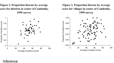
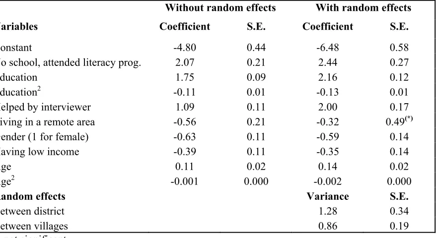
The proposed model permits nonzero correlations between the district random effects in the two parts, and similarly for the village random effects. This is a reasonable assumption since it can be expected that for given values of the covariates, an individual residing in an area characterized by high literacy scores will have a higher probability of a positive score than an individual residing in an area with low scores. See Figures 2 and 3 below for some supporting evidence from data in Cambodia. (The correlations are 0.35 for villages and 0.38 for districts.) The correlations are modelled by assuming,

*

* 2

|

| ~ ( , )

i i u i _{u u}

u u N K u σ ; *

* 2

|

| ~ ( , )

ij ij v ij _{v v}

v v N K v σ (6)

Let

U

_i define the population of first level

i

of size

N

_i. The small area parameters of interest are the means,

Y

_i

=

∑

_j,k∈Ui

y

_ijk

/

N

_i, which in the case of the survey in Cambodia are the true district means

of the literacy scores. Notice that the means are computed over all the individuals in the area, including individuals with zero scores. Under the model defined by (2), the means can be predicted as,

]} ˆ ) 0 , ( ˆ [ { 1 ˆ ,

,k si ijk jk si ijk ijk ijk ijk j

i

i _N y E Y r Y p

Y =

∑

_∈ +

∑

_∉ > × (7)

where

s

_i defines the sample from first level (district)

i

. By (3) and (5), the predictor in (7) takes the form,

* *

, , * *

ˆ ˆ ˆ

exp ( '

)

1

ˆ

_[

₍

_{ˆ ˆ ˆ}

₎

_]

ˆ ˆ ˆ

1 exp ( '

)

i i

ijk i ij

i j k s ijk j k s ijk i ij

i ijk i ij

x

u v

Y

y

x

u v

N

x

u v

γ

β

γ

∈ ∉

+ +

=

+

+ + ×

+

+ +

∑

∑

(8)

with ˆ ˆ ˆ ˆ ˆ ˆ_{, , , , ,}* *

i i i ij u v u v

[image:5.595.67.515.60.311.2]

Figure 2. Proportion literate by average score for districts in center of Cambodia,

1999 survey

0 0.2 0.4 0.6 0.8 1

0 20 40 60 80 100

Average of positive scores

P

ropor

tion

of

po

si

tiv

e s

cor

es

Figure 3. Proportion literate by average score for villages in center of Cambodia,

1999 survey

0.00 0.20 0.40 0.60 0.80 1.00

0 20 40 60 80 100

Average of positive scores

P

ropor

tion of

pos

iti

ve s

cor

es

3 Inference

The use of the small area predictors defined by (8) requires estimating the fixed parameters

2 2 2

( ,β σ σ σ_u, _v, ε) of the linear part (Equation 3), the fixed parameters * *

2 2

| |

( ,γ K K_u, _v,σ_{u u},σ_{v v}) of the

logistic part (Equations 5, 6), and predicting the random effects

λ

ij

=

{( , ; , )}

u v u v

i ij i* ij* . Methods for estimating the fixed and random effects when fitting linear mixed models or generalized linear mixed models alone have been developed over the last two decades under both the frequentist and the Bayesian paradigms. The use of these methods permits also the computation of estimators of the mean square error (MSE) of the small area predictors that account for parameter estimation to correct order; see the recent book of Rao (2003) for a thorough review and discussion. However, the two-part model defined by (2)-(6) has not been considered in the literature in the context of small area estimation and in what follows we describe briefly a few possibilities of fitting this model.

Likelihood based inference

Define, 1Ι =_ijk if Y_ijk >0, 0Ι =_ijk ifY_ijk =0, and denote

r

ijk

=

( , , )

x u v

ijk i ij ,

r

ijk*

=

( , , )

x u v

ijk *i *ij . For given vectors

r r

ijk

,

ijk* , the likelihood for the two-part model takes the form,

(1 )

, ,

( )ijk ( | 0) (1ijk ) ijk

ijk ijk ijk ijk

i j k s

L p Ι f y y Ι p −Ι

∈

=

∏

> − (9)

with

p

_ijk and f y( _ijk | y_ijk >0) defined by (5) and (3) respectively and

s

= ∪

s

_i denoting the sample

from all the areas. The use of this likelihood for inference is, however, problematic because the

random effects

λ

ij

=

{( , ; , )}

u v u v

i ij i* ij* are in fact unobservable random variables. One possibility,

therefore, is to integrate the likelihood over the joint (normal) distribution of the random effects as defined by (3) and (6), and maximize the integrated likelihood with respect to the fixed parameters

2 2 2

( ,

β σ σ σ

_u

,

_v

,

_ε

)

and * *

2 2

| |

(1 ) 0

, ,

( )ijk ( | 0) (1ijk ) ijk ( )

ijk ijk ijk ijk ij ij

i j k s

L p Ι f y y Ι p −Ι g λ dλ

∈

=

_∫

∏

> − . Olsen and Schafer (2001) consider a similar

two-part model for fitting longitudinal data. The authors approximate the integrated likelihood by a high order multivariate Laplace approximation (Raudenbush et al. 2000), and calculate empirical Bayes predictors of the random effects by use of importance sampling (Tanner, 1996), setting the fixed parameters at their maximum likelihood estimates. The application of this procedure, however, is complicated computationally and the MSE estimators of the small area predictors obtained this way fail to account for the variation induced by estimating the fixed parameters. The contribution of fixed parameter estimation to the total MSE can not be ignored in general, unless the number of sampled areas is large.

Separate model fitting:

The idea here is to fit the two parts of the model separately and then combine the estimates for computing the small area predictors in (8). As mentioned earlier, the fitting of the separate parts has been researched extensively in the literature over the last 2 decades and computer software is now readily available, particularly for linear mixed models. See Rao (2003) for a short review. Note that extra care should be taken when computing MSE estimators of correct order.

The use of separate model fitting has, however, the disadvantage of not lending itself to simple computations of the coefficients (K K_u, _v) (Equation 6), and it is not clear how to account for the existing correlations between the two data sets for enhancing the efficiency of the small area predictors. Notice also that by ignoring the correlations between the random effects of the two parts of the model, the estimated MSE of the small area predictors are imprecise.

Bayesian inference

The use of Bayesian methods requires specification of prior distributions for all the fixed parameters underlying the two-part model, but with the aid of Markov Chain Monte Carlo (MCMC) simulations the use of this approach permits sampling from the posterior distribution of the fixed parameters and the random effects, and hence from the posterior distribution of the small area means, given the data. Thus, the MCMC algorithm yields the whole posterior distribution of the small area means of interest, and hence correct MSE (posterior variance) estimators or confidence (credibility) intervals can be computed. Computer software is available to perform all the necessary computations but it should be noted that with complex models the computations can be very intensive and time consuming.

* *

, , * *

exp ( '

)

1

[

(

)

]

1 exp ( '

)

i i

ijk i ij

i j k s ijk j k s ijk i ij

i ijk i ij

x

u v

y

x

u v

N

x

u v

γ

θ

β

γ

∈ ∉

+ +

=

+

+ + ×

+

+ +

∑

∑

(compare with (8)). Repeating the

same sampling process independently a large number of times yields an approximation to the posterior distribution of each of the values

θ

_i. The true small area mean,

Y

_i, can then be predicted by averaging the sampled values

θ

_i in all the chains. (The average estimates the posterior expectation of the small area mean, see also the comment below.)

The MSE is estimated by computing the empirical variance of the sampled values from the posterior distribution of the means

Y

_i. The sampled values are obtained by first predicting the individual

nonsampled measurements

y

_ijk and then computing the means

]

ˆ

[

1

ˆ

, ,k s_i ijk jk s_i ijk j

i

i

y

y

N

Y

=

∑

_∈

+

∑

_∉ . The predictors

y

ˆ

_ijk are computed by randomly drawing

from their posterior distribution, i.e.,

ˆ

_ijk

(

_{ijk i ij ijk}

)

_ijk

y

=

x

β

%

+ + +

u v

_{% %}

ε

_%

×Ι

%

(10)

where, Ι =%_ijk 1 with probability

p

%

_ijk and Ι =%_ijk 0 with probability

(1

−

p

%

_ijk

)

,

* *

* *

exp ( '

)

1 exp ( '

)

ijk i ij

ijk

ijk i ij

x

u v

p

x

u v

γ

γ

+ +

=

+

+ +

% % %

%

% % %

. Notice that each of the fixed and random effects used for the prediction

of the measurements

y

_ijk (denoted by “~”) is a random draw from its posterior distribution. Confidence (credibility) intervals with coverage rates of

(1

−

α

)

are defined by the

α

/ 2 and

(1

−

α

/ 2)

level quantiles of the empirical posterior distribution of the

Y

_i(the distribution of the

sampled values

Y

ˆ

_i).

In practice, the use of parallel chains for producing independent realizations is often too time consuming, in which case the samples can be generated from a single long chain or a few chains, but selecting only every rth _{sampled value (after convergence), thus reducing as much as possible the}

dependencies existing between adjacent sampled values.

Comment: The posterior mean of

Y

_i could also be estimated by simply averaging the sampled values

ˆ

i

Y

from its posterior distribution. Notice, however, that these values contain also the sums

, _i

ˆ /

ijk i

j k s∉

ε

N

∑

for which the posterior mean is zero, so that the use of this procedure adds some extra noise to the estimation of the posterior mean if the number of MCMC simulations is not sufficiently large (depending also on the posterior variance of the

ε

_ijk).

4 Empirical

Results

the provinces half of the districts were selected, then within each district 2 communes were selected and within each commune, 3 villages were selected (with a few exceptions). Finally, households were selected in each village and one adult sampled from each household, altering according to age and sex. The sampling scheme at each stage was systematic sampling. The number of households selected in each village was constant for all the sampled villages belonging to the same province. The province total sample sizes were allocated proportionally to the population province sizes.

In what follows the small areas of interest are the country districts, with sample sizes varying between 0 (no sample) in 88 of the districts to almost 150 in the districts of the capital city. Twenty one districts had sample sizes less than 20, and another 16 districts had sample sizes between 41 and 60. The data analyzed for this study refer to the 50 rural districts in provinces located in the center of the country. The total sample size is n=4028.

Table 1 shows the results obtained when fitting the logistic model alone to this data set, with and without random effects for districts and villages. The dependent variable

Ι

_ijk takes the value 1 if

0

ijk

[image:8.595.97.536.467.707.2]

y

>

and takes the value 0 otherwise, see Equation (5). Table 2 shows the results of fitting the linear model to individuals with positive scores alone, again with and without the inclusion of random effects. These two models have been fitted using the MLwiN software (Goldstein, 2003). This software computes maximum likelihood estimators of the fixed parameters and empirical best linear unbiased predictors (EBLUP) of the random effects for linear mixed models, and predictive quasi likelihood estimators (PQL) of the fixed parameters and random effects for generalized linear mixed models. (Other estimation procedures are also available.) The regressor variables in the two models have been chosen by application of some standard model selection procedures, without the inclusion of the random effects. All the variables except those referring to age, education and household size are dummy variables taking the value 1 when the variable definition is satisfied.

Table 1. Model parameters and standard errors (S.E.) when fitting logistic part alone

Without random effects With random effects

Variables Coefficient S.E. Coefficient S.E.

Constant -4.80 0.44 -6.48 0.58

No school, attended literacy prog. 2.07 0.21 2.44 0.27

Education 1.75 0.09 2.16 0.12

Education2 _{-0.11 0.01 -0.13 0.01}

Helped by interviewer 1.09 0.11 2.00 0.17

Living in a remote area -0.56 0.21 -0.32 0.49(*)

Gender (1 for female) -0.63 0.11 -0.59 0.14

Having low income -0.39 0.11 -0.35 0.14

Age 0.11 0.02 0.14 0.02

Age2 _{-0.001 0.000 -0.002 0.000}

Random effects Variance S.E.

Between district 1.28 0.34

Between villages 0.86 0.19

[image:9.595.60.497.96.339.2]

Table 2. Model parameters and standard errors (S.E.) when fitting linear part alone

Without random effects With random effects

Variables Coefficient S.E. Coefficient S.E.

Constant 5.85 4.18 6.90 4.00

Civil servant and professional 10.71 2.14 13.91 1.89

Education 6.64 0.59 7.28 0.53

Education2 _{-0.19 0.05 -0.24 0.05}

Low income -3.15 0.94 -2.61 0.88

Gender (1 for female) -2.52 0.92 -1.60 0.81

Number of adults in household 1.23 0.31 0.94 0.29

Age 1.04 0.18 0.84 0.16

Age2 _{-0.013 0.002 -0.010 0.002}

Random effects Variance S.E.

Between district 66.31 16.72

Between villages 66.58 10.45

Individual level 322.03 10.12

The main results emerging from the two tables can be summarized as follows: inclusion of the random effects in the two models changes the values of the coefficients, more so in the linear part, but not to the extent of changing their signs. The variances of the random effects when included in the model are highly significant, indicating their contribution to explaining the variation of the scores. Finally, we note the interesting outcome that in the logistic case the standard errors of the estimated coefficients when including the random effects in the model are always larger or equal than the corresponding standard errors when fitting the model without them, and that it is the other way around in the linear case. We don’t have a clear explanation to this outcome.

[image:10.595.91.534.70.280.2]

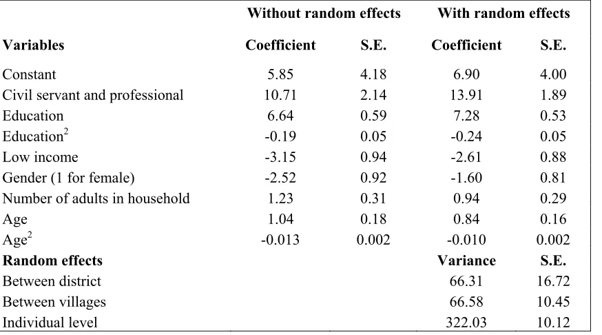
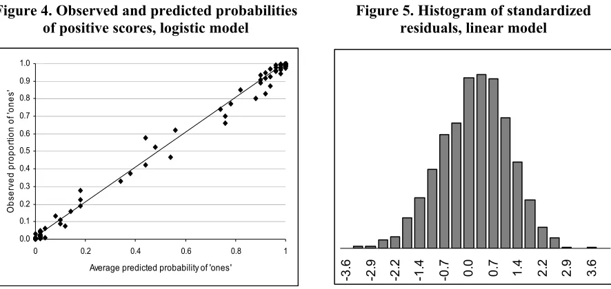
Figure 4. Observed and predicted probabilities of positive scores, logistic model

0.0 0.1 0.2 0.3 0.4 0.5 0.6 0.7 0.8 0.9 1.0

0 0.2 0.4 0.6 0.8 1

Average predicted probability of 'ones'

O

b

se

rv

ed p

ro

por

tion

o

f '

o

n

e

s'

Figure 5. Histogram of standardized residuals, linear model

-3

.6

-2

.9

-2

.2

-1

.4

-0

.7 _0.0 _0.7 _1.4 _2.2 _2.9 _3.6

5 Simulation

Study

The purpose of the simulation experiment is to study the effectiveness of the two-part model for producing small area predictors and measures of the associated prediction errors, and to compare the results with results obtained when fitting the two parts of the model separately ignoring the correlations between the corresponding random effects in the two parts, and with the results obtained when fitting a linear mixed model to the whole sample ignoring the accumulation of zero scores. To this end, we generated 300 populations of size 4,028 (the same size as the original data set analyzed in Section 4), and 300 corresponding samples of size 750, using a two-part model but with fewer regressors than in Tables 1 and 2. In the logistic part we included 4 regressors: ‘number of years at school’, ‘attendance of a literacy programme’, ‘helped by the interviewer’ and ‘having low income’. In the linear part we included 5 regressors: ‘number of years at school’, ‘gender’, ‘number of adults in the household’, ‘age’, and ‘age2_{’. In order to specify sampled values of the regressor variables, we}

sampled at random 750 individuals from the data set considered in Section 4, and the observed regressor values were then used for all the 300 samples. New random effects and errors were generated for every simulation using the model defined by (3) and (6), and added to the fixed effects

'

ijk

x

γ

and

x

_ijk

'

β

in the logistic and the linear parts for every sampled and nonsampled population unit. The correlations between the random effects of the logistic and the linear parts were set to 0.26 for the district random effects and 0.41 for the village random effects. See Table 3 for the other parameter values used for generating the data. Individual scores

y

_ijk were generated by performing Bernoulli trials with probabilities

Pr(

Ι = =

_ijk

1)

p

_ijk as defined by the logistic model in (5), and in the case of a ‘one’, generating a score from the model (3). The district means of the

y

-values in the population (zero and nonzero scores) were taken as the true district means. The samples contained individuals from all the 50 districts, with 11 districts having samples of size

1

≤

n

_d

≤

10

, 29 districts having samples of size

11

≤

n

_d

≤

20

, and the remaining 10 districts having samples of size

coefficients

β γ

,

, and uniform priors for the standard deviations underlying the two parts of the model and the coefficients

K

_u and

K

_v (Equation 6).

We encountered unexpectedly severe computation problems when fitting the two-part model with WinBUGS, accounting for both district random effects and village random effects. The sampled values generated by the Gibbs sampler were found to be strongly correlated even at very high lags, (over 1000 for the village random effects and the correlation between the village random effects in the two parts, and still over 500 when tightening the prior distributions), which required extremely long chains to obtain sufficient data for inference. We also couldn’t verify convergence of some of the posterior distributions. This made it impossible to perform a full scale simulation study and we therefore fitted the two-part model with only district level effects, despite generating the data with village random effects as well. (The predictors of the linear part remain unbiased even when ignoring the village effects. This is not true for the logistic part but the bias is small.) We are presently investigating ways of overcoming these computational difficulties. For fitting the models with the district random effects we generated chains of length 20,000, discarded the first 10,000 sampled values as “burn in”, and then thinned the chains by taking every 20th _{sample. This resulted in having}

500 sampled values from the posterior distribution of each of the fixed and random parameter values and hence 500 sampled values from the posterior distribution of each of the district means.

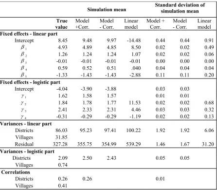
The results of the simulation study are shown in Table 3 and Figures 4-6. Table 3 shows the mean estimates of the model parameters and the standard deviations of the means over the 300 simulations, as obtained when fitting three different models to the sample data: A- the two-part model that accounts for the correlation between the district random effects in the two parts (denoted “+ Corr.” in the table), B- the two part model that ignores the correlation between the district random effects, i.e., when fitting the two parts of the model separately (denoted “– Corr.” in the table), and C- the linear mixed model defined by (3) but fitted to all the

y

-values including the zero scores. This model ignores the accumulation of zero scores but in order to make it more comparable to the fitting of the two part models, we included in this model all the regressors appearing in either the logistic part or the linear part of the two-part model. For comparability reasons we fitted all the three models using the WinBUGS software (thus following the Bayesian paradigm), but it should be noted that fitting the models B and C using MLwiN that is much simpler and faster yields very similar results.

[image:12.595.90.536.104.494.2]

Table 3.Means and standard deviations (S.D.) of means of estimators of model parameters under three models. 300 simulations

Simulation mean Standard deviation of _{simulation mean}

True value

Model +Corr.

Model - Corr.

Linear model

Model + Corr.

Model - Corr.

Linear model

Fixed effects - linear part

Intercept 8.45 9.48 9.97 -14.48 0.44 0.44 0.91

1

β 4.93 4.89 4.85 8.50 0.02 0.02 0.49

2

β 1.26 1.24 1.24 1.07 0.02 0.02 0.06

3

β -0.01 -0.01 -0.01 -0.01 0.00 0.00 0.00

4

β 0.59 0.52 0.51 .040 0.04 0.04 0.04

5

β -1.33 -1.43 -1.43 -2.88 0.11 0.11 0.20

Fixed effects - logistic part

Intercept -4.04 -3.90 -3.88 0.03 0.03

1

γ 1.62 1.58 1.57 0.01 0.01

2

γ 1.84 1.78 1.77 11.53 0.02 0.02 0.68

3

γ 2.41 2.33 2.31 4.46 0.03 0.03 0.32

4

γ -0.31 -0.29 -0.29 -1.19 0.02 0.02 0.13

Variances - linear part

Districts 86.03 95.23 97.41 100.22 1.92 1.92 6.06

Villages 31.85

Residual 327.28 355.75 354.99 539.29 1.46 1.67 31.20

Variances - logistic part

Districts 2.09 2.50 2.43 0.05 0.05

Villages 0.74

Correlations

Districts 0.26 0.26 0.01

Villages 0.41

Turning to the fitting of the linear mixed model (Model C), the mean estimates of all the coefficients are far away from the true coefficients, which of course is not surprising given that the data were generated from a two-part model, but interestingly enough, the signs of the slope coefficients are preserved.

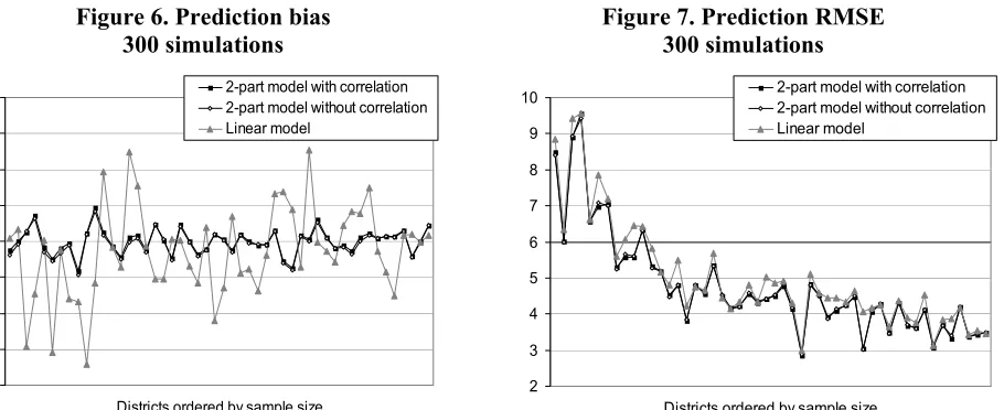
Figures 6 and 7 show the bias and root mean square error (RMSE) when predicting the true district means under the three models. Let ˆr

d

Y represent any of the three predictors for a given district d as obtained in simulation r, and denote by r

d

Y the corresponding true district mean. The bias and RMSE are defined as,

300 300 _{2 1/ 2}

1 1

ˆ ˆ

( r r) / 300 ; [ ( r r) / 300]

d r d d d r d d

Bias =

∑

₌ Y −Y RMSE =

∑

₌ Y −Y (11)

[image:13.595.69.524.70.256.2]

Figure 6. Prediction bias 300 simulations

-4 -3 -2 -1 0 1 2 3 4

Districts ordered by sample size

2-part model with correlation 2-part model without correlation Linear model

Figure 7. Prediction RMSE 300 simulations

2 3 4 5 6 7 8 9 10

Districts ordered by sample size

2-part model with correlation 2-part model without correlation Linear model

Evidently, fitting the linear mixed model without accounting for the accumulation of zero scores (Model C) yields appreciable biases, irrespective of the sample size. In some districts the absolute biases translate into relative biases of up to 15%. On the other hand, fitting the two-part model A or B, yields basically unbiased predictors. Fitting the linear mixed model yields also larger RMSEs, particularly for districts with small sample sizes, but the increase in RMSE compared to the other two models is not as big as in the case of the bias. This outcome is easily explained by the fact that the variances of the prediction errors are much smaller in the case of the linear mixed model, which is a much simpler model with fewer estimated parameters.

[image:14.595.164.460.100.261.2]

Figure 8. Percentage of confidence intervals covering the true mean

75 80 85 90 95 100

Districts ordered by sample size

2-part model with correlation 2-part model without correlation Linear model

6 Summary

The most important message emerging from this paper is that ignoring the accumulation of zeroes and fitting a linear mixed model can result in biased predictors and undercoverage of confidence intervals. Clearly, the magnitude of the bias and the undercoverage depends on the percentage of zero scores. Fitting a two-part model to such data yields unbiased predictors and confidence intervals with acceptable coverage rates. Fitting the full two-part model, accounting for the correlations between the random effects of the two parts is, in principle, the best choice, but it improved the predictions in our simulation study very marginally, which is probably explained by the low correlation of

ρ

_{u u, *}

=

0.26

used for generating the population data.

In this study we used MCMC simulations for fitting the models and computing the small area predictors and their variances, but as mentioned in Section 3, the use of this approach requires specifying prior distributions, which could affect the inference particularly with a small number of sampled areas. The other problem with the use of MCMC simulations is that it is extremely computing intensive. As mentioned earlier, we are presently investigating ways of overcoming the computation problems that we encountered with the use of the WinBUGS program. Another extension of the present study is to fit the full two part model following the frequency approach, using either MLwiN (Goldstein, 2003) or the aML software (Lillard and Panis, 2003).

References

Gelfand, A.E., and Smith, A.F.M (1990)

Sample-based approaches to calculating marginal densities. Journal of the American Statistical Association, 85, 072-985.

Goldstein, H. (2003)

Multilevel Statistical Models. Third edition. London, Edward Arnold:

Lillard, L.A., and Panis, C.W.A. (2003)

aML Multilevel Multiprocess Statistical Software, Version 2.0. EconWare, Los Angeles,

Olsen, M.K., and Schafer, J.L. (2001)

A two-part random effects model for semi-continuous longitudinal data. Journal of the

American Statistical Association, 96, 730-745.

Rao, J.N.K. (2003)

Small Area Estimation. New York: Wiley.

Raudenbush, S.W., Yang, M., and Yosef, M. (2000)

Maximum likelihood for generalized linear models with nested random effects via high-order, multivariate Laplace approximation. Journal of Computational and Graphical Statistics, 9, 141-157.

Spiegelhalter, D., Thomas, A., and Best, N.G. (2003)

Bayesian Inference using Gibbs Sampling. WinBUGS version 1.4, User manual. MRC

Biostatistics Unit, Institute of Public Health, Robinson Way, Cambridge, U.K.

Tanner, M. A. (1996)

Tools for Statistical Inference, 3rd edition. New York: Springer - Verlag

About the Authors

Danny Pfeffermann, Hebrew University, Israel, and University of Southampton, U.K.

Bénédicte Terryn, UNESCO Institute for Statistics, Montreal, Canada