Design effects in the analysis of longitudinal survey data

DESIGN EFFECTS IN THE ANALYSIS OF LONGITUDINAL SURVEY DATA

CHRIS SKINNER, MARCEL DE TOLEDO VIEIRA

ABSTRACT

The design effect measures the inflation of the sampling variance of an estimator as a result of the use of a complex sampling scheme. It is usually measured relative to the variance of the estimator under simple random sampling. Many social survey designs employ multi-stage sampling, leading to some clustering of the sample and this tends to lead to design effects greater than unity. There is some empirical evidence that design effects from clustering tend to decrease the more complex the analysis. For example, design effects for regression coefficients are often found to be less than design effects for the mean of the dependent variable in the regression. Evidence of design effects close to unity for such analyses may be used by some analysts of survey data to justify ignoring the sampling design in complex analyses. In this paper we present some evidence of an opposite tendency, for design effects to be higher for complex longitudinal analyses than for corresponding cross-sectional analyses. Our empirical evidence is based upon data from the British Household Panel Study. This survey follows longitudinally a sample of individuals selected in 1991 by two-stage sampling, with clustering by area. Data are collected in annual waves. Our analyses are based upon a subsample of women aged 16-39. The dependent variable is a gender role attitude score, derived from responses to six five-point questions, and treated as a continuous variable. Covariates include age group, economic activity and educational qualifications. Longitudinal regression models include random effects for women. Data are analysed for five waves of the survey when the gender role attitude questions were asked. The design effects for the regression coefficients are found to increase the more waves are included in the analysis. A similar tendency is observed for estimates of the time-averaged mean of the dependent variable. A possible theoretical explanation is provided. The implication of these findings is that standard errors in analyses of longitudinal survey data may be very misleading if the initial sample was clustered and if this clustering is ignored in the analysis.

Variance Estimation in the Analysis of Clustered Longitudinal

Survey Data

C. J. Skinner and M.D.T. Vieira

University of Southampton, United Kingdom

Summary. There is some empirical evidence that the variance-inflating impacts of

complex sampling schemes decline the more complex the analysis. In this paper we

present some evidence of an opposite tendency, for the impact to be higher for

longitudinal analyses than for corresponding cross-sectional analyses. Our

empirical evidence is based upon a regression analysis of longitudinal data on

gender role attitudes from the British Household Panel Survey. We investigate

reasons for this finding and suggest that it arises from a specific longitudinal feature

of the analysis. We contrast two approaches to allowing for the effect of clustering

in longitudinal analyses: a survey sampling approach and a multilevel modelling

approach. We suggest that the impact of clustering can be seriously

underestimated if it is simply handled by including an additive random effect to

represent the clustering in a multilevel model.

1. Introduction

This paper develops methodology for the analysis of complex survey data (Skinner et al.,

1989) to address longitudinal aspects of regression analyses of British Household Panel

Survey (BHPS) data on attitudes to gender roles and their relation to demographic and

economic variables. We consider two broad questions. First, is the impact of the complex

sampling design on variance estimation for analyses of these longitudinal data greater or

less than for corresponding cross-sectional analyses? Kish and Frankel (1974) presented

empirical work which suggested that the impacts of complex designs on variances are

reduced for more complex analytical statistics and so one might conjecture that the impact

on longitudinal analyses might also be reduced. We shall provide evidence in the opposite

direction that, at least for the specific analyses considered, the impact on longitudinal

analyses tends to be greater. Given that an impact does exist, the second question

addressed is how to undertake variance estimation. We shall focus in the paper on the

clustering impact of the sampling design. It is natural to represent such clustering via

multilevel models and we shall consider specifically how variance estimation methods

based upon multilevel models compare with survey sampling variance estimation

procedures.

When asking how an analysis should take account of complex sampling, it is natural

first to ask whether the parameters of interest should depend on the design, via the

population structure underlying the sampling (Skinner et al., 1989). In this paper we shall

assume this is not the case, since the primary sampling units in the BHPS are postcode

sectors, determined by the needs of the British postal system and assumed here not to be

relevant to the definition of parameters of scientific interest. A second question which

might be asked is how the sampling impacts on point estimation, e.g. via the use of

point estimation is unaffected by the design. Our main focus will be on the impact of the

design on variance estimation.

The impact on variance estimation will be measured here by the ‘misspecification

effect’, denoted meff (Skinner, 1989a), which is the variance of a point estimator divided by

the expectation of the variance estimator, a measure of relative bias of the variance

estimator. This concept is closely related to that of the ‘design effect’ or deff of Kish (1965),

defined as the variance of the point estimator under the given design divided by its

variance under simple random sampling with the same sample size, a concept more

relevant to the choice of design than to the choice of standard error estimator. In the

application in this paper, estimated meffs may be treated as equivalent to estimated deffs

when the variance estimator ignores the complex design.

One reason for studying meffs for variance estimators which ignore the design is

that analysts of longitudinal survey data face many difficult methodological challenges and

they may be tempted to view the impact of complex sampling on standard errors as a

relatively minor issue which, if ignored, is unlikely to lead to misleading inferences. Indeed,

in cases where the survey documentation indicates that the design effect of the mean of

the analyst’s outcome variable of interest is not much larger than one, the analyst might

justify ignoring the design when estimating standard errors by appealing to the observation

of Kish and Frankel (1974, p.13) that “design effects for complex statistics tend to be less

than those for means of the same variables”.

The paper is motivated by a regression analysis of five waves of BHPS data, based

upon work of Berrington (2002) and described in Section 2. After a description of models

and estimation methods in Section 3, the paper proceeds in Section 4 to provide evidence

that meffs for longitudinal analyses can be greater than for corresponding cross-sectional

analyses, implying that more caution is required before ignoring the complex design in

Section 5, with the focus being on the treatment of clustering and on a comparison

between a multilevel modelling approach (Goldstein, 2003, Ch.9; Renard and

Molenberghs, 2002) and a survey sampling approach (Skinner et al, 1989).

We ignore the effects of stratification and weighting in the empirical work in sections

4 and 5 in order to isolate the source of potential misspecification effects and to avoid

introducing the more complex weighting issues arising with multilevel models (Pfeffermann

et al., 1998). We make brief remarks on these effects in the concluding discussion in

Section 6.

2. The motivating application to BHPS data

Recent decades have witnessed major changes in the roles of men and women in the

family in many countries. Social scientists are interested in the relation between changing

attitudes to gender roles and changes in behaviour, such as parenthood and labour force

participation (e.g. Morgan and Waite, 1987; Fan and Marini, 2000). A variety of forms of

statistical analysis are used to provide evidence about these relationships. In this paper we

consider a longitudinal regression analysis, based upon a model considered by Berrington

(2002), with a measure of attitude to gender roles as the dependent variable. We also

consider some simpler versions of this analysis to facilitate understanding of the

methodological issues outlined in Section 1. The models will be set out formally in Section

3.

The data come from waves 1, 3, 5, 7 and 9 (collected in 1991, 1993, 1995, 1997,

and 1999 respectively) of the BHPS, when respondents were asked whether they ‘strongly

agreed’, ‘agreed’, ‘neither agreed nor disagreed’, ‘disagreed’ or ‘strongly disagreed’ with a

series of statements concerning the family, women’s roles, and work out of the household.

Responses were scored from 1 to 5. Factor analysis was used to assess which

considered here is the total score for six selected statements. Higher scores signify more

egalitarian gender role attitudes. Berrington (2002) provides further discussion of this

variable.

Covariates for the regression analysis were selected on the basis of discussion in

Berrington (2002) but reduced in number to facilitate a focus on the methodological issues

of interest. The covariate of primary scientific interest is economic activity, which

distinguishes in particular between women who are at home looking after children

(denoted ‘family care’) and women following other forms of activity in relation to the labour

market. Variables reflecting age and education are also included since these have often

been found to be strongly related to gender role attitudes (e.g. Fan and Marini, 2000). All

these covariates may change values between waves. A year variable (scored 1, 3,…, 9) is

also included. This may reflect both historical change and the general ageing of the

women in the sample.

The BHPS is a household panel survey of individuals in private domiciles in Great

Britain (Taylor et al., 2001). Given the interest in whether women’s primary labour market

activity is ‘caring for a family’, we define our study population as women aged 16-39 in

1991. This results in a subset of data on n = 1340 women. This subset consists of those

women in the eligible age range for whom full interview outcomes (complete records) were

obtained in all the five waves. We comment further on the treatment of nonresponse in

section 3.

The initial (wave one) sample of the BHPS in 1991 was selected by a stratified

multistage design in which households had approximately equal probabilities of inclusion.

As primary sampling units (PSUs), 250 postcode sectors were selected, with replacement

and with probability of selection proportional to size using a systematic procedure.

Addresses were selected as secondary sampling units, with the adoption of an analogous

included, and in those with more than 3 households, a random selection procedure, using

a Kish grid, was used for the selection of 3 households. Then, all resident household

members aged 16 or over were selected. All adults selected at wave one, were followed

from wave two and beyond. A consequence of this design is that inclusion probabilities of

adults vary little. The impact of weighting is considered briefly in section 6. The 1340

women represented in the data are spread fairly evenly across 248 postcode sectors. The

small average sample size of around five per postcode sector combined with the relatively

low intra-postcode sector correlation for the attitude variable of interest leads to relatively

small impacts of the design, as measured by meffs. Since our aims are methodological

ones, to compare meffs for different analyses, we have chosen to group the postcode

sectors into 47 geographically contiguous clusters, to create sharper comparisons, less

blurred by sampling errors which can be appreciable in variance estimation. The meffs in

the tables we present therefore tend to be greater than they are for the actual design. The

latter results tend to follow similar patterns, although the patterns are less clear-cut as a

result of sampling error.

3. Regression model and inference procedures

Let y_itdenote the value of the attitude score for woman

i

at wave

t

(coded

t

=

1,...,

T

=

5

to correspond to 1991, 1993, …,1999) and let

y

i

=

( ,...,

y

i₁

y

iT

)’

be the vector of repeated measures. We consider linear models of the following form to represent the expectation of

i

y

given the values of covariates:

( )

i i

E y

=

x

β

, (1)

where

x

i

=

( ’,...,

x

i₁

x

iT

’)’

,

x

itis a 1×q vector of specified values of covariates for woman i

at wave t ,

β

is the q×1 vector of regression coefficients and the expectation is with

analysis might include a measurement error model for attitudes (e.g. Fan and Marini,

2000), with each of the five-point responses to the six statements treated as ordinal

variables. Here, we adopt a simpler approach, treating the aggregate score

y

_it and the associated coefficient vector

β

as scientifically interesting, with the measurement error

included in the error term of the model.

We consider estimation of

β

based on data from the ‘longitudinal sample’,

s

_T, i.e. the sample for which observations are available for each of

t

=

1,...,

T

. We did not attempt to use data observed only at a subset of the five waves, partly for simplicity but also

because our primary interest is clustering and we did not wish differences in clustering

effects over time to be confounded with differences in incomplete data effects. A concern

with the use of the longitudinal sample

s

_T is that the underlying attrition process may lead to biased estimation of

β

. One possible way of attempting to correct for this potential

biasing effect is via the use of longitudinal survey weights,

w i s

iT

,

∈

(Lepkowski, 1986). The most general estimator of

β

we consider is

(

)

1

1 1

ˆ

_'

_'

T T

iT i i iT i i

i s

w x V x

i s

w x V y

β

− − −

∈∑ ∈∑

=

, (2)

where

V

is a ‘working’ variance matrix of

y

_i (Diggle et al. 2002, p.70), taken as the

exchangeable variance matrix with diagonal elements

σ

2 _{and off-diagonal elements}

ρσ

_ˆ

2_,

and

ρ

ˆ

is an estimator of the intra-individual correlation, obtained by iterating between

generalised least squares estimation of

β

and survey-weighted moment-based estimation

of the intra-individual correlation (Liang and Zeger, 1986; Shah et al., 1997). Note that

σ

2

cancels out in (2) and hence does not need to be estimated for

β

ˆ

.

it it i it

y

=

x

β

+ +

u v

, (3)

with independent random effects

u

_i and

v

_it with variances

σ

_u2

=

ρσ

2 and

2

₍₁

₎

2

v

σ

= −

ρ σ

respectively. We find that this model provides a first approximation to the

variance structure for the regression models fitted in section 4. For illustration, we find

ˆ 0.59

ρ

=

in the most elaborate regression model implying a fairly substantial

between-woman component in the attitude scores unexplained by the chosen covariates. It is not

necessary, however, for the error structure to follow the specific model in (3) exactly for

β

ˆ

to be consistent.

To estimate the covariance matrix of

β

ˆ

allowing for the complex sampling design,

we may use the linearization estimator (Skinner, 1989b, p.78):

1 1

-1 2 -1

ˆ

( )

'

V

/(

1) (

)

'

V

T T

iT i i h h ha h iT i i

i s h a i s

v

β

w x

x

n n

z

z

w x

x

− −

∈ ∈





_

_





=

_

_

_

−

−

_

_

_







∑



∑

∑



∑



, (4)

where

h

denotes stratum,

a

denotes area (primary sampling unit, PSU),

n

_h is the

number of PSUs in stratum

h

,

_’

1

i

ha iT i i

z

_{= ∑}

w x V e

− _,

_/

a

h ha a

z

_{= ∑}

z n

and

e

_i

= −

y

_i

x

_i

β

ˆ

. Note

that this variance estimator requires use of the stratum and primary sampling unit

identifiers. See Lavange et al. (1996) and Lavange et al. (2001) for applications of a similar

approach to allowing for complex sampling designs in regression analyses of repeated

measures data from different longitudinal studies.

In order to assess the impact of the complex design on variance estimation, we also

consider a linearization variance estimator which ignores the complex design, denoted

0

( )

ˆ

v

β

, given by expression (4) where the PSUs become the same as women so that

z

_hais

replaced by 1

’

iT i i

w x V e

− _{and there is only a single stratum so that}

h

n

=

n

is the overall

is the ‘robust’ variance estimator presented by Liang and Zeger (1986) as consistent

when (1) holds, but where the working variance matrix,

V

, may not reflect the true variance structure. See also Diggle et al. (2002, section 4.6).

Following Skinner (1989a, p.24), we refer to

v

( ) / ( )

β

ˆ

_k

v

₀

β

ˆ

_k , the ratio of these two

variance estimators for the _kth _{element of}

β

ˆ

_{, as an estimated misspecification effect and}

denote it meff. This ratio may be viewed as an estimator of the misspecification effect,

defined as

var( ) / [ ( ]

β

ˆ

k

E v

₀

β

ˆ

k , on the assumption that

v

( )

β

ˆ

is a consistent estimator of

ˆ

var( )

β

. This quantity is a measure of the relative bias of the ‘incorrectly specified’

variance estimator

v

₀

( )

β

ˆ

k as an estimator of

var( )

β

ˆ

k .

In general, meffs will reflect the impact of weighting, clustering and stratification. For

simplicity of interpretation, we shall in this paper only present values of meffs capturing the

effect of clustering, treating the weights as constant and ignoring stratification.

4. Misspecification effects: the impact of ignoring clustering in longitudinal

analyses

In this section we explore the impact of ignoring clustering in standard error estimation for

various longitudinal analyses. To provide theoretical motivation for the kind of impact we

may expect, consider converting the two-level model in (3) into a simple three-level model

(Goldstein, 2003) as:

ait ait a ai ait

y

=

x

β η

+ +

u

+

v

, (5)

where an additional subscript

a

has been added to denote area (cluster) and an additional random term

η

_a with variance 2

η

σ

represents the area effect (assumed independent of

u

_ai

of cross-sectional analyses, where

t

is kept fixed as

t

=

1

. In this case, if we suppose for simplicity that

x

ait

≡

1

and

β

is the mean of

y

ait in (5) and that there is a common sample

size

m

per cluster, the misspecification effect is approximately equal to

1 (

+

m

−

1)

τ

1,

where

τ σ σ

₁

=

η2

/(

η2

+

σ

_u2

+

σ

_v2

)

is the intracluster correlation (Skinner, 1989b, p. 38). If the

sample sizes per cluster are unequal a common approximation is to replace

m

in this formula by

m

, the average sample size per cluster.

Turning to the longitudinal case, where again

x

ait

≡

1

and now

β

is a longitudinal

mean of

y

_ait for

t

=

1,...,

T

, the same theory for misspecification effects will apply, but

where

τ

₁ is replaced by

τ

, the intracluster correlation for

η

_a and

u

_ai

+

v

_ait averaged over

the waves., i.e.

τ σ σ

=

η2

/(

η2

+

σ

u2

+

σ

v2

/ )

T

. Hence, under this model, the misspecification

effect increases as

T

increases, if

σ

v2

>

0

.

Let us now compare this expected theoretical pattern with the empirical findings.

Using data from just the first wave and setting

x

ait

≡

1

, the meff for this cross-sectional mean is given in Table 1 as about 1.5. This value is plausible since the average sample

size per cluster is

m

=

1340/ 47 29

≈

and using the

1 (

+

m

−

1)

τ

1 formula, the implied

value of

τ

₁ is about 0.02 and such a small value is in line with other estimated values of

τ

₁

found for attitudinal variables in British surveys (Lynn and Lievesley, 1991, App. D).

To assess the impact of the longitudinal aspect of the data, we re-estimate the meff

using data for waves 1,…,t for t=2, 3, … 5. Table 1 suggests a tendency for the meff to

increase with the number of waves, as anticipated from the theoretical reasoning. These

meffs are certainly subject to sampling error and there appears to be some genuine

variation in misspecification effects for cross-sectional estimates at different waves but this

To pursue the theoretical rationale for this finding further, note that model (5) is

likely to be an oversimplification because the area effects are likely to display some

variation over time, suggesting that we write

η

_at rather than

η

_a. In this case,

τ

becomes

var( ) /[var( ) var(

a a

u

a

v

a

)]

τ

=

η

η

+

+

, where

η

a

= ∑

t

η

at

/

T

and

u

a

+ =

v

a

(

) /

t

u

ai

+

v

ait

T

∑

. Now, it seems plausible that the average level of egalitarian attitudes in

an area will vary less from year to year than the attitude scores of individual women, since

the latter will be affected both by measurement error and genuine changes in attitudes, so

that

var( )

η

a may be expected to decline more slowly with

T

than

var(

u

a

+

v

a

)

. We may

therefore expect

τ

, and consequently the meff, to increase as

T

increases, as we observe in Table 1.

We next elaborate the analysis by including indicator variables for economic activity

as covariates. The resulting regression model has an intercept term and four covariates

representing contrasts between women who are employed full-time and women in other

categories of economic activity. The meffs are presented in Table 2. The intercept term is

a domain mean and standard theory for a meff of a mean in a domain cutting across

clusters (Skinner, 1989b, p.60) suggests that it will be somewhat less than the meff for the

mean in the whole sample, as indeed is observed with the meff for the cross-section

domain mean of 1.13 in Table 2 being less than the value 1.51 in Table 1. As before, there

is some evidence in Table 2 of tendency for the meff to increase, from 1.13 with one wave

to 1.50 with five waves, albeit with lower values of the meffs than in Table 1. The meffs for

the contrasts in Table 2 vary in size, some greater than and some less than one. These

meffs may be viewed as a combination of the traditional variance inflating effect of

clustering in surveys together with the familiar variance reducing effect of blocking in an

experiment. The main feature of these results of interest here is that there is again no

tendency for the meffs to converge to one as the number of waves increases. If there is a

between women who are full-time employed and those who are ‘at home caring for a

family’, the meff is consistently well below one.

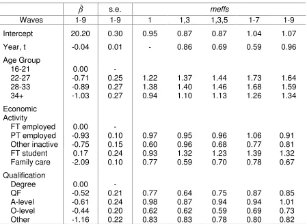
We next refine the model further by including, as additional covariates, age group,

year and qualifications. The results for meffs are given in Table 3. The meffs for the

economic activity covariates again vary, some being above one and some below one.

There is again some evidence of a tendency for these meffs to diverge away from one as

the number of waves increases. A comparison of Tables 1 and 3 confirms the observation

of Kish and Frankel (1974) that meffs for regression coefficients tend not to be greater

than meffs for the means of the dependent variable.

5. Alternative approaches to variance estimation

It follows from the previous section that it is, in general, important to allow for clustering in

variance estimation with longitudinal survey data. Evidence was presented that the effect

of ignoring clustering was at least as great for certain longitudinal analyses as

cross-sectional analyses. The linearization estimator in (4) provides one approach to variance

estimation. In this section we compare this estimator with a model-based approach.

In a model-based approach, we may aim to capture the effect of clustering on

variances by the inclusion of the random area effects,

η

_a, in the three-level model in (5)

and by the use of an estimation approach which encompasses both point and interval

estimation. We consider here the use of iterative generalized least squares (IGLS),

following Goldstein (1986). This leads to a slightly different point estimator of

β

to the

estimator in (2) but we found almost identical values of these two estimators in our

application.

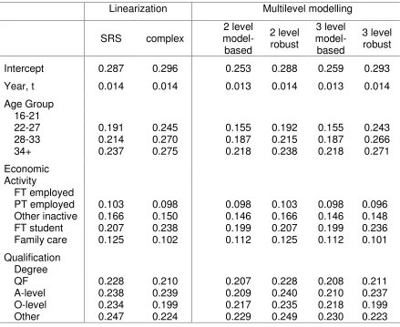
We next estimated the standard errors for the

β

estimates, using the IGLS

procedure (Goldstein, 1986), under the assumption that model (5) holds with each of the

are given in Table 4 in the column headed ‘3 level model-based’. For comparison, we also

estimate the standard errors under the two level model in (3) – the results are in the

column headed ‘2 level model-based’. The estimates in the two columns are virtually

identical. There is a single digit difference in the third decimal place for some coefficients

and slightly greater difference for the intercept term. We suggest that this is evidence that

simply adding in a random area effect term can seriously understate the impact of

clustering on the standard errors of the estimated regression coefficients. To provide

theoretical support for this claim, consider first the cross-sectional case (

T

=

1

) where

x

is scalar. Then, if the three-level model (5) holds, an approximate expression for the meff of

the variance estimator of

β

ˆ

based upon the two-level model (3) is:

1

1 (

1)

_x

meff

= +

m

−

τ τ

, (6)

where

τ

₁ is as above and

τ

_xis the intracluster correlations for

x

(Scott and Holt, 1982; Skinner, 1989b, p.68). This result extends in the longitudinal case, to:

1

≤

meff

≤ +

1 (

m

−

1)

ττ

_z, (7)

where

τ

is the long-run (

T

= ∞

) version of

τ

(see Appendix) and

τ

z is an intracluster

correlation coefficient for

z

_ai

=

∑

_t

x

_ait

/

T

. The proof of this result and the simplifying

assumptions required are sketched in the Appendix. The main point is that both

τ

and

τ

z

are small in our application and hence

ττ

_zwill be very small and thus the meff will be close

to one. In our application, the estimated value of

τ

is 0.019 and none of the covariates

may be expected to display important intra-area correlation. This theoretical result

provides one possible explanation for the negligible size of the differences in standard

errors observed in Table 3 between the two-level and three-level models.

As discussed in Skinner (1989b, p.68) and supported by theory in Skinner (1986),

the main feature of clustering likely to impact on the standard errors of estimated

not allowed for in model (5). We have explored this idea by introducing random coefficients

in the model. Treating the elements of

β

now as the expected values of the random

coefficients, we found that the estimates of

β

were hardly changed. We found that the

estimated standard errors of these estimates were indeed inflated, much more so than

from the introduction of the single term

η

_a, and that the inflation was of an order similar to

those of the meffs in Tables 2 and 3. Nevertheless, the IGLS method did lead to several

negative estimates of the variances of the random coefficients, raising issues of which

coefficients to allow to vary or more generally the issue of model specification. This

problem is accentuated with increasing numbers of covariates, as the number of

parameters in the covariance matrix of the coefficient vector increases with the square of

the number of covariates. Overall, the inclusion of random coefficients seems to raise at

least as many problems as it solves, if the clustering is not of intrinsic scientific interest,

and thus does not seem a very satisfactory way to allow for clustering in variance

estimation. It is simpler to change the method of variance estimation.

One approach is to use a variance estimator which allows for the kind of

heteroskedasticity which random coefficients would generate, treating differences between

random coefficients and their expectation

β

as contributing to the error component of the

model. This is achieved for IGLS or other likelihood-based point estimation methods for

the multilevel model in (5) by the use of a ‘robust’ variance estimation method (Goldstein,

2003, p. 80). These robust variance estimation methods turn out to be almost the same as

the linearization method of section 3. Values of these robust standard error estimates are

also included in Table 4. The robust standard error estimator for the two level model

performs very similarly to the linearization estimator which ignores clustering. The robust

standard error estimator for the three level model performs very similarly to the

the differences between the estimation method for

V

in (2) and (4) and the IGLS estimation method.

The linearization method in the presence of two-stage sampling is thus very close to

robust variance estimation methods used in the literature on multilevel modeling. The

distinction between the methods becomes stronger if we allow also for stratification and

weighting. Another distinction is that in the multilevel modeling approach, differences

between model-based and the robust standard errors might be used as a diagnostic tool to

detect departures from the model (Maas and Hox, 2004). For example, the large

differences in the three-level standard errors for the coefficients of age group in Table 4

might lead to consideration of the inclusion of random coefficients for age group. This

contrasts with the survey sampling approach where the error structure in model (5) is only

treated as a working model and it is not necessarily expected that standard errors based

upon this model will be approximately valid.

In this paper we have implicitly treated the linearization method as a ‘gold standard’

for variance estimation because of its consistency. Nevertheless, this method may be

expected to be less efficient than model-based variance estimation if the model is correct

and the variance of the variance estimator should not be ignored, especially when the

number of clusters is not large. Wolter (1985, Ch. 8) summarises a number of simulation

studies investigating both the bias and variance of the linearization variance estimator and

these studies suggest that the linearization method performs well even with few clusters.

Possible degrees of freedom corrections to confidence intervals for regression coefficients

based upon the linearization method with small numbers of clusters are discussed by

Fuller (1984). A simulation study of estimators for multilevel models in Maas and Hox

(2004) does not suggest that the linearization method performs noticeably worse than the

model-based approach, in terms of the coverage of confidence intervals for coefficients in

6. Discussion

We have presented some theoretical arguments and empirical evidence that the impact of

ignoring clustering in standard error estimation for certain longitudinal analyses can tend to

be larger than for corresponding cross-sectional analyses. The implication is that it is, in

general, at least as important to allow for clustering in standard error estimation for

longitudinal analyses as for cross-sectional analyses. Thus, the expectation from the

finding of Kish and Frankel (1974) that complex sampling has less of an impact on

variances for more complex analytical statistics was not borne out in this case.

The longitudinal analyses considered in this paper are of a certain kind and we

should emphasise that the patterns observed for meffs in these kinds of analyses may well

not extend to other kinds of longitudinal analyses. To speculate about the class of models

and estimators for which the patterns observed in this paper might apply, we conjecture

that increased meffs for longitudinal analyses will arise when the longitudinal design

enables temporal ‘random’ variation in individual responses to be extracted from

between-person differences and hence to reduce the component of standard errors due to these

differences, but provides less ‘explanation’ of between cluster differences, so that the

relative importance of this component of standard errors becomes greater.

The empirical work presented in this paper has also been restricted to the impact of

clustering. We have undertaken corresponding work allowing for weighting and

stratification and found broadly similar findings. Stratification tends to have a smaller effect

than clustering. The sample selection probabilities in the BHPS do not vary greatly and the

impact of weighting by the reciprocals of these probabilities on both point and variance

estimates tends not to be large. There is rather greater variation among the longitudinal

attrition occurs, the weights,

w

_iT, tend to become more variable and lead to greater inflation of variances. This tends to compound the effect we have described of meffs

increasing with

T

.

Leaving aside consideration of stratification and weighting, we have compared two

approaches to allowing for cluster sampling. We have treated the survey sampling

approach as a benchmark. We have also considered a multilevel modelling approach to

allow for clustering. We have suggested that the use of a simple additive random effect to

represent clustering can seriously understate the impact of clustering and may lead to

underestimation of standard errors. If the clustering is of scientific interest, the solution is

to consider the specification of the model, including for example the use of random

coefficients. If the clustering is treated as a nuisance, simply reflecting administrative

convenience in data collection, we suggest the survey sampling approach has a number of

practical advantages. This is discussed further by Lavange et al. (1996, 2001) in relation to

other applications to repeated measures data

Appendix. Justification for (7)

For simplicity,

x

and

β

are taken to be scalar,

β

ˆ

is taken to be the ordinary least squares estimator and it is assumed that the sample sizes within clusters are all equal to

m

. The

meff in (7) is defined as

var ( ) / [ ( )]

₃

β

ˆ

E v

_{3 2}

β

ˆ

, where

E

₃ and

var

₃ are moments with

respect to the three-level model in (5) and

v

₂

( )

β

ˆ

is a variance estimator based upon the two-level model in (3). Under (5) we obtain

2 2 2 2 2 2 2 2

3

ˆ

var ( ) (

_cit

) (

_{c u ci v cit}

)

cit c ci cit

x

_η

x

x

x

β

−

σ

σ

σ

++ +

where + denotes summation across a suffix,

σ σ

_η2

,

_u2and

σ

_v2 are the respective variances

of

η

_a

,

u

_ai and

v

_aitand

x

_citis centred at 0. We further suppose that

v

₂

( )

β

ˆ

is defined so that

2 2 2 2 2 2 2

2

ˆ

[ ( )] (

cit

) [(

u

)

ci v cit

]

cit ci cit

E v

β

x

−

σ

_η

σ

x

σ

x

+

≈

∑

+

∑

+

∑

.

After some algebra we may show that

1 (

1)

_z

[1 (

1) ]/[1 (

_x

1)

_x

]

meff

= +

m

−

ττ ρ

+

T

−

τ

+

T

−

ρτ

, (8)

where

τ σ σ

=

_η2

/(

_η2

+

σ

_u2

)

,

ρ σ

=

(

_η2

+

σ

_u2

) /(

σ

_η2

+

σ

_u2

+

σ

_v2

)

,

τ

_x

=

σ σ

_xB2

/

_x2,

2 2

_/(

₎

x _cit

x

cit

nT

σ

=

∑

,

σ

_xB2

=

[

∑

_ci

(

x

_ci+

/ ) /

T

2

n

−

σ

_x2

/ ]/[1 1/ ]

T

−

T

,

τ

_z

=

σ σ

_zB2

/

_z2,

2 2

_/

z _ci

z n

ci

σ

=

∑

,

σ

_zB2

=

[

∑

_c

(

z

_c+

/ ) /

m

2

C

−

σ

_z2

/ ]/[1 1/ ]

m

−

m

and

n Cm

=

is the sample

size. Note that when

T

=

1

, we have

ρ

=

1

and (8) reduces to (6). In general

ρ

≤

1

and (7) follows from (8). In fact, we estimate

ρ

as 0.59 in our application so the bound in (7) is

not expected to be very tight.

References

Berrington, A. (2002) Exploring relationships between entry Into parenthood and gender role attitudes: evidence from the British Household Panel Study. In Lesthaeghe, R. ed.

Meaning and Choice: Value Orientations and Life Course Decisions. Brussels: NIDI. Diggle, P. J., Heagerty, P., Liang, K. & Zeger, S. L. (2002) Analysis of Longitudinal Data.

2nd _{ed. Oxford: Oxford University Press.}

Fan, P.-L. and Marini, M.M. (2000) Influences on gender-role attitudes during the transition to adulthood. Social Science Research, 29, 258-283.

Fuller, W.A. (1984) Least squares and related analyses for complex survey designs.

Survey Methodology, 10, 97-118.

Goldstein, H. (1986) Multilevel mixed linear model analysis using iterative generalised least squares. Biometrika, 74, 430-431.

Kish, L. and Frankel, M. R. (1974) Inference from complex samples. J. R. Statist. Soc. B,

36, 1-37.

Lavange, L.M., Koch, G.G. and Schwartz, T.A. (2001) Applying sample survey methods to clinical trials data. Statistics in Medicine, 20, 2609-23.

Lavange, L.M., Stearns, S.C., Lafata, J.E., Koch, G.G. and Shah, B.V. (1996) Innovative strategies using SUDAAN for analysis of health surveys with complex samples.

Statistical Methods in Medical Research, 5, 311-329.

Lepkowski, J.M. (1986) Treatment of wave nonresponse in panel surveys. In Kasprzyk, D., Duncan, G., Kalton, G. and Singh, M.P. eds. Panel Surveys. New York: Wiley.

Liang, K.Y. and Zeger, S.L. (1986) Longitudinal data analysis using generalized linear models. Biometrika, 73, 13-22.

Lynn, P. and Lievesley, D. (1991) Drawing General Population Samples in Great Britain. London: Social and Community Planning Research.

Maas, C.J.M and Hox, J.J. (2004) The influence of violations of assumptions on multilevel parameter estimates and their standard errors. Comp. Statist. Data Analysis, 46, 427-440.

Morgan, S.P. and Waite, L.J. (1987) Parenthood and the attitudes of young adults. Am. Sociological Review, 52, 541-547.

Pfeffermann, D., Skinner, C., Holmes, D., Goldstein, H. and Rasbash, J. (1998) Weighting for unequal selection probabilities in multilevel models. J. R. Statist. Soc. B, 60, 23-56. Renard, D. and Molenberghs, G. (2002) Multilevel modelling of complex survey data. In

Topics in Modelling Clustered Data ( eds. Aerts, M., Geys, H., Molenberghs, G. and Ryan, L.M.), pp. 263-272. Boca Raton: Chapman and Hall/CRC.

Scott, A.J. and Holt, D. (1982) The effect of two stage sampling on ordinary least squares methods. J.Amer. Statist. Ass.,77, 848-854.

Shah, B. V., Barnwell, B.G. and Bieler, G.S. (1997) SUDAAN User’s Manual, Release 7.5. Research Triangle Park, NC: Research Triangle Institute.

Skinner, C.J. (1986) Design effects of two stage sampling. J.R. Statist. Soc. B, 48, 89-99. Skinner, C. J. (1989a) Introduction to Part A. In Skinner, C. J., Holt, D. and Smith, T. M. F.

eds. Analysis of Complex Surveys. Chichester: Wiley, pp.23-58.

Skinner, C. J. (1989b) Domain means, regression and multivariate analysis. In Skinner, C. J., Holt, D. and Smith, T. M. F. eds. Analysis of Complex Surveys. Chichester: Wiley, pp. 59-87.

Taylor, M. F. ed, with Brice J., Buck, N. and Prentice-Lane E. (2001) British Household Panel Survey - User Manual - Volume A: Introduction, Technical Report and Appendices. Colchester, University of Essex.

[image:22.612.79.514.70.120.2]

Table 1. Estimates for Longitudinal Means

βˆ s.e. meffs

Waves 1-9 1-9 1 1,3 1,3,5 1-7 1-9

[image:22.612.75.530.175.302.2]

19.83 0.12 1.51 1.50 1.68 1.81 1.84

Table 2. Estimates for Regression with Covariates defined by Economic Activity

βˆ s.e. meffs

Waves 1-9 1-9 1 1,3 1,3,5 1-7 1-9

Intercept 20.58 0.11 1.13 1.01 1.09 1.38 1.50

Contrasts for

PT employed -1.03 0.10 0.93 0.91 0.93 1.00 0.89

Other inactive -0.80 0.15 0.60 0.96 0.68 0.76 0.81

FT student 0.41 0.24 1.10 1.32 1.14 1.48 1.44

Family care -2.18 0.10 0.72 0.49 0.58 0.66 0.60

Note: intercept is mean for women full-time employed

contrasts are for other categories of economic activity relative to full-time employed

Table 3. Estimates for Regression Coefficients with Additional Covariates in Model

βˆ _{s.e. meffs}

Waves 1-9 1-9 1 1,3 1,3,5 1-7 1-9

Intercept 20.20 0.30 0.95 0.87 0.87 1.04 1.07

Year, t -0.04 0.01 - 0.86 0.69 0.59 0.96

Age Group

16-21 0.00 -

22-27 -0.71 0.25 1.22 1.37 1.44 1.73 1.64

28-33 -0.89 0.27 1.38 1.40 1.46 1.68 1.59

34+ -1.03 0.27 0.94 1.10 1.13 1.26 1.34

Economic Activity

FT employed 0.00 -

PT employed -0.93 0.10 0.97 0.95 0.96 1.06 0.91

Other inactive -0.75 0.15 0.60 0.96 0.68 0.77 0.81

FT student 0.17 0.24 0.93 1.32 1.23 1.39 1.32

Family care -2.09 0.10 0.77 0.59 0.70 0.78 0.67

Qualification

Degree 0.00 -

QF -0.52 0.21 0.77 0.64 0.75 0.87 0.85

A-level -0.61 0.24 0.98 0.87 0.94 0.94 1.01

O-level -0.44 0.20 0.62 0.62 0.59 0.69 0.73

Other -1.16 0.22 0.83 0.83 0.78 0.80 0.82

[image:22.612.80.529.370.698.2]

[image:23.612.80.519.90.449.2]

Table 4. Estimated Standard Errors of Regression Coefficients

Linearization Multilevel modelling

SRS complex model-2 level based

2 level robust

3 level model-based

3 level robust

Intercept 0.287 0.296 0.253 0.288 0.259 0.293

Year, t 0.014 0.014 0.013 0.014 0.013 0.014

Age Group 16-21

22-27 0.191 0.245 0.155 0.192 0.155 0.243

28-33 0.214 0.270 0.187 0.215 0.187 0.266

34+ 0.237 0.275 0.218 0.238 0.218 0.271

Economic Activity

FT employed

PT employed 0.103 0.098 0.098 0.103 0.098 0.096

Other inactive 0.166 0.150 0.146 0.166 0.146 0.148

FT student 0.207 0.238 0.199 0.207 0.199 0.236

Family care 0.125 0.102 0.112 0.125 0.112 0.101

Qualification Degree

QF 0.228 0.210 0.207 0.228 0.208 0.211

A-level 0.238 0.239 0.209 0.240 0.210 0.237

O-level 0.234 0.199 0.217 0.235 0.218 0.199