The causes of the red sequence, the blue cloud, the green valley, and the green mountain

MNRAS481,1183–1194 (2018) doi:10.1093/mnras/sty2220 Advance Access publication 2018 August 23

The causes of the red sequence, the blue cloud, the green valley,

and the green mountain

Stephen A. Eales,

Maarten Baes,

Nathan Bourne,

Malcolm Bremer,

Michael J. I. Brown,

Christopher Clark,

David Clements,

Pieter de Vis,

Simon Driver,

Loretta Dunne,

Simon Dye,

Cristina Furlanetto,

Benne Holwerda,

R. J. Ivison,

L. S. Kelvin,

Maritza Lara-Lopez,

Lerothodi Leeuw,

Jon Loveday,

Steve Maddox,

Michał J. Michałowski,

Steven Phillipps,

Aaron Robotham,

Dan Smith,

Matthew Smith,

Elisabetta Valiante,

Paul van der Werf

and Angus Wright

Affiliations are listed at the end of the paper

Accepted 2018 August 10. Received 2018 August 8; in original form 2018 March 28

A B S T R A C T

The galaxies found in optical surveys fall in two distinct regions of a diagram of optical colour versus absolute magnitude: the red sequence and the blue cloud, with the green valley in between. We show that the galaxies found in a submillimetre survey have almost the opposite distribution in this diagram, forming a ‘green mountain’. We show that these distinctive distributions follow naturally from a single, continuous, curved Galaxy Sequence in a diagram of specific star formation rate versus stellar mass, without there being the need for a separate star-forming galaxy main sequence and region of passive galaxies. The cause of the red sequence and the blue cloud is the geometric mapping between stellar mass/specific star formation rate and absolute magnitude/colour, which distorts a continuous Galaxy Sequence in the diagram of intrinsic properties into a bimodal distribution in the diagram of observed properties. The cause of the green mountain is Malmquist bias in the submillimetre waveband, with submillimetre surveys tending to select galaxies on the curve of the Galaxy Sequence, which have the highest ratios of submillimetre-to-optical luminosity. This effect, working in reverse, causes galaxies on the curve of the Galaxy Sequence to be underrepresented in optical samples, deepening the green valley. The green valley is therefore not evidence (1) for there being two distinct populations of galaxies, (2) for galaxies in this region evolving more quickly than galaxies in the blue cloud and the red sequence, and (3) for rapid-quenching processes in the galaxy population.

Key words: galaxies: evolution – galaxies: general.

1 I N T R O D U C T I O N

Galaxies discovered in optical surveys fall in two main areas of a diagram of optical colour versus absolute magnitude: a narrow band of galaxies with red colours, commonly called the ‘red sequence’, and a more diffuse ‘blue cloud’. In between these two regions there are still galaxies, but fewer, and this region is commonly called the ‘green valley’. The existence of the red sequence has been known for over 50 yr (Baum1959), and the form of the rest of the distribu-tion has gradually become clear over the intervening decades (e.g.

_{E-mail:sae@astro.cf.ac.uk}

Visvanathan1981), with a big increase in our knowledge coming with the release of the huge galaxy catalogues produced from the Sloan Digital Sky Survey (SDSS; Strateva et al.2001; Bell et al. 2003).

The obvious interpretation of this diagram (we will argue in this paper that it is not necessarily the correct one) is that there are two physically distinct classes of galaxy. Additional evidence in favour of this interpretation is that the morphologies of the galaxies in the two classes are also generally different, with the galaxies in the red sequence mostly being early-type galaxies (ETGs) and the blue-cloud galaxies generally being late-type galaxies (LTGs), although

2018 The Author(s)

the correspondence is not perfect and the exceptions have spawned an entire literature (Cortese2012,and references therein).

Once the form of this distribution had become clear, the natural next step was to go beyond plotting colour–magnitude diagrams and instead plot real physical properties of galaxies. Since blue colours indicate a galaxy with a high specific star formation rate (star forma-tion rate divided by stellar mass, SSFR), with red colours indicating the opposite, and absolute magnitude being approximately propor-tional to stellar mass, a natural diagram to plot was SSFR versus stellar mass. Most of the early papers concluded that galaxies fall in two distinct regions of this diagram. This time, because of the map-ping between colour and SSFR, the blue galaxies fell in a narrow band, which was given the name the ‘main sequence’ or the ‘star-forming main sequence’, while the red sequence became a region separated from and below the main sequence, with the galaxies in this region being either called ‘red and dead’, ‘quiescent’, or ‘quenched’ (Daddi et al.2007; Elbaz et al.2007; Noeske et al. 2007; Peng, Maiolino & Cochrane2010; Rodighiero et al.2011).

The consequence of there being two physically distinct classes of galaxy is profound. ‘Red and dead’ galaxies cannot always have been dead because they contain large masses of stars, and so at some point in the past they must have been among the star-forming galaxies. There must therefore have been some physical process that converted a star-forming galaxy on the main sequence into a red-and-dead galaxy, and this process must have quenched the star formation quickly (at least quickly relative to the age of the Universe) to explain the relative dearth of galaxies in the green valley. This conclusion has also produced a large literature and there is no consensus about the identity of this quenching process. But the possibilities that have been suggested include galaxy merging (Toomre1977), with the merger scrambling the galaxy’s velocity field (turning it into an ETG) and the starburst triggered by the merger rapidly consuming the gas; the expulsion of gas by a wind from an AGN (Cicone et al.2014); the infall of star-forming clumps into the centre of a galaxy which creates a bulge (and thus an ETG), which then reduces the star formation rate by stabilizing the disc (Noguchi1999; Bournaud, Elmgreen & Elmgreen2007; Martig et al.2009; Genzel et al.2011,2014); plus a plethora of environmental processes that either reduce the rate at which gas is supplied to a galaxy or drive out most of the existing gas (Boselli & Gavazzi2006).

Almost all the work referenced above was based on galaxies dis-covered in optical surveys, even if observations in other wavebands were used to estimate star formation rates and stellar masses. The launch of theHerschel Space Observatory(Pilbratt et al. 2010), which observed the Universe in the wavelength range 70–600μm, gave astronomers the opportunity to look at the galaxy population in a radically different way. Whereas Malmquist bias biases opti-cal surveys towards optiopti-cally luminous galaxies, and thus against dwarfs and gas-rich galaxies, Malmquist bias in the submillimetre waveband biases surveys towards galaxies with large masses of in-terstellar dust. One example of the different galaxyscape revealed by a submillimetre survey was the discovery of a new class of galaxy with large amounts of very cold dust but mysteriously very blue colours, implying an intense interstellar radiation field, which one would expect to produce much warmer dust (Clark et al.2015; Dunne et al. 2018).

In this paper, the third in a series of four papers, we explore the new galaxyscape revealed byHerschel. In the first paper (Eales et al.2017–E17), we used theHerschelReference Survey (HRS) to investigate the assumption that there are two separate classes of galaxy. The HRS was not actually selected in theHerschel

wave-band, but was instead selected in the near-infrared to be a volume-limited sample of nearby galaxies which would then be observed withHerschel. One great advantage of the HRS is that the way it was selected means that it contains most of the stellar mass in a local volume of space, and is thus an excellent representation of the galaxy populationafter12 billion yr of galaxy evolution. When we plotted the positions of the HRS galaxies in a diagram of SSFR versus stellar mass (left-hand panel of Fig.1), we found that rather than the galaxies forming a separate star-forming main sequence and a region of ‘red-and-dead’ galaxies, they actually fall on a sin-gle, curved Galaxy Sequence (GS), with the morphologies of the galaxies gradually changing along the GS rather than there being an obvious break between LTGs and ETGs.

Our conclusion that the galaxy population is better thought of as a single population rather than two physically distinct classes agreed well with other recent results. First, other groups have also found evidence that the GS is curved, whether only star-forming galaxies are plotted (Whitaker et al.2014; Lee et al.2015; Schreiber et al. 2016; Tomczak et al.2016) or all galaxies are plotted (Gavazzi et al. 2015; Oemler et al.2017); we showed in E17that all re-cent attempts to plot the distribution of galaxies in the Universe today in the SSFR versus stellar mass diagram are consistent once allowance is made for selection effects and for different ways of separating star-forming and passive galaxies. Secondly, Pan et al. (2018) have shown that when the Hαline is used to estimate the star formation rate, the apparent bimodal distribution of galaxies in the SSFR–stellar mass diagram is actually the result of processes other than young stars producing Hαemission. Thirdly, the ATLAS3D and SAMI integral-field spectroscopic surveys of nearby galaxies also found no clear kinematic distinction between ETGs and LTGs (Emsellem et al.2011; Cappellari et al.2013; Cortese et al.2016). Our second paper (Eales et al.2018–E18) was based on a cat-alogue that was genuinely selected in theHerschelwaveband. The HerschelAstrophysical Terrahertz Large Area Survey (H-ATLAS) was theHerschelsurvey covering the largest area of sky (660 deg2₎ in five far-infrared and submillimetre bands (Eales et al.2010). All the data, including images, catalogues of sources, and catalogues of the optical and near-infrared counterparts are now public (Bourne et al.2016; Valiante et al.2016; Smith et al.2017; Maddox et al. 2017; Furlanetto et al. 2018) and can be obtained ath-atlas.org. In E18, we showed, first, that once a correction is made for Malmquist bias in the submillimetre waveband, the GS revealed by H-ATLAS is very similar to that found in the volume-limited HRS. Secondly, we showed that previous attempts to divide galaxies into star-forming and passive galaxies missed an important population of red star-forming galaxies. We showed that the space-density of this popula-tion is at least as great as the space-density of the galaxies usually allowed membership of the star-forming main sequence. Oemler et al. (2017) reached exactly the same conclusion, starting from the SDSS galaxy sample and making a careful investigation of all the selection effects associated with the SDSS. Thirdly, we found that galaxy evolution, investigated using several different methods, is much faster at low redshifts than the predictions of the theoretical models, with significant evolution by a redshift of 0.1 in the submil-limetre luminosity function (Dye et al. 2010; Wang et al. 2016), the dust-mass function (Dunne et al. 2011) and the star formation rate function (Hardcastle et al. 2016; Marchetti et al. 2016). We showed that the new results revealed byHerschelcan be explained quite naturally by a model without a catastrophic quenching process, in which most massive galaxies are no longer being supplied by gas and in which the strong evolution and the curvature of the GS are produced by the gradual exhaustion of the remaining gas.

The cause of the green valley/mountain

1185

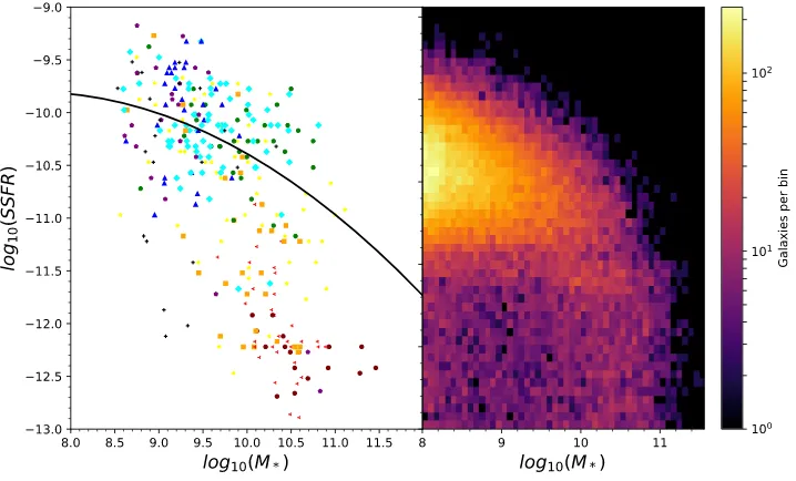
Figure 1. Left:SSFR versus stellar mass for the galaxies in the HRS (E17). The values of SSFR and stellar mass are estimates from the MAGPHYS SED-modelling program (Da Cunha, Charlot & Elbaz2008). The colour and shape of each marker indicate the morphology of the galaxy: maroon circles – E and E/S0; red left-pointing triangles – S0; orange squares – S0a and Sa; yellow stars – Sab and Sb; green octagons – Sbc; cyan diamonds – Sc and Scd; blue triangles – Sd, Sdm; purple pentagons – I, I0, Sm, and Im. The crosses show galaxies for which there is not a clear morphological class (Boselli et al. 2010). The line is a fit to the HRS galaxies with log10(SSFR)>−11.5, which is the region of the diagram covered by late-type galaxies. The line is used in

the Monte Carlo simulation described in Section 4 and has the form log10(SSFR)= −10.39−0.479(log10(M∗)−10.0)−0.098(log10(M∗)−10.0)2. Right:

The artificial sample of 40 000 galaxies generated in the Monte Carlo simulation described in Section 4, plotted in the same diagram as the HRS galaxies.

In this third paper of the series, we step back from trying to make broad inferences about galaxy evolution and consider a detail, albeit an important one. We first investigate where the H-ATLAS galaxies lie on the standard colour versus absolute magnitude plots and whether this distribution differs from the red-sequence/blue-cloud distribution seen for galaxies from an optically selected sample. We then investigate whether the distributions of galaxies in this diagram, whether produced from the SDSS or fromHerschel, can be explained by a continuous, curved GS.

We assume a Hubble constant of 67.3 km s−1_Mpc−1 _{and the} otherPlanckcosmological parameters (Planck Collaboration XXVI 2014).

2 T H E S A M P L E S

For our optical sample, we started from the galaxies detected in the Galaxy and Mass Assembly project (henceforth GAMA). GAMA was a deep spectroscopic survey (Driver et al.2009; Liske et al. 2015) complemented with matched-aperture photometry through-out theUV, optical, and IR wavebands (Driver et al.2016). We used the data from GAMA II (Liske et al.2015), which has a limiting Pet-rosian magnitude ofr<19.8. We used the data from the GAMA9, GAMA12, and GAMA15 fields. The optical sample we use here consists of all the galaxies in these fields with reliable spectroscopic redshifts<0.1 and consists of 20 884 galaxies.

A crucial data product from the GAMA survey that we use in our analysis is estimates of the star formation rates, stellar masses, and dust masses. These were obtained by the GAMA team (Driver et al.2018) by applying the MAGPHYS modelling programme (Da Cunha, Charlot & Elbaz2008) to the matched-aperture photome-try for each galaxy, which extends from theUVto the far-infrared waveband (Wright et al.2016). Very briefly (see Driver et al. for a longer description or the original paper for the full description),

MAGPHYS combines 50 000 possible models of the stellar popu-lation of a galaxy with 50 000 models of dust in the ISM, balancing the energy absorbed by the dust in the optical and UV wavebands with the energy emitted by the dust in the far-infrared, and matches the resultant spectral energy distribution to the observed photome-try. Two of the merits of MAGPHYS are that it makes full use of all the data and that it provides errors on all the parameter estimates. All tests that have been done on the MAGPHYS estimates (seeE17 andE18) suggest that they are robust.

For our submillimetre sample, we started from H-ATLAS. We used the same fields (GAMA9, 12 and 15) that were used to produce the optical sample. The 4σ flux limit of the H-ATLAS survey in these fields is30 mJy at 250μm, the most sensitive wavelength, and there are 113 955 sources above this flux limit (Valiante et al. 2016). The H-ATLAS team used the SDSSr-band images to look for the optical counterparts to these sources, finding 44 835 probable counterparts (Bourne et al. 2016). As our submillimetre sample, we used the 3356 sources in these fields with counterparts with spectroscopic redshifts <0.1. Bourne et al. (2016) estimate that the H-ATLAS counterpart-finding procedure should have found the counterparts to 91.3 per cent of the H-ATLAS sources withz <0.1. Virtually all of these galaxies should have spectroscopic redshifts (Eales et al. 2018). Our sample should therefore be a close-to-complete submillimetre-selected sample of galaxies in the nearby Universe.

Both samples are flux-limited samples, one in the optical wave-band and one in the submillimetre wavewave-band. Both will therefore be subject to Malmquist bias. In the optical sample, optically luminous galaxies will be overrepresented because it is possible to see these to greater distances before they fall below the flux limit of the sam-ple. In the submillimetre sample, galaxies with high submillimetre luminosities will be overrepresented for the same reason.

3 T H E O B S E RV E D C O L O U R D I S T R I B U T I O N S

For both samples, we calculated rest-frame g − r and u − r colours and absoluter-band magnitudes for each galaxy using the GAMA matched-aperture Petrosian magnitudes (Driver et al.2016). In calculating the absolute magnitudes, we used the individualk -corrections for each galaxy calculated by the GAMA team (Loveday et al.2012).

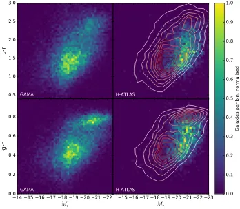
Fig.2shows the distributions of both samples over the colour– absolute magnitude plane. The left-hand panels show the blue cloud and red sequence characteristic of optical samples. Both panels look very similar to the colour–absolute magnitude diagrams in Baldry et al. (2012– their fig. 14), which is not surprising because the two samples are both taken from the GAMA survey and are very similar in the way they were selected.

The right-hand panels show the distributions of the H-ATLAS galaxies. These distributions are quite different from those for the optically selected galaxies, with the peak of the distribution for the submillimetre-selected galaxies shifted in both absolute magnitude and colour from the blue cloud. The colour offset is seen best in the colour distributions in Fig.3. In the left-hand panel, which shows the histograms ofg− r colour, the peak of the distribution for the submillimetre-selected galaxies is in the middle of the green valley. Thus, in the diagram ofg−rcolour versus absolute magni-tude, the submillimetre-selected galaxies form a ‘green mountain’ rather than the red sequence and blue cloud seen for optically se-lected galaxies. The contrast between the optically-sese-lected and submillimetre-selected galaxies is not quite as dramatic foru−r colour, since the peak seen for the submillimetre-selected galaxies is not quite as well centred on the green valley (right-hand panel of Fig.3). However, the distributions for the optically selected and submillimetre-selected samples are still very different, with the dis-tribution for the submillimetre-selected galaxies having a single peak, shifted from the blue cloud to brighter absolute magnitudes and in colour towards the centre of the green valley.

4 M O D E L L I N G T H E D I S T R I B U T I O N S

In this section, we test whether the difference in the colour–absolute magnitude distributions is caused by the different selection effects for optically selected and submillimetre-selected samples. Based on the conclusion from our previous two papers (E17,E18), we start with the assumption that in a diagram of SSFR versus stellar mass, galaxies follow a single, continuous GS rather than a star-forming Galaxy Main Sequence and a separate region of passive galaxies. Therefore, in the modelling in this section, we are also testing whether the idea that there is a single GS is compatible with these very distinctive distributions in the colour–absolute magnitude diagrams.

Before we get into detail, we give a brief overview of our method. There are three stages. In the first stage, we use the GS to generate values of SSFR and stellar mass for an artificial sample of galaxies with redshifts<0.1. The second stage is to associate an optical abso-lute magnitude and colour and a submillimetre luminosity with each artificial galaxy. We do this using the GAMA sample, by finding the GAMA galaxy closest to the artificial galaxy in the SSFR–stellar mass plane, and then assigning the real galaxy’s absolute magni-tude, colour, and submillimetre luminosity to the artificial galaxy. In the third stage, we add the selection effects, finding the subsets of the artificial sample that have flux densities brighter than the optical flux limit (anrmagnitude of 19.8) or the submillimetre flux limit (a flux density of 30 mJy at 250μm).

The aim of the first stage is to create an artificial GS that resembles the empirical GS. The left-hand panel in Fig.1shows the empirical GS from the HRS (E17). The HRS provides a complete inventory of LTGs down to a stellar mass of8×108_M

and of ETGs down to a stellar mass of2×1010_M

(E17). It therefore misses low-mass ETGs, which will fall in the bottom left-hand corner of the figure. However, the total stellar mass of these missing galaxies is quite small;E17estimate that90 per cent of the total stellar mass in ETGs with stellar masses>108_M

is contained in the galaxies actually detected in the HRS. The figure shows that the morpholo-gies of the galaxies gradually change as one moves from the top left to the bottom right of the diagram.E17therefore concluded that galaxies follow a single, curved GS, with galaxy morphology gradually varying along it, rather than there being two separate dis-tributions of star-forming and passive galaxies. The small clump of ETGs at the bottom of the diagram is almost certainly not signifi-cant because estimates of SSFR from SED-fitting programs, such as MAGPHYS and CIGALE, for galaxies with log10(SSFR)<−12.0 are extremely unreliable because the shape of the SED depends so weakly on SSFR in this part of the diagram (Hunt et al. in prepara-tion).

We generated an artificial sample using a GS that resembles the HRS GS in the following way. The first step was to use a random-number generator to generate stellar masses using the stellar mass functions for star-forming galaxies and passive galaxies (Baldry et al.2012) as probability distributions. Baldry et al. divided galaxies into ‘passive’ and ‘star forming’ using a line on the colour–absolute magnitude diagram chosen to separate the red sequence and the blue cloud. We made the approximation that this division is equivalent to a constant value of SSFR,SSFRcut, and used the stellar mass function for star-forming galaxies to generate masses for artificial galaxies for SSFR > SSFRcut and the stellar mass function for passive galaxies to generate masses for artificial galaxies forSSFR< SSFRcut. Note that this is a fairly crude approximation, andE18 showed that galaxies in the red-sequence part of the colour–absolute magnitude diagram extend to quite high values of SSFR (see their fig.5). Given the crudeness of this approximation, we needed a way to tune our model. One possible way would have been to vary the value ofSSFRcut. Instead, for reasons of practicality, we chose a fixed value ofSSFRcut, but used a probability distribution for the stellar masses for galaxies withSSFR<SSFRcut equal to the stellar mass function for passive galaxies multiplied by the parameterfpassive, the one free parameter in our model. In detail, we chose a value forSSFRcut of 10−11 year−1 and used a lower mass limit of 108_M

. We adjustedfpassiveuntil we got roughly the right number of galaxies on the red sequence; we found we got reasonable agreement with a value of 0.5. We discuss the effect of varying this parameter in Section 6.

We assigned a value of SSFR to each galaxy in a differ-ent way depending on whether the galaxy had been assigned to the region below or above SSFRcut. We assumed that the galax-ies with SSFR < SSFRcut are uniformly spread over the range

−13.0<log10(SSFR)<−11.0, using a random-number genera-tor to generate a value for the SSFR of each galaxy. We gener-ated values of SSFR for galaxies with SSFR > SSFRcut in the following way. The upper part of the empirical GS is well fit-ted by a second-order polynomial (Fig. 1, left-hand panel). We used this polynomial to generate values of SSFR for galaxies with SSFR>SSFRcuton the assumption that star-forming galaxies have a Gaussian distribution in log10(SSFR) around this line withσ = 0.5, a value chosen to match the observed spread of the HRS galaxies.

The cause of the green valley/mountain

1187

Figure 2. The distribution of galaxies in the colour versus absoluter-band magnitude plane, with the colour (see the colour scale to the right) showing the density of galaxies in this diagram. The left-hand panels show the GAMA sample and the right-hand panels show the H-ATLAS sample, with the top panels showingu−rcolour versus absolute magnitude and the bottom panels showingg−rversus absolute magnitude. The contours in the right-hand panels show the distributions for the GAMA galaxies that are shown by the colour scale in the left-hand panels.

Figure 3. The distributions ofg−rcolour (left) andu−r(right). The blue (dashed) histogram shows the distribution for the GAMA sample and the green (solid line) histogram the distribution for the sample from H-ATLAS.

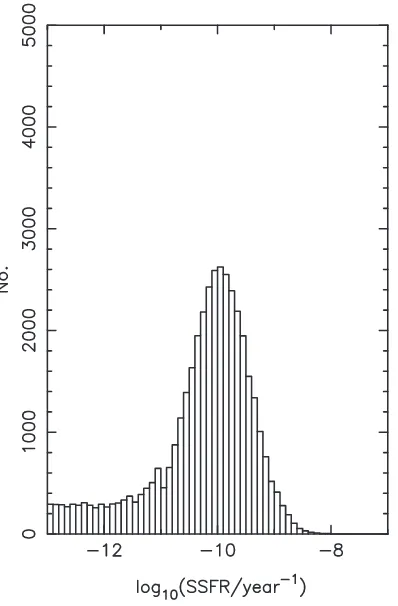
Using this method, we generated values of SSFR and stellar mass for 40 000 galaxies, with the results being shown in the right-hand panel of Fig.1. This procedure generates a smooth, curved GS that looks reasonably like the empirical GS in the left-hand panel. Fig.4shows a histogram of SSFR for the sample, confirming that we have generated a sample of galaxies with a smooth distri-bution in SSFR rather than the bimodal distridistri-bution characteristic

of a separate star-forming main sequence and region of passive galaxies.

There are two important points we wish to emphasize here. The first point is that we do not claim that the GS we are us-ing is a perfect representation of the true GS. The form of this is still poorly known, mainly because of the difficulty of measuring star formation rates in ETGs (E17; Pan et al.2018). The aim of

Figure 4. Histogram of SSFR for the 40 000 galaxies generated in the Monte Carlo simulation described in Section 4.

our modelling is the more modest one of testing whether a con-tinuous GS that looks at least somewhat like the empirical GS shown in the left-hand panel of Fig.1can produce the very distinc-tive distributions in the colour–absolute magnitude diagrams, or whether these distributions can only be produced by galaxies lying in two separate regions of the SSFR versus stellar mass diagram, e.g. a star-forming main sequence and a separate region of passive galaxies.

The second important point is that our division of galaxies into ETGs and LTGs in the first part of our analysis is not part of a circular argument that necessarily produces a red sequence and a blue cloud in the colour–absolute magnitude diagrams. We made this division as part of our procedure for generating a continuous GS and we did not use this division at any future point in the modelling. The division of galaxies into two classes in the first stage of the modelling could only lead to galaxies falling in two separate regions of the colour–absolute magnitude diagrams if it also led to galaxies falling in two separate regions of the SSFR– stellar mass diagrams. Figs1(right-hand panel) and4confirm that this is not the case. Since we have achieved our aim of generating a continuous GS, the division into ETGs and LTGs and all the other details of the first stage of our analysis are now irrelevant and can thankfully be forgotten.

As the final step of the first stage in the modelling, we used a random-number generator to produce a redshift for each galaxy on the assumption that our sample is composed of all the galaxies in a particular region of sky out to a redshift of 0.1.

The second stage is to assign an absolute magnitude, colour, and submillimetre luminosity to each artificial galaxy. We did this by

Figure 5. Luminosity at 250μm versus dust mass for the GAMA galaxies detected withHerschel. The dust masses are the estimates from MAGPHYS (Driver et al.2018).

using the GAMA sample effectively as a look-up table. Each GAMA galaxy has an absolute magnitude, optical colours, and, through the MAGPHYS modelling (Section 2), estimates of SSFR, stellar mass, and dust mass. For the artificial galaxies with log10(SSFR)>−12.0, we found the GAMA galaxy that is closest in the log10(SSFR), log10(M∗) space to the artificial galaxy. Lower values of SSFR have very large errors, and so for artificial galaxies with values of SSFR below this limit, we found the GAMA galaxy that also has log10(SSFR)<−12.0 and that is closest in log10(M_∗) to the artificial galaxy. In both cases, we assigned the absolute magnitude, colours, and MAGPHYS dust mass of the GAMA galaxy to the artificial galaxy.

The one remaining step in this stage is to assign a submillimetre luminosity to each artificial galaxy. We again did this using the GAMA results. Fig. 5shows 250-μm luminosity plotted against the MAGPHYS dust-mass estimate for all the GAMA galaxies that were detected withHerschelat 250μm. The best-fitting line is given by

log10(L250/Watts Hz−1sr−1)=0.87log10(Md/M)+16.3,

with a dispersion in log10(Md) of 0.21. We used this relationship and the MAGPHYS dust mass associated with each artificial galaxy to assign a 250-μm luminosity to each artificial galaxy.

The final stage is to add the selection effects. This is quite easy since each artificial galaxy has an r-band absolute magnitude, a 250-μm luminosity, and a redshift. It is thus simple to calculate the r-band magnitude and the 250-μm flux density of each galaxy, and thus determine which galaxies would be brighter than either the

The cause of the green valley/mountain

1189

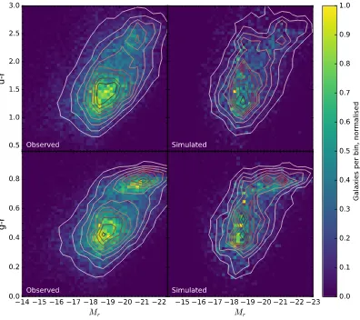
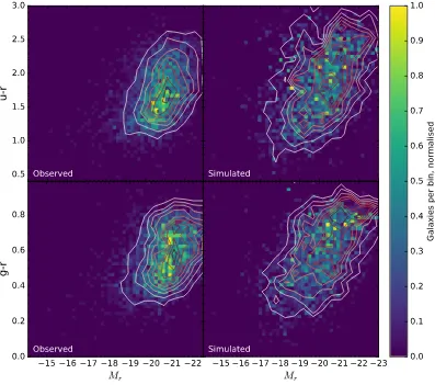
Figure 6. The distribution of galaxies in the colour versusr-band absolute magnitude diagram for the GAMA sample, with the colour showing the density of galaxies in the diagram (see the colour bar to the right). The left-hand panels show the observed distributions, which are the same as shown in the left-hand panels of Fig.2. The right-hand panels show the results of our simulation of where the GAMA galaxies are expected to lie in this diagram if galaxies lie on a continuous, curved GS (Section 4).

GAMAr-band magnitude limit (19.8) or the H-ATLAS 250-μm flux density limit (30 mJy).1

5 R E S U LT S

Of the 40 000 galaxies in the artificial sample, 21 847 have r -band magnitudes<19.8, the magnitude limit for GAMA, and 3646 have 250-μm flux densities>30 mJy, the flux-density limit for H-ATLAS – both fairly similar to the numbers in the real samples. Although the original number of artificial sources was chosen to give roughly the correct number of sources in the real samples, the fact that the ratio of the numbers in the artificial submillimetre and optical samples is similar to the ratio of the numbers in the real samples is circumstantial evidence in favour of our method.

The left-hand panels of Fig. 6 show again the real colour– absolute magnitude distributions for the GAMA sample and the right-hand panels show the distributions for the galaxies in

1_{In carrying out the optical calculation, we used thek-correction from the}

closest GAMA galaxy in the SSFR–M_∗plane. In calculating the 250-μm flux density, we assumed a dust temperature of 20 K.

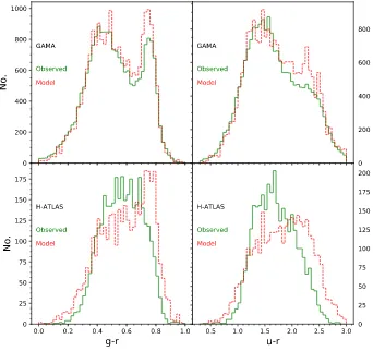
the optically-selected sample of artificial galaxies. Fig. 7shows the same diagram for the observed and artificial submillimetre-selected samples. Fig. 8shows histograms of the colour for the real and artificial optically selected and submillimetre-selected samples.

Let us first consider the results for the optically selected sample. Figs6and8show that our simulation reproduces the qualitative features of the distribution of the galaxies in the colour versus absolute magnitude diagram. It produces a clear red sequence and blue cloud, although it does not produce the quantitative details of the distributions; in particular, there are slightly too many galaxies in the red sequence.

Now let us consider the results for the submillimetre-selected sample, shown in Figs 7and8. Here, the simulation again pro-duces qualitatively the main feature of the observed distribution, since it produces a green mountain shifted in absolute magnitude and colour from the blue cloud for the optically selected galax-ies. However, the quantitative agreement between the predictions and the observations is less good than for the optical sample, since there are too many artificial galaxies on the red side of the green mountain.

Figure 7. The distribution of galaxies in the colour versusr-band absolute magnitude diagram for the H-ATLAS sample, with the colour showing the density of galaxies in the diagram (see the colour bar to the right). The left-hand panels show the observed distributions, which are the same as shown in the right-hand panels of Fig.2. The right-hand panels show the results of our simulation of where the H-ATLAS galaxies are expected to lie in this diagram if galaxies lie on a continuous, curved GS (Section 4).

6 D I S C U S S I O N

The comparison between the predictions and the observations shows that we have achieved our main goal. We have shown that the distinctive features of the distributions of optically-selected and submillimetre-selected galaxies in colour versus absolute magni-tude diagrams can be qualitatively produced from a single, contin-uous GS.

The reader may be concerned that our analysis is circular because of our use of the properties of the GAMA galaxies in the second part of the analysis (Section 4). However, the only use we have made of this sample is to map the transformation between the SSFR/M_∗ space and absolute magnitude–colour space; since the GAMA sam-ple provides good coverage of the former, there is no reason to think that this procedure should introduce any biases.

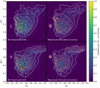
Why does a single, continuous GS produce such very different distributions for an optically selected and a submillimetre-selected sample? We can understand this qualitatively in the following way. First, let us consider the optically selected sample. In the left-hand panels of Fig.9we show the colour–absolute magnitude diagrams for the complete artificial sample of 40 000 galaxies without requir-ing the galaxies to be brighter than ther=19.8 magnitude limit. The red sequence and blue cloud are still apparent, showing the red

se-quence and the blue cloud arenotthe consequence of the magnitude limit but instead the result of the geometric mapping of SSFR/M_∗ to absolute magnitude/colour, which distorts a continuous GS into the distinctive red sequence and blue cloud. As we pointed out in E17, a red sequence is naturally produced because all galaxies with anSSFR<5×10−12_yr−1_{have almost the same colour.}

The right-hand panels of Fig.9show the colour–absolute magni-tude diagrams for the artificial galaxies but with the inclusion again of ther=19.8 magnitude limit and withfpassive, the one free param-eter in our model (Section 4), set to a value of 1.0 rather than 0.5. The appearance of the panels is not very different from the distribu-tions forfpassive=0.5 shown in the right-hand panels of Fig.6, but a plot of the colour histograms shows that increasingfpassiveto 1.0 leads to an increase in the number of galaxies on the red sequence, which is already slightly too high forfpassive=0.5.

Although the implications of this result are profound (see below), it is important to be clear about its limitations. We have shown that the existence of the green valley in plots of colour versus absolute magnitude is not evidence that there are two distinct classes of galaxy (the same is true of plots of the strength of the 4000 Å break versus absolute magnitude – E17), since a green valley is naturally produced even if there is a single, continuous GS in a plot of the intrinsic quantities: SSFR and stellar mass. However,

The cause of the green valley/mountain

1191

Figure 8. Histograms of colour for the GAMA and H-ATLAS samples. In each panel, the green solid line shows the histogram for the real sample and the red dashed line shows the histogram predicted by our simulation based on the assumption of a continuous, curved GS. The left-hand panels showg−rcolour and the right-hand panelsu−rcolour.

we have not proved there is only a single galaxy class because a bimodal distribution of galaxies in the plot of SSFR verses stellar mass would also naturally produce a green valley. The importance of our result is that the existence of the green valley has led to the conclusion that there must be some rapid-quenching process that moves a galaxy rapidly (in cosmic terms) from the blue cloud to the red sequence (Section 1). Our demonstration that the green valley does not imply the existence of two separate distributions of galaxies in the SSFR–stellar mass diagram shows that the discovery of the red sequence sixty years ago was something of a red herring. Let us now turn to the submillimetre-selected sample. By stacking spectra, E18 showed that the red colours of the galaxies in H-ATLAS are not the result of dust reddening but of genuinely old stellar populations. The fact that the green mountain has redder colours than the blue cloud is therefore not the result of theHerschel galaxies containing more dust.

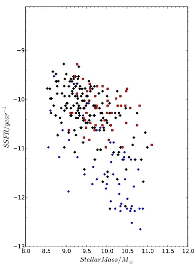
The key diagram that shows the true cause of the green mountain is Fig.10. In this diagram, we plot again the HRS galaxies in the SSFR–M_∗diagram, this time colour coding the points by the ratio of optical-to-submillimetre luminosity for each galaxy. We have calculated this ratio for each galaxy using ther-band magnitudes in Cortese et al. (2012) and the 250-μm flux densities given in Ciesla et al. (2012). For any flux-limited sample, the accessible volume for a galaxy scales roughly as luminosity1.5_{. Therefore, the ratio of} the optical-to-submillimetre luminosity is a measure of the relative Malmquist bias in the two wavebands. For example, if the ratio

was the same for every galaxy, we would expect very similar dis-tributions in the colour versus absolute magnitude diagram for an optically-selected and a submillimetre-selected sample. In Fig.10, the blue points show the 50 galaxies with the highest ratio of optical-to-submillimetre luminosity, the red points the 50 galaxies with the lowest values of this ratio, and the black points the galaxies with intermediate values. The blue points are therefore the galaxies we would expect to see overrepresented in an optically-selected sample and underrepresented in a submillimetre-selected sample, and vice versa. The blue points are mostly massive galaxies with low values of SSFR, which fall on the red sequence in colour–absolute magni-tude diagrams. So it is not surprising that we see a red sequence for an optically selected sample but not for a submillimetre-selected sample. The red points are also fairly massive galaxies but with much higher values of SSFR and are at a position in the diagram where the GS is curving down. The galaxies in this part of the GS will therefore tend to be overrepresented in a submillimetre-selected sample. It is therefore Malmquist bias boosting the representation of this part of the GS that causes the distinctive green mountain in a submillimetre-selected sample. This effect will also lead to these galaxies being underrepresented in an optical sample, deepening the green valley, although the primary reason for the green val-ley is the mapping between SSFR/stellar mass and colour/absolute magnitude.

We can also qualitatively explain why the difference in colour between the Herschel-selected galaxies and the blue cloud is

Figure 9. The distribution of galaxies in the colour versus absolute magnitude diagram, with the colour showing the density of galaxies in this diagram (see the colour scale to the right). The left-hand panels show the distribution for all 40 000 galaxies in our artificial sample (Section 4) when no flux limit is imposed on the sample. The right-hand panels show the result for an artificial sample withfpass, the multiplicative factor for the stellar mass function of passive galaxies

(Section 4), set to 1, for the artificial galaxies that satisfy the GAMA magnitude limit (r<19.8). To see the effect of changing the value of this parameter, these panels should be compared with the right-hand panels of Fig.6, for whichfpass=0.5.

greater for g − r than for u − r (Fig. 3). The stacked spec-tra in E18 show that the Herschel-selected galaxies have both a significant 4000 Å break, indicating an old stellar population, and an upturn in theUV part of the spectrum, indicating large numbers of young stars. The g − r colours will be more sen-sitive to the old stellar population, dragging the colour distribu-tion for theHerschelgalaxies towards the red sequence; theu− rcolours will be more sensitive to theUVemission from young stars, pulling the colour distribution towards the star-forming blue cloud.

Our result removes the most obvious evidence for rapid quench-ing in the galaxy population. There are a number of other recent studies, using a variety of methods, that have also investigated whether rapid quenching is an important part of galaxy evolution. Casado et al. (2015) used a comparison of estimates of the recent star formation rate in galaxies with star formation estimates for the same galaxies at an earlier time to show that there is no evi-dence of a rapid-quenching process in low-density environments, although there is evidence for this in dense environments. Using a similar technique, Schawinski et al. (2014) found evidence for slow quenching in LTGs but rapid quenching in ETGs. Peng, Maiolino & Cochrane (2015) used the metallicity distributions of star-forming and passive galaxies to argue that the evolution from one population to the other must have occurred over4 billion yr – slow quenching. Schreiber et al. (2016) concluded that at high redshift the decrease

in the slope of the star-forming main sequence at high stellar masses can be explained by slow quenching. Although the same problem of measuring accurate values for SSFR at low values of SSFR exists at high redshift, the best evidence for galaxies lying in two distinct regions of the SSFR–stellar mass diagram comes from high-redshift samples (Elbaz et al. 2017 – their fig. 17; Magnelli et al.2014– their fig. 2).

Finally, a couple of very recent studies have investigated directly the evolution of the galaxies in the green-valley part of the colour– absolute magnitude diagram. Bremer et al. (2018) used the colours and structures of the galaxies in the green valley to show that galax-ies are evolving slowly across this region. A follow-up study by Kelvin et al. (2018) has used the structures of the green-valley galaxies to show that the transition across this region does not re-quire a rapid-quenching process. Our results nicely explain these two results, since if the green valley is an artefact of the geomet-ric transformation from intrinsic to observed quantities, there is no reason to expect galaxies in this part of the diagram to be evolving quickly.

One possible way to reconcile all of the results above, as we ar-gued inE17, would be if most galaxies evolve by gradual processes (slow quenching) with the 14 per cent of ETGs that are slow rota-tors (Cappellari et al.2013) being produced by a rapid-quenching process.

The cause of the green valley/mountain

1193

Figure 10. The distribution of the HRS galaxies in the SSFR–M_∗plane with the points coloured to show the ratio of optical (rband) to submil-limetre (250μm) luminosity for each galaxy. The blue circles show the 50 galaxies with the highest ratios of optical-to-submillimetre luminosity, the red squares show the 50 galaxies with the lowest ratios of optical-to-submillimetre luminosity, and the black diamonds the other HRS galaxies.

7 C O N C L U S I O N S

We have shown that the galaxies found in a sample selected at submillimetre wavelengths have a very different distribution in a colour–absolute magnitude diagram than galaxies selected at op-tical wavelengths. Whereas the opop-tically selected galaxies form a red sequence and a blue cloud with a green valley in between, a submillimetre-selected sample forms a green mountain.

We have shown that we can reproduce the qualitative features of both distributions if galaxies lie on a single, curved, continuous GS in a plot of SSFR versus stellar mass. The main cause of the red sequence and the blue cloud is the geometric mapping between stellar mass/SSFR and absolute magnitude/colour, which distorts a continuous GS in the diagram of intrinsic properties into a bimodal distribution in the diagram of observed properties. The cause of the green mountain is Malmquist bias in the submillimetre waveband, which causes galaxies on the curved part of the GS to be overrep-resented in a submillimetre sample. This effect, working in reverse, causes galaxies on this part of the GS to be underrepresented in an optical sample, deepening the green valley.

The existence of the green valley for an optical sample is therefore not evidence (1) for there being two distinct populations of galaxies, (2) for galaxies in this region evolving more rapidly than those in the blue cloud and red sequence, and (3) for rapid-quenching processes in the galaxy population.

AC K N OW L E D G E M E N T S

We thank the many scientists who have contributed to the success of theHerschelATLAS and the HRS. We are also grateful to Leslie Hunt for useful conversations about the relative strengths and

lim-itations of the SED-fitting programs MAGPHYS, CIGALE, and GRASIL and for making available a draft of her paper on the sub-ject. This research made use of Astropy, a community-developed core Python package for Astronomy (Astropy Collaboration2013), and Matplotlib, a Python 2D plotting library (Hunter2007). EV and SAE acknowledge funding from the UK Science and Tech-nology Facilities Council consolidated grant ST/K000926/1. MS and SAE have received funding from the European Union Seventh Framework Programme ([FP7/2007-2013] [FP7/2007-2011]) under grant agreement no. 607254. LD and SM acknowledge support from the European Research Council (ERC) in the form of Consolida-tor GrantCOSMICDUST(ERC-2014-CoG-647939; PI: H L Gomez). LD, SJM, and RJI acknowledge support from the ERC in the form of the Advanced Investigator Program, COSMICISM (ERC-2012-ADG 20120216; PI: R.J.Ivison). MJM acknowledges the support of the National Science Centre, Poland through the POLONEZ grant 2015/19/P/ST9/04010.

R E F E R E N C E S

Astropy Collaboration, 2013, A&A, 558, 33 Baldry I. K. et al., 2012,MNRAS, 441, 2440 Baum W. A., 1959,PASP, 71, 106

Bell E. R., McIntosh D. H., Katz N., Weinberg M. D., 2003,ApJS, 149, 289 Boselli A., Gavazz G., 2006,PASP, 118, 517

Boselli A. et al., 2010,PASP, 122, 261

Bournaud F., Elmgreen B. G., Elmgreen D. M., 2007,ApJ, 670, 237 Bourne N. et al., 2016,MNRAS, 462, 1714

Bremer M. N. et al., 2018,MNRAS, 476, 12 Cappellari M. et al., 2013,MNRAS, 432, 1862

Casado J., Acasibar Y., Gavilan M., Terlevich R., Terlevich E., Hoyos C., Diaz A. I., 2015,MNRAS, 451, 888

Cicone C. et al., 2014,A&A, 562, A21 Ciesla L. et al., 2012,A&A, 543, A161 Clark C. J. R. et al., 2015,MNRAS, 452, 397 Cortese L., 2012, A&A, 543, 101

Cortese L. et al., 2012,A&A, 544, A101 Cortese L. et al., 2016,MNRAS, 463, 170

Da Cunha E., Charlot S., Elbaz D., 2008,MNRAS, 388, 1595 Daddi E. et al., 2007,ApJ, 670, 156

Driver S. et al., 2009,Astron. Geophys., 50, 12 Driver S. et al., 2016,ApJ, 827, 108

Driver S. et al., 2018,MNRAS, 475, 2891 Eales S. et al., 2010,PASP, 122, 499

Eales S., de Vis P., Smith M. W. L., Appah K., Ciesla L., Duffield C., Schofield S., 2017,MNRAS, 465, 3125 ( E17)

Eales S. et al., 2018,MNRAS, 473, 3507 ( E18) Elbaz D. et al., 2007,A&A, 468, 33

Emsellem E. et al., 2011,MNRAS, 414, 888 Furlanetto C. et al., 2018,MNRAS, 476, 961 Gavazzi G. et al., 2015,A&A, 580, A116 Genzel R. et al., 2011,ApJ, 733, 101 Genzel R. et al., 2014,ApJ, 785, 75 Hunter J. D., 2007, Comput. Sci. Eng., 9, 90 Kelvin L. et al., 2018,MNRAS, 477, 4116 Lee N. et al., 2015,ApJ, 801, 80 Liske J. et al., 2015,MNRAS, 452, 2087 Loveday J. et al., 2012,MNRAS, 420, 1239 Maddox S. et al., 2018,ApJS, 236, 30 Magnelli B. et al., 2014,A&A, 561, A86

Martig M., Bournaud F., Teyssier R., Dekel A., 2009,ApJ, 707, 250 Noeske K. G. et al., 2007,ApJ, 660, L43

Noguchi M., 1999,ApJ, 514, 77

Oemler A., Abramson L. E., Gladders M. D., Dressler A., Poggianti B. M., Vulcani B., 2017,ApJ, 844, 45

Pan H.-A. et al., 2018,ApJ, 854, 159

Peng Y., Maiolino R., Cochrane R., 2015,Nature, 521, 192 Peng Y.-J. et al., 2010,ApJ, 721, 193

Pilbratt G. et al., 2010,A&A, 518, L1

Planck Collaboration XXVI, 2014,A&A, 571, A26 Rodighiero G. et al., 2011,ApJ, 739, L40 Schawinski K. et al., 2014,MNRAS, 440, 889

Schreiber C., Elbaz D., Pannella M., Ciesla L., Wang T., Koekemoer A., Rafelski M., Daddi E., 2016,A&A, 589, A35

Smith M. W. L. et al., 2017,ApJS, 233, 26 Strateva I. et al., 2001,AJ, 122, 1861 Tomczak A. et al., 2016,ApJ, 817, 118

Toomre A., 1977, in Tinsley B. M. Larson R. B., eds, Evolution of Galaxies and Stellar Populations, Proceedings of a Conference at Yale University. Yale University Observatory, New Haven, Conn., p. 401

Valiante E. et al., 2016,MNRAS, 562, 3146 Visvanathan N., 1981,A&A, 100, L20 Whitaker K. et al., 2014,ApJ, 795, 104 Wright A. et al., 2016,MNRAS, 460, 765

1_{School of Physics and Astronomy, Cardiff University, The Parade, Cardiff}

CF24 3AA, UK

2_{Sterrenkundig Observatorium, Universiteit Gent, Krijgslaan 281 S9,}

B-9000 Gent, Belgium

3_{Institute for Astronomy, The University of Edinburgh, Royal Observatory,}

Blackford Hill, Edinburgh EH9 3HJ, UK

4_{Astrophysics Group, Department of Physics, University of Bristol, Tyndall}

Avenue, Bristol BS8 1TL, UK

5_{School of Physics and Astronomy, Monash University, Clayton, Victoria}

3800, Australia

6_{Astrophysics Group, Imperial College London, Blackett Laboratory, Prince}

Consort Road, London SW7 2AZ, UK

7_{Institut d’Astrophysique Spatiale, CNRS, Universit´e Paris-Sud, Universit´e}

Paris-Saclay, Bat. 121, F-91405 Orsay Cedex, France

8_{International Centre for Radio Astronomy Research, 7 Fairway, The}

Uni-versity of Western Australia, Crawley, Perth, WA 6009, Australia

9_{School of Physics and Astronomy, University of Nottingham, University}

Park, Nottingham NG7 2RD, UK

10_{Instituto de F´ısica, Universidade Federal do Rio Grande do Sul, Av. Bento}

Gonc¸alves, 9500, 91501-970 Porto Alegre, RS, Brazil

11_{Department of Physics and Astronomy, 102 Natural Science Building,}

University of Louisville, Louisville, KY 40292, USA

12_{European Southern Observatory, Karl-Schwarzschild-Strasse 2, D-85748}

Garching, Germany

13_{Astrophysics Research Institute, Liverpool John Moores University, 146}

Brownlow Hill, Liverpool L3 5RF, UK

14_{Dark Cosmology Centre, Niels Bohr Institute, University of Copenhagen,}

Juliane Maries Vej 30, DK-2100 Copenhagen, Denmark

15_{College of Graduate Studies, University of South Africa, PO Box 392,}

UNISA, 0003, South Africa

16_{Astronomy Centre, University of Sussex, Falmer, Brighton BN1 9QH, UK} 17_{Faculty of Physics, Astronomical Observatory Institute, Adam Mickiewicz}

University, ul. Słoneczna 36, PL-60-286 Pozna´n, Poland

18_{Centre for Astrophysics Research, School of Physics, Astronomy and}

Mathematics, University of Hertfordshire, College Lane, Hatfield AL10 9AB, UK

19_{Leiden Observatory, PO Box 9513, NL-2300 RA Leiden, the Netherlands} 20_{Argelander-Institut fur Astronomie, Auf dem Hugel 71, D-53121 Bonn,}

Germany

This paper has been typeset from a TEX/LA_{TEX file prepared by the author.}