Automated Bilateral Bargaining about Multiple Attributes in a One to Many Setting

(1)

Automated Bilateral Bargaining about Multiple Attributes

in a One-to-Many Setting

E.H. Gerding

Center for Mathematics and Computer Science(CWI) P.O. Box 94079, 1090 GB Amsterdam, The Netherlands

D.J.A. Somefun

Center for Mathematics and Computer Science(CWI) P.O. Box 94079, 1090 GB Amsterdam, The Netherlands

J.A. La Poutr´e

Center for Mathematics and Computer Science(CWI) and Technical Univ. Eindhoven School of Techn. Management

P.O. Box 513, 5600 MB Eindhoven, The Netherlands

ABSTRACT

Negotiations are an important way of reaching agreements between selfish autonomous agents. In this paper we fo-cus on one-to-many bargaining within the context of agent-mediated electronic commerce. We consider an approach where a seller agent negotiates over multiple interdependent attributes with many buyer agents in a bilateral fashion. In this setting, “fairness,” which corresponds to the notion of envy-freeness in auctions, may be an important business constraint. For the case of virtually unlimited supply (such as information goods), we present a number of one-to-many bargaining strategies for the seller agent, which take into account the fairness constraint, and consider multiple at-tributes simultaneously. We compare the performance of the bargaining strategies using an evolutionary simulation, especially for the case of impatient buyers. Several of the developed strategies are able to extract almost all the sur-plus; they utilize the fact that the setting is one-to-many, even though bargaining is bilateral.

1. INTRODUCTION

From a business perspective electronic markets have the potential danger of becoming increasingly more transpar-ent with low search cost, strong price competition, and low margins. Automated negotiation enables a business to go beyond price competition. Through the use of autonomous agents, which negotiate on behalf of their owners, a busi-ness can obtain flexibility in prices and goods, distinguish between groups of buyers based on their preferences, and even personalize complex goods according to the demands of individual buyers without significantly increasing trans-action costs.

It is common to characterize negotiations by their setting:

bilateral, one-to-many, or many-to-many. We focus on the one-to-many bargaining setting in this paper, where a seller agent negotiates, on behalf of a seller, with many buyers individually in a bilateral fashion. In this paper we develop various strategies for this setting which enable a seller agent to bargain over multiple interdependent issues simultane-ously and effectively.

In many cases, auctions can be used to effectively organize one-to-many bargaining. Depending on the setting, auc-tions can provide buyers with the incentive to reveal their preferences truthfully, and to allocate the goods efficiently. For various situations, however, auctions may not be the preferred protocol for bargainers. In situations of, for ex-ample, virtually unlimited supply, multiple issues, and/or continuous sale the appropriate auction protocol becomes, at best, much more complex. Consequently, businesses may opt for the intuitive and flexible bilateral bargaining proto-col, where the seller agent negotiates bilaterally with one or more buyers simultaneously by exchanging offers and counter offers.

In many electronic commerce domains the supply is flexi-ble and new goods can be reproduced quickly, at relatively low costs. This is especially the case for information goods, where the reproduction costs are almost zero, but it may also be the case in other retail markets. With virtually unlim-ited supply, there is no direct competition between buyers. In that case, auctions such as the standard Vickrey auction fail to provide sufficient profit for the seller (cf., for exam-ple, [1] for a possible solution). Secondly, bargaining can also naturally include more complex goods, where not just the price is negotiated, but many other issues as well, such as service, quantity, quality, and warranty. Especially with a relative large number of issues (cf. [9]) and flexible supply a myriad of bargaining outcomes are possible; consequently, even with many buyers, bargaining is really bilateral. With many buyers, a seller may however still utilize the one-to-many setting to determine and adjust the utility level of an offer. Thirdly, bargaining can be easily applied in case of continuous sales. Auctions usually end or even start at a fixed point in time.1

Using bargaining, new buyers can

en-1

The double auction used in certain financial markets with many-to-many negotiation is an example of a continuous Permission to make digital or hard copies of all or part of this work for

(2)

ter the negotiation at any given time, and buyers can obtain the good at any time by accepting a seller’s counter offer.

Potentially, bargaining can lead to unsatisfied customers if buyers perceive the outcomes of the negotiations as unfair. This can occur when, for instance, two customers obtain similar goods at the same time but end up paying very differ-ent amounts. Fairness of negotiation outcomes is important for customer satisfaction, which in turn may be important for a business’ long term profitability. The seller agent can prevent unfair outcomes by incorporating a fairness norm, comparable to the notion of envy-freeness in auctions [8], whereby customers are treated in a similar fashion. This fairness aspect emphasizes that bargaining is really one-to-many.

For the case of virtually unlimited supply, as for informa-tion goods, we present a number of one-to-many bargaining strategies for the seller in this paper, which take into account the fairness constraint and bargain over multiple attributes. We compare the performance of the bargaining strategies using an evolutionary simulation, especially for the case of impatient buyers. One set of strategies, the so-called “re-sponsive threshold” strategies, are able to extract almost all the surplus, given sufficient time pressure. These strategies benefit from the fact that the setting is one-to-many, even though bargaining occurs in a bilateral fashion. In addition, the strategies are able to find win-win agreements (i.e., very little Pareto improvement is possible).

A number of related papers study bargaining using an evo-lutionary approach, e.g. [7, 6, 11, 3]. Our approach extends previous research to multiple (types of) buyers and bilateral negotiation strategies for one-to-many multi-issue bargain-ing which can benefit from time pressure.

In addition a growing body of literature exists on multi-issue negotiation, which focus on developing techniques a seller and/or a buyer can use to determine the relative magnitude of the various issues and consequently search for approxi-mately win-win (or Pareto-efficient) deals [9, 5, 4, 10, 13]. Although we also consider the problem of how to determine the values for the various attributes of an offer, the focus of the paper lies on the development of “threshold” strategies for one-to-many negotiation. These strategies determine the desired utility level of a deal and can be used in conjunction with the techniques already developed in the literature.

The remainder of the paper is organized as follows. In Section 2 we describe the bargaining setting and introduce strategies for one-to-many bargaining. In Section 3 we dis-cuss the simulation environment used for testing the perfor-mance of the strategies. We present the simulation results of the conducted computer experiments in Section 4. Con-clusions follow in Section 5.

2. ONE-TO-MANY BARGAINING

2.1 Fairness

An agent representing a business can be endowed with var-ious bargaining strategies. The bargaining outcome should,

auction; these markets are however characterized by limited supply.

however, be fair. Because fairness must be ensured by the seller and because buyer preferences are private, we define fairness as follows. Suppose at time td a buyer reaches a

deal. We say that this deal is fair, relative to a fixed in-terval ∆ > 0, whenever there exist a start time ts, with

td ∈[ts, ts+ ∆], such that the seller is indifferent between

any other deal reached within the interval [ts, ts+∆].

When-ever price is the only issue, a buyer does not strictly prefer any deal for which the seller is indifferent. In this case, we can give the following equivalent definition: a deal is fair, relative to a fixed interval ∆ > 0, whenever there exist a start timets, withtd∈[ts, ts+ ∆], such that the buyer does

not strictly prefer any other deal which is reached within the interval [ts, ts+ ∆]. Note, that this definition of fairness

is closely related to the notion of envy-free auctions in [8]; it adapts the notion of envy-freeness to the more continuous setting of bilateral bargaining.

2.2 Bargaining Protocol

The seller agent negotiates with many buyer agents simul-taneously in a bilateral fashion by alternating offers and counter offers. An offer specifies a value for each attribute of the negotiation, such as the price, quality, quantity, and other relevant aspects. The protocol allows for multiple

offers to be submitted simultaneously. Exchanging multi-ple offers can improve the (Pareto) efficiency of agreements made when several attributes are concerned. An offer con-stitutes a Pareto improvement over another offer whenever it makes one bargainer better off without making the other worse off. A bargainer proposing multiple offers can be indif-ferent between those offers whereas his opponent may prefer a particular offer and can improve efficiency by selecting this offer.

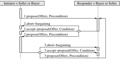
We call the set of offers combined with the preconditions a proposal. A bargainer can accept one of the submitted offers or reject all offers and place a counter proposal. Ne-gotiations between a buyer and seller agent proceed to the next round whenever a proposal is submitted and terminates when one of the submitted offers is accepted or after a prede-fined period of time has elapsed. Note that a bargainer can introduce a delay before submitting a counter proposal. The duration of a round varies depending on the delay. Figure 1 depicts the alternating offer bargaining protocol.

Responder = Buyer or Seller Initiator = Seller or Buyer

1:propose(Offers, Precondition)

2:abort−bargaining

2:accept−proposal(Offer, Condition) 2:propose(Offers, Precondition)

3:accept−proposal(Offer, Condition) 3:abort−bargaining

[image:2.595.318.557.525.645.2]

3:propose(Offers, Precondition)

Figure 1: The agents’ bargaining protocol

2.3 Time Pressure

(3)

impa-tience is a common assumption in bargaining, e.g. [12]. The seller agent is simultaneously and continuously negotiating with many buyers and is therefore less concerned with im-mediately reaching an agreement for a particular bargaining outcome, i.e., he is relatively patient. We model this relative time patience by assuming that the seller, unlike the buyers, has no time pressure.

At least in theory, the seller can benefit from buyers’ time-pressure by introducing a delay before submitting a counter proposal. An important question is then which bargaining strategies can most effectively utilize these potential bene-fits. Experimental results discussed in Section 4 show that responsive threshold strategies, which we will discuss in the next Section, are very effective: depending on the time pres-sure, they are capable of extracting very large shares of the seller surplus. (Reasoned from the seller’s perspective the surplus is just the maximum utility he can realize by selling the goods or services.)

2.4 One-to-Many Bargaining Strategies

The challenge is to develop bargaining strategies for the seller agent that maximize overall revenue by utilizing dif-ferences in buyers’ willingness to pay without violating the fairness constraint. Instead, these strategies utilize differ-ences indirectly through buyers’ time pressure. In order to benefit from time pressure, a strategy specifies, in addition to an actual (counter) proposal or an acceptance proposal, when to respond to an opponent’s proposal.

The seller strategies as developed determine the offers of a proposal in two steps. First, they specify a threshold level which sets the utility level of the offers. Second, they gener-ate the values for the individual attributes, given the thresh-old. Advanced techniques for multi-issue negotiation, as for instance discussed in [9, 5, 4, 10, 13], can be applied to the latter. The focus of this paper is on effective strategies for determining the threshold, and we therefore only consider the relatively simple technique of randomly determining the attribute-values given a threshold. The probability with which a value of an attribute is determined may however depend on a buyer’s corresponding offer (see below).

Besides specifying the utility of a (counter) proposal, the threshold is also used to determine when to respond to an outstanding proposal. More precisely, a seller strategy re-sponds with a fixed delay to all outstanding proposals which lie below the (current) threshold value; a proposal lies be-low the threshold value whenever the seller’s utility for all offers in the proposal lies below the threshold value. While applying a delay to all proposals below the threshold value, the seller agent continues to negotiate with the remaining buyers by immediately responding with a counter proposal.

This negotiation without delay with the select group of buy-ers can, in principle, continue for several rounds. During these rounds the threshold is not adjusted. The goal at this time is to improve the Pareto-efficiency of the final agreement by finding mutually beneficial trade offs between the various attributes. In the simulation the seller agent only makes a single proposal to improve the efficiency of the deal. For a particular proposal of a buyer the seller strat-egy randomly generates offers within the neighborhood of

the buyer’s best offers, i.e., with the highest utility for the seller. This already suffices for very efficient outcomes. If a buyer does not accept one of the seller agent’s offers, the seller agent will again respond with a delay.

Another aspect that needs to be considered by the seller agent is the fairness of the agreements. Fairness prescribes that the seller should be indifferent between the deals made within the defined time interval. Whenever the seller agent almost simultaneously accepts two different offers a bargain-ing outcome may be unfair. The seller strategy ensures fair-ness by always making a (interesting) counter proposal, in-stead of accepting an offer directly.

The seller agent can be equipped with a number of strategies for determining the threshold, which we introduce below.

2.4.1 Fixed & Time-Dependent Threshold Strategies

For purpose of comparison we introduce a fixed threshold strategy. Clearly, the fixed threshold strategy is not capable of utilizing buyers’ time pressure. The purpose of the strat-egy is to provide some insights in the minimal extractable profit, given strategic behavior of the buyers.

The second strategy we consider is a time-dependent thresh-old strategy: the current utility or threshthresh-old depends on time. The threshold only changes from one period to the next. Unlike the fixed-threshold strategy the time-dependent strategy is capable of utilizing buyers’ time pres-sure. Its success, however, depends on how much it knows about buyers’ preferences, or how easily more about buyers’ preferences can be learned, in relation to time-based pricing strategies.

2.4.2 Responsive Threshold Strategies

The fixed and time-dependent threshold strategies do not adjust the threshold based on the buyers’ offers. Inspired by the first-price auction, we introduce another type of bargain-ing strategy with a responsive threshold. With this strategy, all offers submitted by the buyers within a certain fixed time interval are collected after the previous offers made by the seller agent. Then it determines thecurrent highest utility, which is equal to the utility of the best offer from the col-lection of offers. The threshold is set to the current highest utility.

(4)

other ongoing negotiations. The point is that unlike a true auction the relationship with other simultaneously submit-ted offers is not specified up front, through a set of rules.

Reservation ValueA drawback of the responsive thresh-old strategy is that it becomes vulnerable whenever groups of buyers experience very little time pressure. Without time pressure buyers have no incentive to buy soon. They may all independently decide to initially submit very low offers; consequently utility will be very low for the seller. To cir-cumvent this we also consider responsive threshold strategies with a reservation value. A seller agent is never willing to sell below the reservation value. This means we alter the earlier definition of the current highest utility. It now be-comes the maximum of the reservation value and the best offer from the offers collected within a certain time interval. An interesting advantages of introducing a reservation value occurs when some but not all buyers experience very little time-pressure. The responsive threshold strategy can then still utilize the time-pressure of the other buyers.

We consider two approaches for determining the reservation value. Either the reservation value is fixed, like the fixed-threshold strategy, or it is time dependent, like the time-dependent threshold strategy. Thus the responsive thresh-old strategy with a reservation value is actually a combina-tion of the responsive threshold strategy (without reserva-tion value) and either the fixed or time-dependent strate-gies.

3. SIMULATION ENVIRONMENT

We apply a simulation environment in order to evaluate the performance and robustness of the above negotiation strate-gies against many learning buyers. The agents in the simu-lation are assumed to be boundedly rational: they can learn and adapt their strategies by a process of trial and error, and they do not know the seller’s strategy. The bargaining pro-cess is repeated many times, enabling buyers and the seller to learn from past interactions. An evolutionary algorithm is used to model the learning aspect of the agents. This is a common approach within the field of agent-based compu-tational economics (ACE) [14]. A number of related papers study bargaining using an evolutionary approach, e.g. [7, 6, 11, 3]. Our approach extends previous research to multi-ple (types of) buyers and bilateral negotiation strategies for one-to-many multi-issue bargaining which can benefit from time pressure.

3.1 The Bargaining Game

The seller agent negotiates with many buyer agents simulta-neously by alternating offers and counter offers as described in Section 2.2, where the buyer agents initiate the nego-tiations. For our simulations we set a maximum number ofn discrete periods, where n is set sufficiently large such that it has no significant impact on the results. For the analysis we assume that offers consist of two interdependent attributes, e.g. the price and the quality. We note that buyer agents in the simulation do not leave the negotiations or enter later. We also assume that, since buyers are im-patient, buyer agents in the simulation will respond to the seller agent’s counter offers without delay. This is modeled by having the buyer’s counter proposal or acceptance pro-posal occur in the same period as the seller’s propro-posal.

3.2 Buyers and their Agents

Buyers are interested in buying at most one good in each bargaining game. They can have different preferences re-garding the time pressure and attribute value combinations, which together constitute the buyer type. For the analysis we assume a finite number ofktypes. Althoughk is fixed, the number of participating buyer agents of each type varies randomly for each negotiation game and is determined in-dependently by a Poisson distribution with averagem.

To illustrate the feasibility of our approach for interdepen-dent attributes, we use the well-known Cobb-Douglas utility function to represent a player’s preferences for the two at-tributes. More specifically, the utilityui for buyer typeiin

case of a disagreement equals zero and in case of an agree-mentuiis defined as

ui= (v1,i−o1)

αi₍

v2,i−o2)

βi

δti,

where αi and βi are parameters that indicate the relative

importance of the attributes, o1 ando2 are the negotiated

values the seller receives for the attributes (and the buyer has to give in), and v1,i and v2,i represent the maximum

buyer i’s is willing to give in on the individual attributes. For example, let attribute 1 and 2 refer to price and quality. Then o1 represents the price ando2 the difference between

the maximum quality and the actual quality of the good received;v1,i then represents the maximum price buyeriis

willing to pay and v2,i the maximum buyer i is willing to

give in on the quality. Furthermore,δiis the discount factor

used to model the time pressure, and t is the negotiation time. In the simulation depreciation occurs at discrete time intervals. Therefore,δiis the discrete representation of time

pressure and tindicates the period in which an agreement is reached. Note that discount factors are commonly used for modeling time pressure, e.g. in the Rubinstein-St˚ahl alternating-offers model [12].

3.2.1 Buyer Agent’s Strategy

The buyer agents in the simulation apply time-dependent strategies similar to the seller’s time-dependent threshold strategy described in Section 2.4. The buyer agent uses a strategy similar to the random strategy of the seller (see Section 2.4) to determine the values of the attributes, given the threshold. The time-dependent strategy consists of a piece-wise linear function to determine the threshold. The parameters that determine the function are adaptive: using an evolutionary algorithm they evolve such that the perfor-mance of the strategy increases.

We also applied an extended strategy in our experiments by using two separate piece-wise linear functions: one produces the threshold for determining the utility level of the offers and the other function determines the threshold for accept-ing or rejectaccept-ing the seller’s offers. The separation of the two functions enhances the bargaining capabilities of the buyer agent. Results using the two representations are very simi-lar. The outcomes presented in this paper are based on the extended strategy.

3.3 Seller Agent

(5)

selection

parents

offspring

selection reproduction

reproduction

parents

offspring

parents offspring

negotiation game

buyer type 1 buyer type 2

seller selection

[image:5.595.75.272.51.244.2]

reproduction

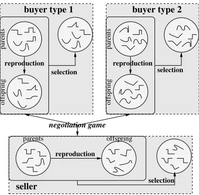
Figure 2: The EA cycle for negotiations with two buyer types and an adaptive seller

agent’s utility in case of an agreement equalsus=oα1so βs

2 ,

and is zero in case of a disagreement (recall from Section 2.3 that we can assume that the seller has no time pressure). The total utility equals the sum of utilities obtained over all buyers. Production costs are set to zero.

We consider five strategies for the seller agent: fixed thresh-old, time-based threshthresh-old, responsive threshold and two combined strategies (see also Section 2.4). The time-based threshold strategy is similar to the strategy used by the buyer. The first two strategies and the combined strategies have parameters which determine respectively the threshold value and the reservation value during a bargaining game. These parameters areadaptive: optimal values are learned using an evolutionary algorithm, explained below. The re-sponsive threshold strategy does not have any parameters that need to be learned.

3.4 The Evolutionary Algorithm

Evolutionary algorithms (EAs) are a class of search algo-rithms inspired by Darwin’s theory on variation and natural selection, and are becoming increasingly popular for model-ing economic behavior, particularly within the field of agent-based computational economics (ACE), see e.g. [14]. We use an implementation based on “evolution strategies” [2], which is typical for real-valued encoding of the strategies (whereas the more popular branch of “genetic algorithms” is originally based on binary encoding).

The EAs are used to produce effective bargaining strategies for the buyer agents. Strategies for the agents of different buyertypesare produced by separate EAs, which operate in parallel. This allows for heterogeneous strategies to emerge. Furthermore, in case of an adaptive seller agent, a separate EA is also used to produce strategies for the seller agent. A graphical representation of the evolutionary simulation with two buyer types and an adaptive seller agent is given in Fig. 2.

Each EA starts with a population ofparentstrategies, which are randomly generated. The EA then performs the follow-ing cycle to improve the quality orfitnessof the strategies. First, the reproduction operator generates a population of

offspring strategies by randomly selecting strategies from the parent population and slightly mutating the strategy to obtain variation.

In the next step, the fitness of the strategies is determined by the average utility obtained in a number of bargaining games. At the start of each bargaining game, the number of participating buyers of each type is determined randomly us-ing a Poisson distribution as described above. Buyer agents are then generated for each buyer and are assigned a ran-domly selected strategy from either the parent or offspring population of the corresponding type. Similarly, a strat-egy is selected randomly for the seller agent (in case of an adaptive seller). The bargaining game is played for a fixed number of times, determining the number of buyers and as-signing new strategies at the start of each game.

In the final stage of the cycle, a deterministic selection scheme called (µ+λ)-selection chooses the strategies with the highest fitness from both the parents and the offspring populations as the new parents for the next generation [2]. The cycle is repeated for a fixed number of generations.

3.4.1 Strategy encoding

As mentioned in Section 3.2, the buyer agent’s strategy con-sists of two piece-wise linear functions: an offer and a thresh-old function. The functions are encoded using real values, where each bending point of a function is encoded by two real values (i.e., the period and the corresponding threshold value). Additionally, two end points mark the values for the first and last period. For example, 8 real values are needed to encode a pair of functions with two line pieces each.

The same representation is used for the seller agent if he uses a time-based threshold strategy. If a fixed threshold is used, only a single real value is needed to encode this. Note that the seller agent uses the same function for both the threshold and for producing offers.

3.4.2 Mutation with Exponential Decay

The mutation operator changes the strategy of an agent as follows. Each real value xi is mutated by adding a

zero-mean Gaussian variable with a standard deviation σ [2]:

x0

i:=xi+σNi(0,1). All resulting values larger than unity

(or smaller than zero) are set to unity (respectively zero). In our simulations, we use a model of exponentially decay-ing standard deviations. This approach ensures convergence and is analogous to simulated annealing, where a temper-ature parameter determines the variation of the solution. A half-life parameter determines the number of generations that the mutation standard changes to half the value.

4. EXPERIMENTAL RESULTS

This section reports on the settings and the results of the computational experiments using the bargaining simulation environment.

(6)

The following settings are used for the experiments reported in this paper (we note that also experiments are carried out using other settings, e.g. with a different number of participating buyers and buyer valuations, resulting in very similar outcomes). Buyers are grouped into three types (k= 3), each type having adaptive bargaining strategies evolving in separate populations. The time pressure (discount factor)

δifor each typeiis set as a control parameter. The values

v1,i and v2,i, and the parameters αi and βi are randomly

generated from a uniform distribution at the beginning of each experiment, such thatv1,i, v2,i∈[100,300] andαi, βi∈

[0.7,0.9]. A buyer furthermore has a minimum threshold value, which is a minimum acceptable utility and is fixed at 10% of the most favourable utility (i.e., the utilityui when

o1=o2= 0, see Section 3.2).

The piece-wise linear functions of the buyer agents, and of the seller agent in case of time-based threshold strategy, con-sist of two line pieces. The number of buyers of each type participating in a bargaining game is determined randomly by a Poisson distribution with the average m= 10. Buy-ers and sellBuy-ers produce 3 offBuy-ers in each round, which are randomly selected given a threshold value. However, when the seller produces counter offers without delay to improve Pareto efficiency (see Section 2.4), the seller generates 5 of-fers in the vicinity of the buyer’s best ofof-fers. The length of a bargaining game is set to 40 periods.

The EA settings are chosen such that results are robust and the EAs are able to find good solutions. All buyer types use equal settings, with 20 strategies in the parent populations and 20 offspring strategies. The mutation standard devi-ation (see Section 3.4.2) is initially set to 0.2, and decays with a half-life value of 50 generations. The EA settings for the seller are the same, except that each seller popula-tion only contains 10 strategies. Buyers have larger pop-ulations because more buyers than sellers participate each game, and because in case of the extended buyer strategy (with two functions) the search space for the buyer is larger (a higher population size is often recommended for larger search spaces). The fitness of the strategies for a single gen-eration is determined by 100 bargaining games. For these settings the EAs are able to find almost optimal solutions for simple test cases.

4.2 Results

The results reported in this Section are obtained after a process of learning, when the strategies have converged. It is important to note that, during learning, the preferences of the buyers remain unchanged, although the number and composition (i.e., number of each type) of buyers can differ in each bargaining game. Experiments are run for 40000 bargaining games (400 generations). Results are averaged over the last 1000 bargaining games of an experiment, and over 30 experiments, accounting for random settings such as the number of participating buyers and the buyer’s prefer-ences.

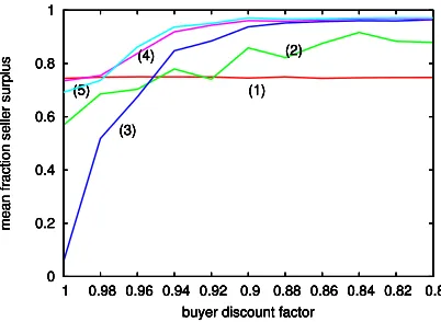
Figure 3 compares the obtained fraction of the totalseller surplusfor different seller threshold strategies and buyer dis-count factors (buyers have equal disdis-count factors). We de-fine the seller surplus of a bilateral negotiation as the seller’s maximum feasible utility, i.e., when the buyer offers her

0 0.2 0.4 0.6 0.8 1 0.8 0.82 0.84 0.86 0.88 0.9 0.92 0.94 0.96 0.98 1

mean fraction seller surplus

buyer discount factor (1) (2) (3) (4) (5) 0 0.2 0.4 0.6 0.8 1 0.8 0.82 0.84 0.86 0.88 0.9 0.92 0.94 0.96 0.98 1

buyer discount factor (1)

(2)

(3) (4)

[image:6.595.321.522.57.204.2]

(5)

Figure 3: Seller’s obtained fraction of total surplus for various discount factors and using 5 different threshold strategies: (1) fixed threshold, (2) time-dependent threshold, (3) responsive threshold, (4) combined (3) and (1), and (5) combined (3) and (2). The discount factor is set equal for all buyers.

imum threshold value and the offer is Pareto-efficient. As shown in Fig. 3, the fixed threshold strategy (1) is able to extract around 75% of the seller surplus. Note that the outcomes are independent of the discount factor when this strategy is used. Clearly, the fixed threshold strategy is un-able to benefit from the buyers’ time pressure.

The time-based threshold strategy (2), on the other hand, shows that higher profits can be obtained if the threshold changes in time, see Fig. 3. Buyers with a high valuation will purchase relatively early, since waiting for a better deal does not compensate the loss due to time discounting. Buyers with a low valuation, on the other hand, have the incentive to reach an agreement in a later stage if they can get a better price for it. This way the seller can indirectly discriminate between buyers with different valuations and time pressures.

Note that with no time discounting (i.e., when δ = 1) the fixed threshold strategy performs better. This is due to the difference in strategy complexity: only a single value needs to be optimized in case of a fixed threshold, whereas an en-tire function (encoded by 4 values) needs to be learned in case of the time-based threshold. This is clearly more diffi-cult, especially within a dynamic environment with learning buyers.

(7)

Strategy δ1 δ2 δ3 fraction seller surplus

[image:7.595.54.278.52.169.2]

1 1.0 0.95 0.90 0.75±0.09 2 1.0 0.95 0.90 0.76±0.12 3 1.0 0.95 0.90 0.55±0.08 4 1.0 0.95 0.90 0.86±0.09 5 1.0 0.95 0.90 0.84±0.08 1 0.95 0.90 0.85 0.75±0.09 2 0.95 0.90 0.85 0.85±0.08 3 0.95 0.90 0.85 0.86±0.07 4 0.95 0.90 0.85 0.95±0.04 5 0.95 0.90 0.85 0.95±0.04

Table 1: Mean fraction of seller surplus when the 3 buyer types have different discount factors. The strategies correspond to the seller threshold strate-gies in Fig. 3.

0 0.01 0.02 0.03 0.04 0.05 0.8 0.82 0.84 0.86 0.88 0.9 0.92 0.94 0.96 0.98 1 average inefficiency

(2)

(3) (4) (5) 0 0.01 0.02 0.03 0.04 0.05 0.8 0.82 0.84 0.86 0.88 0.9 0.92 0.94 0.96 0.98 1 average inefficiency

(2)

(3) (4) (5)

Figure 4: Average inefficiency of the agreements us-ing different strategies. The numbers correspond to the seller threshold strategies in Fig. 3.

in Fig. 3, this results in very good outcomes, even if buyers are very patient. This makes the combined strategy very versatile.

The above outcomes are based on experiments where buyers have equal time pressure. The results shown in Table 1, how-ever, indicate a similar outcome if different buyer types have different time preferences. Table 1 shows the mean fraction of surplus obtained by the seller given a discount factorδi

for buyers of typei, using the different threshold strategies. These outcomes in Table 1 also show that the responsive threshold strategy (no. 3) performs relatively poorly even if only one of the buyer types has no time pressure (in this case whenδ1= 1.0). This occurs since very little profits are

obtained from these buyers. As before, however, low profits can be prevented by adding a reservation value.

The mean (in)efficiency of the obtained bargaining results is depicted in Fig. 4. The inefficiency is measured as the seller’s maximum Pareto-improvement of a given outcome divided by the seller’s actual utility plus the improvement. The out-comes show low inefficiencies for all strategies (the highest inefficiency is around 2.7% of the total utility). However, relatively the responsive threshold strategies result in the most Pareto-efficient deals. Unlike the other strategies, the

responsive strategies set the threshold exactly to the best offer. Since this is the buyer’s best offer, it is already quite efficient. In case of the other strategies, however, the util-ity of the offers usually exceed the seller’s threshold, and the seller first needs to map the buyer’s offers to the right utility level when making counter offers. This mapping results in additional inefficiencies of the outcomes. Even with a rea-sonably simple strategy for determining the relative magni-tude of the attribute values, already good results are found. The Pareto-efficiency is expected to improve even further by incorporating more advanced strategies as described in e.g. [5, 9, 4, 10, 13]. This is however left for future work.

4.3 Bargaining Revisited

A possible strategy of the buyer agent is to bid very low, and then accept the counter offer of the seller. Such a strategy could be beneficial in case the seller’s counter offer is influ-enced by the buyers’ offers, as with the responsive thresh-old strategies. This could then result in low profits for the seller. To see if indeed buyers benefit from such a strategy, the strategy representation for buyers was extended by us-ing two separate functions: one produces the threshold for determining the utility level of the offers and the other func-tion determines the threshold for accepting or rejecting the seller’s offers (see Section 3.2). Even with separated func-tion, however, the responsive threshold strategy performs very much in favor of the seller (as shown by the results). This occurs because the counter offer is delayed by the seller whenever offers fall below the (seller’s) threshold, hence pro-viding the buyers with an incentive to try and get an agree-ment without delay.

5. CONCLUDING REMARKS

In this paper, we consider strategies for a seller agent who negotiates with many buyers simultaneously in a bilat-eral fashion over multiple interdependent attributes. These strategies respect a notion of fairness such that buyers are treated similarly. An important aspect of the developed strategies is their ability to benefit from impatient buyers that prefer early agreements. Buyers can have different val-uations and time preferences. A buyer’s actual valuation and time preference is only known to himself (i.e., a buyer’s type constitutes private information).

The strategies introduced determine three aspects: a thresh-old, multi-attribute offers with a utility level corresponding to the threshold, and a scheme for determining when to re-spond. Five different threshold strategies for the seller agent are evaluated and compared: (1) fixed threshold, (2) time-dependent threshold strategies, (3) responsive, (4) respon-sive with fixed reservation value, and (5) responrespon-sive with time-dependent reservation value. The last two strategies are actually a combination of the responsive threshold strat-egy with the first two strategies.

[image:7.595.68.276.238.386.2]

(8)

ex-clusively on the offers received by the buyers, and does not require any learning.

The outcomes show that bilaterally exchanging multiple of-fers combined with a random offer generation mechanism suffices for closely approximating Pareto-efficiency. Further-more, the responsive threshold strategies appear to be very successful in utilizing time pressure and consequently ex-tract a very high share of the surplus. For sufficiently high time pressure, the seller obtains almost all surplus, indicat-ing that buyers submit and/or accept offers close to their reservation value. Thus buyers self-select to pay their val-uation, while the bargaining outcomes respect our notion of fairness. The results also show superior performance of the combined strategies (4 and 5) compared to the auction-inspired strategy (3), in case some or all buyers have very little time pressure. In other words, the combined strategy is very versatile.

6. REFERENCES

[1] L. Ausubel and P. Cramton. Vickrey auctions with reserve pricing.Economic Theory, 23(3):493–506, 2004.

[2] T. B¨ack.Evolutionary Algorithms in Theory and Practice. Oxford University Press, New York and Oxford, 1996.

[3] D. Cliff. Explorations in evolutionary design of online auction market mechanisms.Electronic Commerce Research and Applications, 2:162–175, 2003. [4] H. Ehtamo and R. P. Hämäläinen. Interactive

multiple-criteria methods for reaching pareto optimal agreements in negotiations.Group Decision and Negotiation, 10:475–491, 2001.

[5] P. Faratin, C. Sierra, and N. R. Jennings. Using similarity criteria to make issue trade-offs.Journal of Artificial Intelligence, 142(2):205–237, 2003.

[6] S. Fatima, M. Wooldridge, and N. R. Jennings. Comparing equilibria for game theoretic and evolutionary bargaining models. InProc. 5th Int. Workshop on Agent-Mediated E-Commerce, Melbourne, Australia, pages 70–77, 2003. [7] E. Gerding, D. van Bragt, and J. La Poutr´e.

Multi-issue negotiation processes by evolutionary simulation: Validation and social extensions.

Computational Economics, 22:39–63, 2003.

[8] A. V. Goldberg and J. D. Hartline. Envy-free auctions for digital goods. InProceedings of the 4th conference on Electronic commerce, pages 29–35. ACM, ACM, 2003.

[9] M. Klein, P. Faratin, H. Sayama, and Y. Bar-Yam. Negotiating complex contracts.Group Decision and Negotiation, 12:111–125, 2003.

[10] R. J. Lin and S. cho T. Chou. Overcoming the fixed-pie bias in multi-issue negotiations. In

Proceedings Second International Conference in Electronic Business, 2002.

[11] S. Phelps, P. McBurney, S. Parsons, and E. Sklar. Co-evolutionary auction mechanism design: A preliminary report. In J. Padget, O. Shehory, D. Parkes, N. Sadeh, and W. Walsh, editors,

Agent-Mediated Electronic Commerce IV: Designing Mechanisms and Systems, volume 2531 ofLecture Notes in Computer Science, pages 123–142. Springer-Verlag, Berlin, 2002.

[12] A. Rubinstein. Perfect equilibrium in a bargaining model.Econometrica, 50(1):97–109, January 1982. [13] D. Somefun, E. Gerding, S. Bohte, and J. La Poutr´e.

Automated negotiation and bundling of information goods. In J. A. Rodriguez-Aguilar, P. Faratin, W. E. Walsh, and D. Parkes, editors,Workshop on Agent Mediated Electronic Commerce V: Designing Mechanisms and Systems, volume 3048 ofLecture Notes in AI, Heidelberg, 2004. Springer-Verlag. [14] L. Tesfatsion. (Guest Editor), Special issue on

Automated Bilateral Bargaining about Multiple Attributes in a One to Many Setting