C
ONDITIONALO
RDERINGU
SINGN
ONPARAMETRICE
XPECTILESY
VESA
RAGON,
S
ANDRINEC
ASANOVA,
R
AYC
HAMBERS ANDE
VEL
ECONTEA
BSTRACTC
ONDITIONAL ORDERING USING NONPARAMETRIC EXPECTILESYves Aragon*, Sandrine Casanova*, Ray Chambers†& Eve Leconte*
* G.R.E.M.A.Q., Universit´e des Sciences Sociales, 21, all´ee de Brienne, 31000 TOULOUSE, France
and
L.S.P., Universit´e Paul Sabatier,
118, route de Narbonne, 31062 TOULOUSE Cedex 4, France
†Southampton Statistical Sciences Research Institute
University of Southampton, Highfield, Southampton SO17 1BJ, United Kingdom
E-mail : [email protected], [email protected], [email protected], [email protected]
Abstract. Expectile regression, and more generally M-quantile regression, can be used to characterise the relationship between a response variable and explanatory variables when the behaviour of ”non-average” individuals is of interest. The aim of this paper is to demonstrate how an individual’s expectile-order, based on nonparametric estimation of the expectile regression function, can also be used to define a conditional ordering of the individual’s value relative to the values of other members of a data set. The relationship between contextual, or ”grouping”, variables and this ordering can then be investigated. In particular, we propose five estimators of expectile-order, which we compare via simula-tion. The use of estimated expectile-order to investigate grouping effects is then illustrated using data on physician prescribing behaviour in the Midi-Pyr´en´ees region of France dur-ing 1999.
Keywords: conditional expectile, expectile regression, asymmetric regression, local
re-gression, monotonization techniques, order estimation, ordering index
1
Introduction
the Midi-Pyr´en´ees region of France in 1999. This ordering is with respect to their drug prescribing behaviour and conditions on the characteristics of their practice and other relevant variables. A major problem with constructing such an order-ing is that of heteroskedasticity in the regression relationship. In particular, the values associated with individuals whose behaviour deviates from the mean may just reflect heteroskedasticity induced by explanatory variables rather than any intrinsic characteristics of these individuals. Such heteroskedasticity is usually accounted for by a weighted regression fit. However, such an approach typically requires some form of parametric specification for both the regression function and the associated heteroskedasticity, and often assumes errors are symmetrically distributed. There are nonparametric approaches to fitting heteroscedastic models (see Welsh, 1996), but these can be complex. In contrast, we tackle the problem directly by modelling the conditional quantiles of the response given the explana-tors. Quantiles are part of a general class of distributional location functionals that Breckling and Chambers (1988) refer to as M-quantiles. Beside quantiles, this class contains the expectiles, which generalize the expectation in the same way as quantiles generalize the median (Newey and Powell, 1987), and we base our ordering method on application of this method.
In order to motivate our approach, we consider the problem of monitoring drug prescribing behaviour mentioned above. In particular, letY be the average value of prescriptions issued by a physician over some fixed period, and assume that a regulatory body (e.g. the Social Security Administration or SSA) has an interest in ranking all physicians in a certain region according to their values ofY. This may be because the SSA wants to identify individual physicians whose prescribing be-haviour is substantially different from average prescribing bebe-haviour, or it may be because the SSA is interested in identifying whether there are ”groupings” in these ranks associated with particular regions, indicating inequalities in sub-regional prescription expenditure. In either case, suppose that one assumes that a physician with average prescription value above some threshold, sayy0, generates
a ”loss” for the SSA. Then the average loss per physician is:
IE((Y −y0)I(Y > y0)) (1)
while the probability of a physician exceeding this threshold is
IE(I(Y > y0)). (2)
In practice y0 is unknown, but we can use the above framework to motivate
an approach to ranking individual physicians on the basis of their potential finan-cial risk to the SSD prescription budget. In particular, consider a physician with
Y =yi and X=xi. Here X denotes the (vector-valued) random variable
charac-terising the distribution of physician characteristics across the region of interest. The expected additional loss to the SSD prescription budget caused by an increase in the average value of prescriptions issued by this physician is then
IE((Y −yi)I(Y > yi)|X=xi). (3)
A dimension free version of this expected additional loss is obtained by dividing (3) by the average absolute departure fromyi, i.e. IE(|Y −yi| |X=xi), leading
to the normalized coefficient
IE(|Y −yi|I(Y > yi)|X=xi)
IE(|Y −yi| |X=xi)
· (4)
In particular, the higher the value of this ratio, the lower the financial risk asso-ciated with the physician, since the expected loss due to him or her increasing prescription expenditure relative to its current level is greater. In other words, the physician is relatively cheap (in terms of prescription expenditure and after accounting for personal and practice characteristics) as far as the current SSA prescription budget is concerned (Newey and Powell, 1987). Consequently, in or-der to associate a high ranking with a high risk, we work with the complementary ratio
qi =
IE(|Y −yi|I(Y ≤yi)|X=xi)
IE(|Y −yi| |X=xi)
(5)
which we refer to as the expectile-order of the physician’s prescribing behaviour. The higher the valueqi, the more risky the physician is for the SSA prescription
budget. Notice also that (5) parallels the quantile-order of the physician’s average prescription expenditure, defined by
IE(I(Y ≤yi)|X=xi)
IE(1|X=xi)
(6)
which corresponds to the probability that a physician with characteristic xihas an
average prescription expenditure less than or equal to yi. Since the level of
ex-penditure is of greater interest here than its associated rank, we argue that ranking based on expectile-order is more suitable than ranking based on quantile-order in this situation.
now generalise the concept of expectile-order so that it applies to arbitrary values ofY and X. In order to do so, we provide a more rigorous definition of expectile regression. LetF(.|X=x)denote the cumulative distribution function (c.d.f.) of
Y given X=x. Consider the minimization problem
min θ
Z
ρq(y−θ)dF(y|X=x) (7)
whereρqis a loss function andqis fixed,0< q <1. Differentiating the objective
function in (7) with respect toθ leads to the estimating equation Z
ψq(y−θ)dF(y|X=x) = 0 (8)
whereψq(u) = δρq(u)/δuis called the influence function. It is well known that if
ψq(.)equalsqfor positive values of its argument and equals−(1−q)for negative
values of its argument, then the solution to (7) and (8) is the q-quantile of the conditional distributionF(.|X=x). In contrast, theq-expectile of this conditional distribution is defined by setting
ψq(u) =
(
qu if u≥0
(1−q)u if u <0 (9)
in (8). Note that this corresponds to the asymmetric least squares loss function
ρq(u) =
(
qu2
if u≥0 (1−q)u2
if u <0. (10)
The conditional q-expectile is unique (see Newey and Powell, 1987) and is de-notedm(q,x)in what follows. Furthermore, the 0.5-expectile is the expectation of the conditional distribution F(.|X = x). Substituting the influence function defined by (9) into (8), one obtains a formal definition of m(q,x)as the solution of the equation
q= IE(|Y −m(q,x)|I(Y ≤m(q,x))|X=x)
IE(|Y −m(q,x)| |X=x) · (11)
The general definition of the expectile-order of a sample unit with values(yi,xi)
is then the valueqi that satisfies the identitym(qi,xi) =yi.
extend the concepts of quantile and expectile regression toM-quantile regression and also define a multivariate M-quantile. Yao and Tong (1996) propose a non-parametric estimator of conditional expectiles based on local linear polynomials with a one-dimensional covariate, and establish the asymptotic normality and the uniform consistency of their estimator.
In this paper we focus on the application of expectile-order to the problem of ordering economic performance data, as in Kokic et al. (1997). As noted earlier, standard residuals are inadequate in this case because they are sensitive to con-ditional heteroscedasticity in the data. Instead, we use a nonparametric expectile regression model to estimate the expectile-order. In section 2, we propose five estimators of the expectile-order. The first four require nonparametric estimation of conditional expectiles as a first step, whereas the last one is obtained directly. We compare these estimators using simulated data in section 3. Finally, in section 4, we apply our methods to defining an ordering of a data set containing informa-tion about the characteristics and average prescripinforma-tion values of physicians in the Midi-Pyr´en´ees region of France in 1999.
2
Estimation of expectile-orders
In this section we propose five estimators of the expectile-order for the case where the response variableY is univariate, and the covariate X is a vector in IRp. Four of the procedures estimate the expectilesm(q,x)on a grid ofq values and then, for any given observation, use linear interpolation or logistic smoothing to obtain the corresponding q. The methods are distinguished by the fact that they esti-mate m(q,x)by a locally constant Nadaraya-Watson kernel estimator, a locally linear kernel estimator, a locally linear mean preserving monotone kernel estima-tor and a locally linear isotonic regression kernel estimaestima-tor. The fifth estimates the expectile-order directly. The observed sample values are denoted (Yi,Xi)ni=1
in what follows.
2.1
Expectile-order based on locally constant expectile
regres-sion
A kernel-based estimatormLC(q,x)ofm(q,x)that is equivalent to fitting a local
constant to this function is the solution to the minimization problem
min θ∈R
Z
where
ˆ
Fn(y|X=x) = n
X
i=1
K(x−Xi
h )I(Yi ≤y)
n
X
i=1
K(x−Xi
h )
is the Nadaraya-Watson kernel estimator of the conditional c.d.f. F(.|X= x), K
is a multivariate kernel function, h is a vector of suitable bandwidths and the loss functionρq is defined by (10). Differentiating (12) with respect toθ leads to the
estimating equation
n
X
i=1
ψq(Yi−θ)K(
x−Xi
h ) = 0 (13)
withψqas in (9). DefiningVq,i(x) = (Ii−2qIi+q)K(
x−Xi
h )whereIi =I(Yi ≤
θ) and solving (13) leads to the estimatormLC(q,x), which can be written as a
weighted average of the sample values ofY,
mLC(q,x) = n
X
i=1
Vq,i(x)Yi
n
X
i=1
Vq,i(x)
· (14)
For general q the estimatormLC(q,x)can only to be computed iteratively since
Vq,i(x)depends onθ. This estimator is strictly monotone increasing inq, so that
an estimator qLC(y,x) of the expectile-order of an observation with Y = y can
be directly computed by linear interpolation over a grid of values ofqdefined for each value of x. That is, ifqLandqU are the two adjacent values on this grid such
thatmLC(qL,x)< y < mLC(qU,x)then the estimated expectile-order of a sample
unit with valuesyand x isq(y,x) =α(y,x)qL+ (1−α(y,x))qU where
α(y,x) = mLC(qU,x)−y
mLC(qU,x)−mLC(qL,x)
· (15)
2.2
Expectile-orders based on local linear estimators
Alternatively we consider nonparametric estimation of the expectile regression function based on a kernel weighted local linear fit (Yao and Tong, 1996). Given ap×1vector u we define u∗0 = [1u0]. A locally linear nonparametric estimator ofm(q,x)is then
mLL(q,x) =x∗
0ˆ
whereβˆq(x)is the solution to the minimization problem
min
b∈Rp+1 Z
ρq(y−x∗
0
b)dFˆn(y|x). (17)
Differentiating (17) with respect to b leads to the estimating equation
n
X
i=1
ψq(Yi−X∗
0
i b)K(
x−Xi
h )X
∗0
i = 0. (18)
Let Y be the n × 1 vector of sample data for the response variable, X∗0
= [X∗10· · ·X∗
0
n] with X∗
0
i defined similarly as u∗
0
and letVq(x) be the n×n
diago-nal matrix of weights {Vq,i(x)}, where the Vq,i(x) were defined in the previous
section. The solution to (18) is then
ˆ
βq(x) = (X∗
0
Vq(x)X∗)−
1
X∗0Vq(x)Y.
Note thatβˆq(x)must also be computed iteratively since the matrixVq(x)depends
on b.
The estimator mLL(q,x) is not necessarily a nondecreasing function of q at
every value of x. That is, the fitted expectile surfaces obtained by solving (18) can cross in the sample x-data range. This problem is also discussed in Kokic et
al. (1997). He (1997) describes a restricted version of quantile regression that
avoids such crossing. Craig and Ng (2001) encounter the same problem when using smoothing splines to estimate conditional quantiles in an analysis aimed at identifying employment subcenters in a multicentric urban area. Here we tackle this problem by constraining the estimatormLL(q,x)so that it is monotone with
respect to the values q on a grid Q defined at every sample value of x. In par-ticular we adapt the technique of Mukarjee and Stern (1994) so that, for qin Q, the estimatormLL(q,x)is replaced by the mean preserving monotone estimator
mM P M(q,x)
mM P M(q,x) =
(
minq0∈Q, q≤q0≤0.5mLL(q0,x) if q∈]0,0.5]
maxq0∈Q,0.5≤q0≤qmLL(q0,x) if q∈]0.5,1[
An alternative approach is to use isotonic regression (Robertson et al., 1998) to construct a monotone estimator ofm(q, x). This leads to the estimatormIRM(q,x),
which is the nearest monotone estimator ofm(q, x)according to the L2norm. Let
Q ={q1,· · ·, qs}be the grid of values ofqwithq1 ≤ · · · ≤qs. Then forqi inQ,
mIRM(qi, x)is defined by
mIRM(qi,x) = min
whereAv(X1,· · ·, Xm)is the empirical mean of the sequenceX1,· · ·, Xm. For
both methods of monotonization, the estimated expectile-order of each observa-tion (y,x) is then calculated by linear interpolation as in (15), leading to two estimators ofqthat we denote byqM P M(y,x)andqIRM(y,x)respectively.
Finally, as an alternative to direct monotonization of the conditional expec-tiles, one can fit a linear model to the logits of the values in the gridQusing the estimated conditional expectile valuesmLL(q,x)calculated on this grid at a fixed
value x as explanators. The estimated expectile-orderqLR(y,x)for a point(y,x)
is then obtained as the predicted value generated by this model at the valuey.
2.3
A direct estimator of the expectile-order
From (11) we see that the value y of a data point (y,x)is the expectile m(q,x)
where
q= IE(|Y −y|I(Y ≤y)|X=x)
IE(|Y −y||X=x) · (19)
For each (y,x), we can estimate the numerator and the denominator of (19) us-ing weighted Nadaraya-Watson type kernel estimators (Hall et al., 1999). The resulting estimator of the expectile-order is then
qALN W(y,x) = n
X
i=1
|Yi−y|I(Yi ≤y)K(
x−Xi
h )wi(x)
n
X
i=1
|Yi−y|K(
x−Xi
h )wi(x)
, (20)
where the wi(x)’s define a set of calibrating weights, i.e. they satisfy wi ≥ 0,
X
i
wi = 1and
X
i
(Xi−x)K(
Xi−x
h )wi(x) = 0.
The above constraints do not uniquely define the wi(x)’s, and so we calculate
these weights by minimisingX
i
w2
i subject to these constraints. This ensures that
wi stays close to 1
n. Put ui(x) = (Xi −x)K(
Xi−x
h ). Thep×nmatrixU(x)is
then defined byU(x) = (u1(x)u2(x) · · ·un(x))withU¯(x)∈IRp the mean vector
of the rows ofU. Straightforward calculation yields
(w1(x)w2(x)· · ·wn(x))0 =
1
n1n−
|A(x)|
|B(x)|(U(x)−
¯
whereA(x) =U(x)U0(x)andB(x) = (U(x)−U¯(x)10
n)(U(x)−U¯(x)10n)0arep×p
matrices. Note that Hall et al. (1999) define the weightswiso that they maximize
Q
iwi, i.e. these authors seek to minimise the Kullback distance of{wi}from 1
n.
Unfortunately, we experienced convergence problems when attempting to apply this criterion. Furthermore,qALN W(y,x)is a nondecreasing function ofybecause
(20) is equal to (19) when the conditional distribution functionF(y|X=x)is
n
X
i=1
K(x−Xi)
h )wi(x)I(Yi ≤y)
n
X
i=1
K(x−Xi
h )wi(x) ·
Using the results in Hall et al (1999), it can be shown that the numerator and
the denominator of qALN W (both divided by n
X
i=1
K(x−Xi
h )wi(x)) are local
lin-ear estimators in which the weights are K(x−Xi
h )wi(x) instead ofK( x−Xi
h ).
Furthermore, under suitable regularity conditions, these estimators are first order equivalent to classical local linear estimators. Finally, we observe that since the computation of (20) is very fast, an estimatormALN W(q,x)ofm(q,x)can be
de-rived as follows. We first calculate the estimated expectile-ordersqALN W(y,x)on
a very fine grid of y values. Then, for a given value q and a fixed value of the covariate x,mALN W(q,x)is obtained by linear interpolation.
3
A simulation study
3.1
Description
In this section we investigate the finite sample performance of the five estimators of the expectile regression functions that were defined in the previous section, as well as their corresponding estimators of the expectile-orders of the sample values. Data values forS = 500samples, each of sizen = 200were simulated, with the covariate X defined as the sum of two independent variables uniformly distributed on [0,2.5]and the value of Y given X = x drawn from a Gaussian distribution with mean m(x) = 20 + (0.8x− 2)3
and standard deviation 2.5. With this definition, the corresponding conditional q-expectile of Y at X = x
is m(q, x) = m(x) + 2.5eq, whereeq is theq-expectile of a standard Gaussian
three separate cross validation exercises. Since the choice of bandwidth precedes monotonization, the estimators mM P M and mIRM used the same bandwidth as
mLL. Bandwidth choice for the estimatorsmLC andmLLwas based on extending
the classical least squares cross-validation technique to the case of expectiles, with the selected bandwidth minimizing
n
X
i=1
ρq(Yi−mEST,−i(q, Xi))
on a grid of 20 regularly spaced bandwidth values in [0.8,5] (the length of this interval roughly corresponds to the range of the covariate). Here ESTdenotes the type of smoother used (LC orLL) andmEST,−i is calculated using the data set
{(yj, xj), j 6=i}.
A cross-validation criterion was also used to determine the bandwidth for the direct estimator of expectile-order. For a given observation(yi, xi),we define the
random variables
Y1i =|Y −yi|I(Y ≤yi) and Y2i =|Y −yi|.
Let (Y1ij, Xj)nj=1 and (Y2ij, Xj)nj=1 be the observed sample data. Letm1i(x) =
IE(Y1i|X = x) and m2i(x) = IE(Y2i|X = x). The true expectile-order of the
observation (yi, xi) is then q(yi, xi) =
m1i(xi)
m2i(xi)
and the estimatorqAN LW(yi, xi)
is mˆ1i(xi)
ˆ
m2i(xi)
wheremˆki(xi), k = 1,2, is the weighted Nadaraya-Watson estimator
of the conditional mean mki(xi). Optimal bandwidths for themˆki(xi), k = 1,2,
i= 1,· · ·, nare then obtained by minimizing
n
X
i=1
n
X
j=1
(Ykij−mˆki,−j(xi))
2
, k = 1,2 (21)
where cmki,−j, k = 1,2, is calculated using the data set {(yl, xl), l 6= j}. A
Taylor expansion of qALN W in the neighborhood of (m1i(xi), m2i(xi)) leads to
the approximation
qALN W(yi, xi)'
m1i(xi)
m2i(xi)
+ai( ˆm1i(xi) +bimˆ2i(xi))
withai = 1
m2i(xi)
andbi =−
m1i(xi)
m2i(xi)
. The same bandwidth is then used in both
numerator and denominator ofqALN W, and is chosen so that n
X
i=1
n
X
j=1
is minimized. The coefficients bi in this expression are estimated using the
com-ponent specific optimal bandwidths determined by minimizing (21).
The estimatorsmLC(q, x),mLL(q, x),mM P M(q, x),mIRM(q, x)andmALN W(q, x)
of the conditional expectile function were then computed for a set ofM = 49 reg-ularly spaced values{x1,· · ·, xM}ofxin[0.1,4.9]and for a grid ofL= 9values
ofq, corresponding toQ={.01, .05, .1, .2, .5, .8, .9, .95, .99}. Since we know the true conditional expectile function, the mean squared error (MSE) of each estima-tormEST(q, x)ofm(q, x)can be evaluated as
MSE(mEST, q, x) = 1
S
S
X
s=1
(mESTs(q, x)−m(q, x))
2
,
wheremESTs denotes the estimator ofmfor thesth sample. We also compute the
mean averaged squared error (MASE) defined by
MASE(mEST, q) = 1
SM
S
X
s=1
M
X
m=1
(mESTs(q, xm)−m(q, xm))
2
.
For EST in the set {LC, MP M, IRM, LR, ALNW}, the performance of an estimator qEST(y, x)of the expectile-order of a data value (y, x), based on
cor-responding estimated conditional expectile functions at each value q in the grid
Q, is then evaluated by calculating its mean absolute deviation error (MADE) for each samples(see Hall et al., 1999),
MADE(qESTs) =
1
LM
L
X
l=1
M
X
m=1
|qESTs(ylm, xm)−ql|, s= 1,· · ·, S,
whereylm satisfiesm(ql, xm) = ylm.
3.2
Results
3.2.1 Estimators of conditional expectile functions
Table 1 shows the values of MASE for q in Q. Notice that the estimator mLL
performs better than the estimator mLC and that monotonization leads to an
im-provement in MASE. The monotonized estimatorsmM P MandmIRMhave similar
performances, with mM P M performing better for extreme values ofqandmIRM
performing better for values of q close toq = 0.5. The estimatormALN W
q mLL mM P M mIRM mLC mALN W
[image:13.595.176.436.121.266.2].01 1.8239 1.7425 1.7781 2.6970 0.8712 .05 1.2641 1.1527 1.1787 1.9860 0.9757 .1 .84825 .82594 .82987 1.3145 0.9313 .2 .71979 .71043 .69274 1.1940 0.8718 .5 .61578 .61578 .59281 1.1305 0.8718 .8 .71693 .71042 .69471 1.1924 0.8917 .9 .88439 .85448 .84264 1.3061 0.9562 .95 1.2637 1.1829 1.1906 2.0011 1.0164 .99 1.8681 1.8054 1.8239 2.7129 0.9126
Table 1: Values of MASE for estimators of conditional expectiles at the values of
qinQ.
0.02 0.04 0.06 0.08 0.1 0.12
MADE
MPM IRM LR LC ALNW
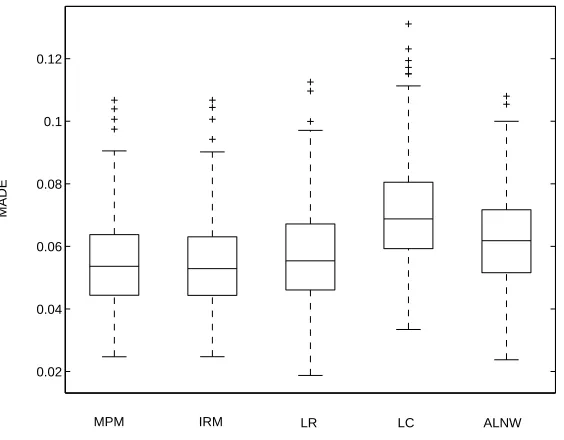
[image:13.595.167.449.369.589.2]3.2.2 Estimators of expectile-orders
Boxplots of MADE for the five estimators qM P M, qIRM, qLC, qLR and qALN W
of expectile-orders are shown in Figure 1. As with estimation of conditional ex-pectiles, the estimatorsqM P M andqIRM based on local linear regression perform
better than the estimatorqLCbased on locally constant regression and the direct
es-timatorqALN W. The median MADE value for the estimatorqLRis only marginally
higher than the median MADE values ofqM P M andqIRM. However, its variability
is greater. On the basis of these rather limited simulation results, it appears that the expectile-order estimators qM P M and qIRM based on monotonized expectile
fits may be preferable.
4
An application
4.1
The data set
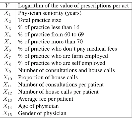
We focus on a data set that contains measurements on 2801 physicians in the Midi-Pyr´en´ees region of France during 1999, including most of the general prac-tice physicians in this region. The study variable, denotedY, measures the drug prescribing activity of a physician, and is defined as the logarithm of the ratio of the value of drug prescriptions issued by the physician over the year divided by the number of ”acts” carried out by the physician over the same period. An act may be a house call or a consultation. In addition to this variable, the data set contains a number of indicators of a physician’s practice and activity characteristics as well as the physician’s age and gender. These variables are denoted X1,· · ·, X15and
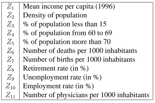
are listed in Table 2. Each physician works in a canton (a small county). For each canton we also have demographic statistics and other characteristics, e.g. level of education and level of unemployment. These variables are denoted Z1,· · ·, Z11
Y Logarithm of the value of prescriptions per act
X1 Physician seniority (years)
X2 Total practice size
X3 % of practice less than 16
X4 % of practice from 60 to 69
X5 % of practice more than 70
X6 % of practice who don’t pay medical fees
X7 % of practice who are farm employed
X8 % of practice who are self employed
X9 Number of consultations and house calls
X10 Proportion of house calls
X11 Number of consultations per patient
X12 Number of house calls per patient
X13 Average fee per patient
X14 Age of physician
[image:15.595.173.438.96.334.2]X15 Gender of physician
Table 2: Physician and practice variables.
4.2
Dimension reduction
Nonparametric regression can become unstable if there are many covariates. Since the ordering methodology described in this paper depends on a predictive, rather than interpretative, regression model, it is advisable to reduce the dimension of the covariate space by taking into account the dependence between the covariates and the response variable. This can be done through a Sliced Inverse Regression (SIR) analysis (Li, 1991, and Cook, 1994, 1996). This method is a fast exploratory analysis tool producing a small number of synthetic indices (linear combinations of the covariates). Nonparametric regression modelling then proceeds using these indices as covariates. A SIR of the response variable based on the physician and practice variables in table 2 gives 6 major eigenvalues (see Table 4).
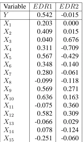
These eigenvalues fall sharply after the second eigenvalue. Consequently we use the first two SIR indices as covariates in the nonparametric regression fit to the expectiles of the value of drug prescription per act. These indices are denoted
EDR1andEDR2in what follows. Table 5 shows the correlations between these two indices and the variablesY, X1,· · ·, X15used in the SIR. The dependent
vari-able appears first.
asso-Z1 Mean income per capita (1996)
Z2 Density of population
Z3 % of population less than 15
Z4 % of population from 60 to 69
Z5 % of population more than 70
Z6 Number of deaths per 1000 inhabitants
Z7 Number of births per 1000 inhabitants
Z8 Retirement rate (in %)
Z9 Unemployment rate (in %)
Z10 Employment rate (in %)
[image:16.595.179.432.97.265.2]Z11 Number of physicians per 1000 inhabitants
Table 3: Canton variables.
0.3206 0.1841 0.0330 0.0203 0.0134 0.0107
Table 4: Eigenvalues of SIR
ciated with the level of activity of the physician, the percentage of old persons in the practice and the average fee per patient. In contrast EDR2is highly associ-ated with the percentage of young people in the practice and the percentage of the practice aged from 60 to 69.
In an effort to improve the estimation of these expectiles and of the conse-quent expectile-orders, we also investigated bringing the canton variables in Table 3 into the regression model. Here we performed a SIR of the amount of drug prescription per act on the combined set of variables X1,· · ·, X15, Z1· · ·, Z11,
with values of the variables Z1,· · ·, Z11 replicated for each physician in a
can-ton. From an inspection of the resulting eigenvalues we again decided to retain two indices. Both were highly correlated with the corresponding indices identi-fied from the first SIR (correlations of .984 and .959 respectively). Consequently, the introduction of canton level effects did not lead to any real change in the SIR indices, and so we proceeded to estimate the expectile-orders of the physicians in our data set conditioning only on the SIR indicesEDR1andEDR2based onY
Variable EDR1 EDR2
Y 0.542 -0.015
X1 0.203 0.000
X2 0.409 0.015
X3 0.040 0.676
X4 0.311 -0.709
X5 0.567 -0.429
X6 0.348 -0.140
X7 0.280 -0.061
X8 -0.099 -0.118
X9 0.569 0.271
X10 0.636 0.163
X11 -0.075 0.360
X12 0.582 0.309
X13 -0.066 0.029
X14 0.078 -0.124
[image:17.595.233.379.96.346.2]X15 -0.251 -0.060
Table 5: Correlations between SIR indices and physician and practice variables.
4.3
Measuring the quality of an expectile fit
In standard linear regression, the adjusted coefficient of determination is used to measure the quality of the regression fit, with a low value of this coefficient indicating low explanatory power or the presence of misspecification. To avoid misspecification issues, we use local regression techniques to estimate conditional expectiles. Replacing the ‘square’ function by the loss functionρqdefined by (10),
we adapted the adjusted coefficient of determination to the case of local expectile regression, leading to the coefficient
R2
q = 1−
n
X
i=1
ρq(yi−mEST(q,xi))/(n−ν(q))
n
X
i=1
ρq(yi−mˆ(q))/(n−1)
·
Heremˆ(q)denotes the unconditional empiricalq-expectile ofY, that is the value
of θ that minimizes
n
X
i=1
ρq(yi −θ), and EST belongs to {LL, LC}. The local
mEST(q,x) = n
X
i=1
li(q,x)yi (see Loader, 1999). As in linear regression, the
con-stantν(q)is therefore defined as the trace of the matrixL(q) = [lj(q,xi)]j
=1,···,n
i=1,···,n.
By definitionR2
q is a global measure of the quality of the local expectile
re-gression of orderq. As with the usual coefficient of determination, a low value of
R2
q indicates low dependence ofY on X, so that the conditional distribution ofY
is not well described by X. In such a situation the resulting expectile-order esti-mates will not be reliable. Notice that R2
q can also be used as a model-selection
tool.
4.4
Expectile modelling of the physician and practice variables
We estimated the expectile-orders of the physicians using the estimatorqM P M
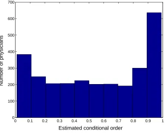
de-scribed in section 2, with an interpolation gridQ={.01, .1, .2, .5, .8, .9, .99}. As in the simulations, we used a locally linear smoother with a bivariate Epanech-nikov kernel with bandwidths set to 20%of the range of each SIR index. Figure 2 is the histogram of the resulting estimated expectile-orders. Physicians with es-timated expectile-orders in the tails of this distribution can be considered to have displayed extreme prescribing behaviour (in both a negative as well as a positive sense) relative to physicians with similar characteristics in the Midi-Pyr´en´ees re-gion in 1999. Note that the ”high cost” physicians are more numerous than the ”low cost” physicians. This can be contrasted with quantile orders, which are necessarily uniformly distributed.
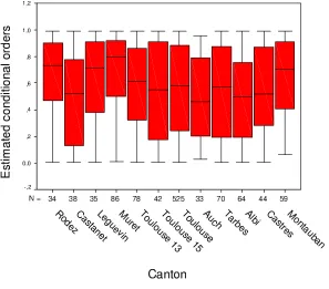
A question of some interest is the extent to which the variation in expectile-orders of individual physicians can be explained by canton-level effects. The pres-ence of such effects in these estimated expectile-orders can be seen in Figure 3. This shows the boxplots of estimated expectile-orders for the 12 larger cantons. Note that the median of these orders varies significantly between cantons. Thus, for the canton of Rodez, a rich rural canton, the median of these orders is close to 0.8 whereas for the canton of Auch, the median is just above 0.4. For the canton of Toulouse, the main city of the Midi-Pyr´en´ees region, the median is near 0.6. An analysis of variance of the logit of the expectile-orders with respect to the canton variable indicates that the average value of the estimated expectile-order varies significantly between cantons (p= 0.030).
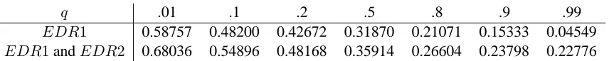
Finally, in Table 6 we show the values of theR2
q coefficient for different
val-ues ofq and two sets of explanatory variables: the first where the nonparametric regression fit is carried out using only the first SIR indexEDR1and the second one where this fit is based on bothEDR1andEDR2. Notice that takingEDR2
into account improves the fit at each value ofq. Notice also thatR2
decreas-0 0.1 0.2 0.3 0.4 0.5 0.6 0.7 0.8 0.9 1 0
100 200 300 400 500 600 700
Estimated conditional order
[image:19.595.140.475.234.506.2]Number of physicians
q .01 .1 .2 .5 .8 .9 .99
EDR1 0.58757 0.48200 0.42672 0.31870 0.21071 0.15333 0.04549
[image:21.595.114.542.99.142.2]EDR1andEDR2 0.68036 0.54896 0.48168 0.35914 0.26604 0.23798 0.22776
Table 6: Values of adjusted R2
q coefficient for one and two SIR indices and for
different values ofq.
ing function ofqin Table 6. Justification for this behaviour can be seen in Figure 4. This shows that, conditionally onEDR1, small values ofY (corresponding to small expectile-orders) are more sensitive to variation inEDR1than large values ofY.
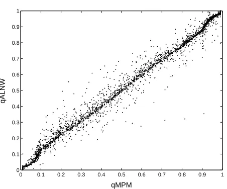
The conditional expectile-orders of physicians in the Midi-Pyr´en´ees region were also estimated directly usingqALN W. Computation of this estimator is
ex-tremely fast (typically 1000 times quicker than for the estimatorqM P M). A
scatter-plot of qALN W versusqM P M (see Figure 5) shows that these estimators coincide
for most physicians in the data set, with a correlation of 0.99. Note that direct estimation of the expectile-order is appropriate when comparison of sample in-dividuals is of primary interest. On the other hand, estimators of the expectiles curves may be useful when a global description of the conditional distribution is required.
5
Discussion
• • • • • • •• • • • • • • • • • • • • • • • • • • • • • • • • • • • • • • • • • • • • • • • • • • • • • • • • • • • • •• •• • • • • • • • • • • • • • •• • • • • • • • • • • • • • • • • • • • • • • • • • • • • • • • • • • • • • • • • • • • • • • • • • • • • • • • • • • • • • • • • • • • • • • • • • • • • • • • • • • • • • • • • • • • • • • • • • • • • • • • • • • • • • • • • • • • • • • • • • • • • • • • •• • • • • • • • • • • • • • • • • • • • • • • • • • • • • • • • • • • • • • • • • • • • • •• • • • • • • • • • •• • • • • • • • • • • • • • • • • • • • • • • • • • • • • • • • • • • • • • • • • • • • • • • • • • • • • • • • • • • • • • • • • • • • • • • • • • • • • • • • • • • • • • • • • • • • • • • • • • • • • • • • • • • • • • • • • • • • •• • • • • • • • • • • • • • • • • • • • • • • • • • • •• • • • • •• • • • • • • • • • • • • • • • • • • • • • • • • • • • • • • • • • • • • • • • • • • • • • • • • • • • • • • • • • • • • • • • • • • ••• • • • • • • • • • • • • • • • • • • • • • • • • • • • • • • • • • •• • • • • • • • • • • • • • • • • • • • • • • • • • • • • • • • • • • • • • • • • • • • • • • • • • • • • • • • • • • • • • • • • • • • • • • • • • • • • • • • • • • • • • • • • • • • • • • •• • • • • • • • • • • • • • • • • • • • • • • • • • • • • • • • • • • • • • • • • • • • • • • • • • • • • • • • • • • • • • • • • • • • • • • • • • • • • • • • • • • • • • • • • • • • • • • • • • • • • • • • • • • • • • • • • • • • • • • • • • • • • • • • • • • • • • • • • • • • • • • • • • • • • • • • • • • • • • •• • • • • • • • • • • • • • • • • • •• • • • • • • • • • • • • • • • • • • • • • • • • • • •• • • • • • • • • • • • • • • • • • • • • • • • • • • •• • • • • • • • • • • • • • • • • • • • • • • • • • •• • • • • • • • • • • • • • • • • • • • • • • • • • • • • • • • • • • • • • • • • • • • • • ••• • • • • • • • • • • • • • • • • • • • • • • • • • • • • • • • • • • • • • • • • • • • • • • • • • • • • • • • • • • •• • • • • • • • • • • • • • • • • • • • • • • • • • • • • • • • • • • • • • • • • • • • • • • • • •• • • • • • • • • • • • • • • • • • • • • • • • • • • • • • • • • • • • • • • • • • • • • • • • • • • • • • • • • • •• • • • • • • •• • • • • • • • • • • • • • • • • • • • • • • • • • • • • • • • • • • • • • • • • • • • • • • • • • • • • • • • • • • • • • • • • • • • • • • • • • • • • • • • • • • • • • • • • • • • • • • • • • • • • • • • • • • • • • • • • • • • • • • • • • • • • • • •• • • • • • • • • • • • • • • • • • • • •• • • • • • • • • • • • • •• • • • • • • •• • • • • • • • • • • • • • • • • • • • • • • • • • • • • • • • • •• • • • • • • • • • • • • • • • • • • • • • • • • • • • • • • • • • • • • • • • • • • • • • • • • • • • • • •• • • • • • • • • • • • • • • • • • • • • • • • • • • • • • • • • • • • • • • • • • • • • • • •• • • • • • • • • • • • • • • • • • • • • • • • • • • • • • • • • • • • • • • • • • • • • • • • • • • • • • • • •• • • • • • • • • • • • • • • • • • • • • • • • • • • • • • • • • • • •• • • • • • • •• • • • ••• • • • • • • • • • • • • • • • • • • • • • • • • • • • • • • • • • • • • • • • • • • • • • • • • • • • • • • • • • • • • • • • • • • • • • • • • • • • • • • • • • • • • • • • • • • •• • • • • • • • • • • • • • • • • • • • • • • • • • • • • • • • • • • • • • • • • • • • • • • • • • • • •• • • • • •• • • • • • • • • • • • • • • • • • • • • • • • • • • • • • • • • • • • • • • • • • • • • • • •• • • • • • • • • • • • • • • • • • • • • • • • • • • • • • • • • • • • • • • • • • • • • • • • • • • • • • • • • • • • • • • • • • • • • • • • • • • • • • • • • • • • • • • • • • • • • • • • • • • • • • • • • • • • • • • • • • • • • • • • •• • • • • • • • • • • • • • • • • • • • • • • • • • • • • • • • • • • • • • • • • • • • • • • • • • • • • • • • • • • • • • • • • • • • • • • • • • • • • • • • • • • • • • • • • • • • • • • • • • • • • • • • • • • • • • • • • • • • • • • • • • • • • • • • • • • •• • •• • • • • • • • • • • • • • • • • • • • • • • • • • • • • • • • • • • • • • • • • •• • • • • • • • • •• •• • • • • • • • • • • • • • • • • • • • • • • • • • • • • • • • • • • • • • • • • • • • • • • • • • • • • • • • • • • • • • • • • • • • • • • •• • • • • • • • • • • • • • • • • • • • • • • • • • • • • • • • • • • • • • • • • • • • • • • • • • • • • • • • • • • • • • • • •• • • • • • • • • • • • • • • • • • • • • • • • • • • • • • • • • •• • • • • • • • • • • • • •• • • • • • • • • • • •• • • • • • • • • • • • • • • • • • • • • • • • • • • • • • • • • • • • • • • • • • • • • • • • • • • • • • • • • • • • • • • • • • • • • • • • •• • •• • • • • • • • • • • • • •• • • • • • • • • • • • • • • • • • • • • • • • • • • • • • • • • • • • • • • • • • • • • • • •• • • • • • • • • • • • • • • • • • • • • • • • • • • • • • • • • • •• • • • • • • • • • • • • • • • • • • • • • • • • • • • • • • • • • • • • • • • • • • • • • • • • • • • • • • • • • • • • • • • • • • • • • • • • • • • • • • • • • • • • • • • • • • • • • • • • • • • • • • • • • • • • • • • • • • • • • • • • • • • • • • • • • • • • • • • • • • • • • • • • • • • • • • • • • • • • • • • • • • • • • • • • • • • • • • • • • • • • • • • • • • • • • • • • • • • • • • • • • • • • • • • • • • • • • • • • • • • • • • • • • • • • • • • • • • • • • • • • • • • • • • • • • • • • • • • • • • • • • • • • • • • • • • • • • • • • • • • • • • • • • • • • • • • • • • • • • • • • • • • • • • • • • • • • • • • • • • • • • • • • • • • • • • • • • • • • • • • • • • • • •• • • • • • • • • • • • • •• • • • • • • • • • • • • • • • • • • • • • • • • • • • • • • • • • • • • • • • • • • • • • EDR1 LAMPPVC
-4 -2 0 2
3
4
5
[image:22.595.153.446.144.338.2]6
Figure 4: Plot ofY vs.EDR1.
0 0.1 0.2 0.3 0.4 0.5 0.6 0.7 0.8 0.9 1 0 0.1 0.2 0.3 0.4 0.5 0.6 0.7 0.8 0.9 1 qMPM qALNW
[image:22.595.194.420.425.613.2]References
Breckling, J. and Chambers, R. (1988). M-quantiles. Biometrika, 75, 761-771. Cook, R. D. (1994). On the interpretation of regression plots. Journal of the
American Statistical Association, 89, 177-189.
Cook, R. D. (1996). Graphics for regression with a binary response. Journal of
the American Statistical Association, 91, 983-992.
Craig, S.G. and Ng, P.T. (2001). Using quantile smoothing splines to Identify em-ployment subcenters in a multicentric urban area. Journal of Urban Economics,
49, 100-120.
Efron, B. (1991). Regression percentiles using asymmetric squared error loss.
Statistica Sinica, 1, 93-125.
Hall, P., Wolff, R.C.L. and Yao, Q. (1999). Methods for estimating a conditional distribution function. Journal of the American Statistical Association, 94, 154-163.
He, X. (1997). Quantile curves without crossing. American Statistician, 51, 186-192.
Kokic, P., Chambers, R., Breckling, J. and Beare, S. (1997). A measure of pro-duction performance. Journal of Business and Economic Statistics, 15, 445-451. Li K.-C. (1991). Sliced inverse regression for dimension reduction. Journal of the
American Statistical Association, 86, 316-342.
Loader, C. (1999). Local Likelihood and Regression, Springer.
Mukarjee, H. and Stern, S. (1994). Feasible nonparametric estimation of multiar-gument monotone functions. Journal of the American Statistical Association, 89, 77-80.
Newey, W.K. and Powell, J.L. (1987). Asymmetric least squares estimation and testing. Econometrica, 46, 33-50.
Robertson, T., Wright, F. T. and Dykstra, R. L. (1988). Order Restricted Statistical
Inference, John Wiley & Sons.
Welsh, A.H. (1996). Robust estimation of smooth regression and spread functions and their derivatives. Statistica Sinica, 6, 347-366.