Temperature distribution in a hollow cyclindrical manometer column

8-1963

Temperature distribution in a hollow cyclindrical

manometer column

Dale LeRoy Smith

Iowa State University

Ray W. Fisher

Iowa State University

Follow this and additional works at:http://lib.dr.iastate.edu/ameslab_isreports Part of theChemical Engineering Commons

This Report is brought to you for free and open access by the Ames Laboratory at Iowa State University Digital Repository. It has been accepted for inclusion in Ames Laboratory Technical Reports by an authorized administrator of Iowa State University Digital Repository. For more information, please contactdigirep@iastate.edu.

Recommended Citation

Smith, Dale LeRoy and Fisher, Ray W., "Temperature distribution in a hollow cyclindrical manometer column" (1963).Ames Laboratory Technical Reports. 58.

Chemical Engineering

·.

,

IOWA STATE UNIVERSITY

TEMPERATURE DISTRIBUTION IN A HOLLOW CYLINDRICAL

MANOMETER COLUMN

by

Dale LeRoy Smith and Ray W. Fisher

RESEARCH AND

DEVELOPMENT

REPORT

U.S.A.E.C.

PHYSIC

,

L\L

TEMPERATURE DISTRIBUTION IN A HOLLOW CYLINDRICAL

MANOMETER COLUMN by

Dale LeRoy Smith and Ray W. Fisher

August, 1963

Ames Laboratory at

Iowa State University of Science and Technology F. H. Spedding, Director

IS-805

This report is distributed according to the category Engineering and Equipment (UC -38) as listed in TID-4500, April 1, 1964.

Legal Notice

This report was prepared as an account of Government sponsored work. Neither the United States, nor the Commission, nor any person acting on behalf of the Commission:

A. Makes any warranty or representation, expressed or implied, with respect to the accuracy, completeness, or usefulness of the information contained in this report, or that the use of any information, apparatus, method, or process disclosed in this report may not infringe privately owned rights; or

B. Assumes any liabilities with respect to the use of, or for damages resulting from the use of any information, apparatus, method, or process disclosed in this report.

As used in the above, "person acting on behalf of the Commission" includes any employee or contractor of the Commission, or employee of such contractor, to the extent that such employee or contractor of the Commission, or employee of such contractor prepares, dissemi-nates, or provides access to, any information pursuant to his employ-ment or contract with the Commission, or his employemploy-ment with such contractor.

Printed in USA. Price $ 1. 25 Available from the Office of Technical Services

II. III. IV.

v.

VI. VII. VIII. IX. XI.

REVIEW OF LITERATURE APPARATUS •••••••

GENERAL THEORY

THEORETICAL ANALYSIS EXPERIMENTAL PROCEDURE DISCUSSION AND RESULTS

CONCLUSIONS AND RECOMMENDATIONS LITERATURE CITED

ABSTRACT

The longitudinal temperature distribution is determined for a finite hollow cylindrical manometer column with heat sources at the lower end and along the axis of the column. A nonlinear relation for the heat loss from the Inconel column to the atmosphere was determined empirically and used in the theoretical calculation of the temperature distribution. The theoretical solution involved the solution of two sets of equations containing double infinite series. These equations were solved on the IBM 7074 computer.

Experimental measurements of the temperature distribution along the column were made using chromel-alumel thermocouples spotwelded to the surface of the column. The experimental measurements were compared with the theoretical results to prove the validity of the theory.

I. INTRODUCTION

The use of liquid metals in nuclear reactor technology is becoming

increasingly important. One problem encountered in the use of liquid

metals is the accurate measurement of pressure in experimental equipment.

One method for accurate measurement of low pressures involves the use of

a manometer column. This method of measurement involves two problems

in the determination of the pressure. The first is the determination

of the height or level of the liquid metal and the second is the

calcu-lation of the pressure when the column height is known.

The level of the liquid metal in a manometer column can be

deter-mined by use of a differential transformer. By letting the manometer

column act as the core of the transformers, a maximum output voltage will

be attained when one transformer has the empty column as a core and the

other transformer has a core consisting of the manometer column filled

with the liquid metal. With the two transformers placed close together

the maximum voltage occurs when the level is between the transformers.

The temperature is an important consideration in the second problem

since most metals are molten only above room temperature and the density

of most liquid metals changes significantly with temperature. Therefore,

the density or temperature of the column must be known to determine the

pressure.

The purpose of this investigation is to establish and check the

validity of a mathematical model used to solve for the temperature

dis-tribution in a manometer column containing sodium. If the mathematical

II. REVIEW OF LITERATURE

A review of the literature was first conducted to see whether or not a general solution for the temperature distribution In a finite hollow cylinder had been published. Carslaw and Jaeger (1) have con-ducted the most extensive work on the temperature distributions In various geometries and with various boundary conditions. Some of the boundary conditions used by Carslaw and Jaeger for finite hollow cylinders with time independent solutions are

1. Finite hollow cylinder a< r < b, o < z < L. r =a maintained at f(z), and all other faces at zero temperature.

2. Finite hollow cylinder a< r < b, o < z < L. Flux of heat into the solid at r • a, a prescribed function f(z), and all other surfaces kept at zero temperature.

3.

Finite hollow cylinder a< r < b, o < z < L. The surface z : o kept at f(r), all other surfaces are kept at zero temperature.

4.

Finite hollow cylinder a< r < b, o < z < L. r • a is kept at temperature f(r). Radiation at all other surfaces into medium at zero temperature.

5. Finite hollow cylinder a< r < b, o < z < L. No heat flow across r • a, zero temperature at z

=

o and z • L, and temperature f(z) at r : b. 6. Finite hollow cylinder a< r < b, o < z < L. Heat production at constant rate A0 per unit time per unit volume, no flow over r : a, and

zero temperature at other surfaces.

sary in the solution of a problem of this type. Their results were

used as a guide for applying the desired boundary conditions to obtain

I II. APPARATUS

The manometer column under consideration is to be used to measure

the pressure of molten sodium in a horizontal 3/4 inch 0.0. schedule 40

lnconel 600 pipe. The column was constructed of 3/8 inch 0.0. by 0.035

inch wall lnconel 600 tubing welded perpendicularly to the pipe.

Since sodium has a melting point of 97.8°C (208°F), it was necessary

to incorporate a heat source in the manometer column in order to keep

the sodium molten. The heat source for the manometer column consisted

of a single strand of #24 chromel A wire along the axis of the manometer

column. The heater wire was insulated with 1/8 inch alundum beads and

this assembly was placed in a 5/32 inch 0.0. by 0.014 inch wall lnconel

600 tube to shield it from the sodium. The end of the 5/32 inch tube

was fused closed around one end of the heater wire. The 5/32 inch tube

served as electrical ground and completed the circuit for the heater. With

this system placed concentrically inside of the manometer tube, the space

left for the sodium in the manometer column was an annulus or hollow

cylinder. Figure 1 is a photograph of the cross section of the manometer

tube with the heater assembly.

The 3/4 inch pipe was used to simulate a portion of a sodium loop.

For

this

apparatus a

special

heater in the pipe was neee!sary to obtain

simulated loop temperatures. A concentric heater was placed in the pipe

to supply this heat. Figure 2 is a sketch of the manometer column with

the pipe and heaters.

The 3/4 inch pipe was attached to a reservoir of sodium which could be

[image:14.602.21.557.47.728.2]

one attached to the reservoir and the other to the top of the manometer

column, were used to give an indication of the sodium height in the

column.

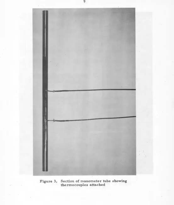
For the purpose of measuring the temperature at several points along

the manometer column, several chromel-alumel thermocouples were attached

to the surface of the inconel tube. The thermocouples used were made

from standard #24 chromel-alumel thermocouple wire with a guaranteed

accuracy of± 4°F from 0 to 530°F and± 3/4% from 530 to 2300°F. The

junction was formed by melting the two wires into a bead. This bead was

spot-welded to the surface of the inconel tube and the bead was then

ground down to minimize the surface defect. Figure 3 is a photograph

of a 3/8 inch tube with thermocouples attached similarly to those on

the manometer column.

The temperatures from the thermocouples were recorded on a twelve- ·

point Brown recorder with a 0-500°C scale. Since 24 thermocouples were

used on the system, each recorder point recorded alternately two specific

thermocouples. The calibration of the recorder was checked with a

poten-tiometer both by calibrating the recorder and by reading the emf of the

thermocouples periodically on .the potentiometer.

Simpson voltmeters and ammeters were placed in the circuit to measure

the power inputs to each heater. These meters were calibrated with a

Westinghouse type TA power analyzer.

Figure 4 is a photograph of the apparatus used including the auxiliary

i"

INCONEL TUBE

5

II

32

INCONEL TUBE

ALUNDUM BEADS

SINGLE WIRE HEATER

THERMOCOUPLE WELL

(

~

11

1NCONEL

TUBE)

PIPE

~

11

_1NCONEL

TUBE

PIPE HEATER

[image:16.602.107.531.115.647.2]

Figure 3. Section of manometer tube showing

[image:17.603.31.585.54.708.2]

[image:18.603.45.562.59.674.2]

IV. GENERAL THEORY

If the heat transfer in the manometer column is assumed to be due

solely to conduction, the temperature distribution in the column can be

determined from the general heat conduction equation which is given by

Schneider

(4)

as

Ill

q

K

=

a

au

at

( 1)

For a heat conducting medium in which there are no heat sources or heat

...

sinks, the term _!_ becomes zero. For a steady state or time independent

K

solution, the term

JL

au

also vanishes leaving the heat conduction

equa-a

at

tion in the form of Laplace's equation

(2)

Laplace's equation may be expressed in cy 1 i nd rIca 1 coordinates for

the case under consideration which is given as

c31

u

+

- -

au

+

c32

u

₌

0

(3)

dr

2

_r

or

az

2

where r is the radial variable and z is the longitudinal variable.

The solution of the Laplace equation is obtained ,by the technique

of separation of variables. The solution of the temperature as a function

the variable z, are obtained and are solved independently.

(5)

+

(6)

r

Equation 5 has the form of the wave equation which has a general

solution

Z(z)

=

A cos

/3

z

+

8 sin

/3

z

( 7)

Equation 6 has the form of the modified Bessel's equation which has a

solution of the form

(8)

The complete general solution for the temperature distribution In

a finite hollow cylinder Is obtained by substituting equations

7

and 8

u(r,z)

=

[Acos

/3z

+

B sin/3z] [ C

l

0

(~r)

+

D K

0

(/3r>]

(9)

The particular solution of this equation Is determined by applying the

existing boundary conditions and obtaining values for the constants A,

B, C, D, and ~ • The following section discusses the assumptions and

deviation of about± 0.1 em. Therefore, It will be sufficient to

main-taln the error in the measurement of pressure which Is due to the

uncer-talnty In the value of the density of the sodium to a similar magnitude

of± 0.1 em of sodium.

The density of sodium as a function of temperature Is given by

Sittig (5) as

( 1 0)

This equation is stated by Sittig to be valid to about± 0.20% for

tempera-tures up to 640°C. The rate of change of density with temperature Is

obtained from the derivative of equation 10.

=

- 2. 2 3

X

10-

4 _{- ( 11)}

Since the density of sodium varies nearly linearly with temperature In

the range being considered, i.e., 100-500°c, the average rate of change of

density with temperature in this range is approximately that at 350°C. At

the temperature of 350°C the rate of change of density Is -2.35 x lo-4

of 0.08688 gm/cm2 • Therefore, the product of the sodium height, the

a

uncertainty In the temperature, and~ must be less than 0.08688

au

gm/cm2 In order that the error be less than 0.1 em. This may be ex-pressed as

h

t.u

(2.35

x

1o·•

>

<

0.08688

( 12)

or

hllu

<

370

( 13)

Since the maximum sodium height which can be measured is about 100 em., the uncertainty In the temperature must be less than 3.7°C to Insure that the error due to the uncertainty in the density is less than the error due to the measurement of the sodium level.

The transfer of heat in the vertical direction of the manometer column is due mainly to the sodium. The heat transfer up the column by

the lnconel tubes and the alundum Insulators Is small and Is taken Into account by using an equivalent area for the sodium. The equivalent sodium area Is determined by determining the ratio of the total heat conducted

by the complete manometer column and that conducted only by the sodium.

The one dimensional heat conduction equation is given by Schneider

(4)

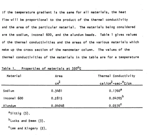
as

of the thermal conductivities and the areas of the various materials which make up the cross section of the manometer column. The values of the thermal conductivities of the materials In the table are for a temperature

Table 1. Properties of materials at 350°C

Material

Sodium lnconel 600 Alundum

8_{Sittig (5).}

blucks and Deem (3). clee and Kingery (2).

Area cm2

0.3481 0.2815 0.04048

Thermal Conductivity

cal/cm2_-sec-°C/cm

0.1760a 0.04705b 0.0370c

of 350°C which Is approximately the average of the temperatures being con-sidered. The heat flow In the vertical direction of the sodium Is given by

q

[image:24.601.85.560.75.507.2]

The total heat flow In the vertical direction of the manometer column

is given by

q

( 16)

The value obtained from equation 15 for the heat flow only in the sodium

~1.1.7

is O.OS&it cal/sec-°C/cm and the similar value for the complete manometer

column obtained from equation 16 is

0.~

cal/sec-°C/cm. The equivalent

area of sodium necessary to transfer the same amount of heat as the

com-plete column is found by multiplying the ratio of the heats by the actual

sodium area. The equivalent area has a value of

0.~

cm2 which

cor-responds to an annulus with an inside radius of 0.1981 em and an outside

radius of 0.4188 em. The error introduced in the heat flow by using this

equivalent area of sodium is a maximum of about 3.5% at both 100 and 500°C.

The basic assumption has been made that the transfer of heat by the

sodium is due entirely by conduction. This assumption should not introduce

much error since the size of the annulus is quite small which would tend

to eliminate any convection.

Using the previous assumptions, the following boundary conditions

can be used to determine the values of the constants in equation 9 which

is the general solution of the heat conduction equation.

1.) The plane at the base of the manometer column (z

=

o) is an

infinite heat source with a temperature which corresponds to

4.)

The heat flux out of the sodium at r a R Is equal to the heat

loss to the atmosphere which Is a function of the temperature

of the column.

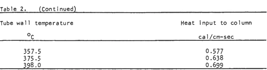
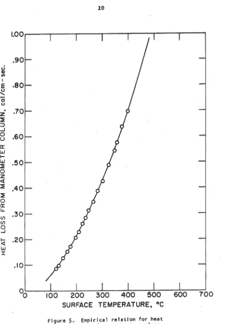
In boundary condition 4 the relationship between the heat loss to the atmosphere and the temperature of the manometer column was determined empirically. The results are shown in Table 2 and the curve of heat loss from the manometer tube per centimeter of length vs. temperature is shown In Figure

5.

Table 2. Heat Input to manometer column Tube wall temperature

120.5

130.5

148.5

164.0

177

.o

196.5

209.5

223.0

234.5 247

.o

265

.o

28~

.o

301

.o

324.5

347

.s

[image:26.591.108.522.107.297.2]

Table 2. (Continued)

Tube wall temperature

357.5 375.5 398.0

Heat input to column

cal/cm-sec

0.577 0.638 0.699

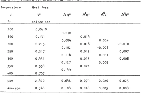
The equation for the curve can be expressed as a polynomial. The

degree of the polynomial which fits the experimental data is determined by

the method of differences as described by Sokolnlkoff and Redheffer (6).

The heat loss from the manometer tube at 50°C Intervals is obtained from

the experimental curve and tabulated in Table 3. The first, second,

third, and fourth forward differences are also shown in Table 3. Since

the smallest value of the sum of the terms divided by the number of terms

is for

6

3 _{q11 , the polynomial to be used is a second degree polynomial.}

( 17)

The constants in equation 17 were determined by applying a least squares

fit to the data In Table 2. The least squares fit ts obtained by requiring

that S be a minimum where S is defined as

S

=

.I [

f(u

1) -r•l

( 18)

[image:27.601.90.542.100.220.2]

[image:28.604.92.533.53.688.2]

I

e

u ...

-

0 u

.

z

~ ::::> _J 0

u

0::

w

~

w

~ 0

z

ct ~ ~ 0 0:: u.. (/) (/) 0 ..J

~

w

J:

.20

.10

100

500

SURFACE TEMPERATURE, °C

Figure

5

.

Empirical relation for heat

loss from manometer column

( 19)

The minimum value of S is obtained by setting the partial derivatives

Table 3. Forward differences for heat loss

Temperature Heat loss

u

q"

6

q"

f:lzq••

fl'q•• f:l.q ..

oc cal/cm-sec

100 0.0610

0.070

150 0.131 0.014

0.084 0.004

200 0.215 0.018 -0.010

0.102 -0.006

250 0.317 0.012 0.007

0.114 0.001

300 0.431 0.013 0.008

0.127 0.009

350 0.558 0.022

0.149

400 0.707

Sum 2.420 0.646 0.079 0.020 0.025

Average 0.346 0.108 0.016 0.005 0.008

of S with respect to b1, b2 , and b3 equal to zero. The following three

equations are obtained and solved simultaneously for b 1, b2 , and b3

using values from Table 2.

n

+

b

3

I

u~

=

(20)

[image:29.603.87.551.233.537.2]

b

LU~

=

31•1 I

fu

q

f•l I r

Using values obtained from these equations, equation 17 becomes

(23)

The complete solution of the general heat conduction equation can now be obtained using the assumptions and boundary conditions previously discussed. The general heat conduction equation for a medium with no heat sources or sinks and for steady state conditions is given by Laplace's equation

(2)

The first two boundary conditions are

u(r,O)

=

TL

(24)

For simplification In solving equation 2 for these boundary conditions,

the following substitution is made

w(

r, z )

=

u ( r , z) -

TL

(26)

The boundary conditions in equations

4

and

5

applied to the variable

w{r,z) give

w(r,O)

=

0

{2 7)

(

ow(r,z~

=

0

a

z

Jz=L

{28)

The heat conduction equation sti 11 has the form of Laplace's equation.

{29)

The Laplacian operator in the form of cylindrical coordinates is given by

+

r

aw

or

+

=

0

(30)

By applying the technique of separation of variables, the solution of this

equation will have the form

_..!__

a

1

_R(r)

+

₁

_aR(r)

+

_{.J_}

_{a•z(z) •}

0

<32 )

R(r)

a

r

2

_rR(r)

a

_r

_Z(z)

a

_z

1

Since a variation of z has no effect on the first two terms of this

equation and a variation of r has no effect on the third term, both the

first two terms and the third term must be constant. Since their sum Is

equal to zero, the value of the third term must be the negative of the

value of the first term. The boundary conditions specified by equations

27 and 28 require that this constant be real and positive as used in the

following equation.

I

a'R(

r)

-R-(r-) ar

1

+

a

R(r)

rR(r)

ar

(33)

The two separate differential equations obtained from equation 33 are

+

~

1

Z(z)

=

o

(34)

+

dR(r)

Equation 35 has the form of the wave equation which has a solution

of the form

Z(z)

=

A'cos~z

+

B'slnPz

(36)

Applying the boundary conditions given by equations 27 and 28 one

obtains

Z(O)

=

0

( oZ(z) \

=

0

oz

/z=L

.

. .

.

.

.

A'= 0

8',8cos/3L

=

0

Avoiding the trivial solution of

s

1 : 0 one is left with

(37)

(38)

cos

,8

L

=

0

09)

which gives

=

(2n-l),.

_2L

n=l 2 3 ···

'

'

'

{40)

solution for this equation is given by Schneider (4) as

(42)

The complete solution Is obtained by substituting equations 41 and 42

into equation 31. The constants are combined leaving only two unknown

constants fQr the remaining two boundary conditions.

w (

r,z)

(43)

The boundary condition at the Inside surface of the annulus, (I .e. r • P)

Is that the heat flux thru the wall Is constant at any point along the

column. This Is given by the one dimensional heat conduction equation

q

₌

- K

A c}tJ

N".

ar

(44)

In which q(P,z) • consta~t which Is equal to the heat Input of the

mano-meter heater per unit length. The thermal conductivity of sodium Is

given by Sittig (5) as a linear function of temperature

Since the substitution of u:w+TL was made to simplify the solution, the

thermal conductivity of sodium in terms of w Is

+

+

(46)

The heat flux Into the sodium at P per unit length of column is given by

I

q

= -

q

L

(47)

The partial derivative of equation

43

with respect to r is

(48)

For simplification in writing the equations in the remainder of the

derivation the following forms will be used

(49)

where F, f may represent H, h; M, m; or N, n and g may represent r, R,

or P. The following substitution wi 11 also be made

C

_

I

+

I

+

I

+

I (SO)

hmn-2h-2m•2n-l 2h+2m-2n-l 2h-2m-2n•l 2h+2m+2n-3

Using these simplifications, substituting equations

43, 46,

and

48

into

~m•l

a

This equation can be simplified by obtaining an orthogonal set of

equa-tlons from the Infinite series In the second term. If this equation Is

multiplied by the factor sin hz and the resulting equation Integrated

over the length of the column from z • o to z •

L.

the following set

of h equations are obtained where h

=

11 2.

3.

---2h-l

(52)

The boundary condition at r : R is given by q" : f{u) where f(u) Is the

function of the heat loss of the column and Is given by ~quatlons 17 and

23. Using equation 47 and making the proper substitutions gives

b

1

+

b

2

TL

+

b

3

T~

+ [

b

2

+

2 b

3

TL]

w

+

b

3

w

1

= -

2,. R [

a

1

+

a

2 TL

+

a

2

w ] : ;

(53)

Substitution of equations 43 and 48 Into this equation gives the complete

01) 01)

+

b

₃

2: 2:

N

lR)M

CR)sinP, z

sin~ z(54)

n=lm=IU .. '0 n m

oom

+

2,.Ra

₂

2: 2:

NcJR)M

1

(R)sin~nz sin~mz

=

0

n=l m:l

As was done for equation 51, this equation is multiplied by the factor

sin~hz and integrated over the interval of z from 0 to L. This gives another set of equations which contain a double infinite series.

(55)

Equations 52 and 55 were solved simultaneously to determine Ah and Bh. Since these two equations contain double infinite series, the solution for the values of'Ah and Bh were obtained on a computer by an iterative process. In the two final equations for Ah and Bh, i.e., equations 52 and 55, the contribution of the series is small compared to the other terms in the equations. A fair approximation of Ah and Bh can be obtained by omit-ting the series terms and solving the two equations simultaneously. The approximation for Ah and Bh can be improved by using the previously de-termined values of Ah and Bh in the series terms and then solving the remainder of the equation for Ah and Bh again. This process can be re-peated until the desired accuracy of Ah and Bh is obtained.

a2: •1 .16 X 10•4

bl

=

-0.0272 b2: 5.84 X 10•4

b

₃

=

3 •

12 x 1

o-6

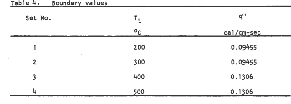
A separate set of values for Ah and Bh were obtained for each value of

simulated loop temperature, TL• and each value of heat loss from the manometer column, q11 _• The four sets of boundary values listed In

[image:38.597.77.548.55.331.2]

Table 4 were used for the calculations.

Table 4. Boundary values

Set No. _TL qll

oc cal/cm-sec

200 0.09455

2 300 0.09455

3 400 0.1306

4 500 0. 1306

Only the first twenty values of Ah and Bh were solved and these are shown in Tables 6 and 7.

[image:38.597.65.530.432.599.2]

dlstribu-tlon, u(r,z}, was then obtained by substituting equation

43

Into equation

26. The values of the temperature obtained from this equation at the

Periodically throughout the runs the temperatures of the recorder were

checked against those read by the potentiometer. The ammeters and

volt-meters used for measuring the power input to the heaters were checked

against a power analyzer before and after the run.

After the sodium was molten, it was forced into the manometer column

from the reservoir by pressurized helium. A pressure difference of about

1 3/4 psi between the reservoir and the top of the manometer column

pro-duced a column of sodium approximately 120 em.

The first part of the experiment consisted of determining the

rela-tionship between the heat loss from the manometer column and the

tempera-ture of the column. This was achieved by setting the heaters to obtain a

constant temperature along the manometer column and determining the power

input to the manometer column by reading the voltage and current to the

manometer heater. The temperatures of the column were obtained from the

thermocouple recorder by averaging the temperatures over five recorder

cycles. The recorder printed the temperature at 24 points In a period of

six minutes. This allowed enough time to assure that the temperature had

reached steady state conditions. These measurements were made at column

temperatures ranging from 100 to 400°C and the results are shown in Table

2 and Figure

5.

The principal part of the experiment consisted of measuring the

of the sodium In the pipe at the bottom of the manometer column was at

a higher temperature than that In the column. This was done by setting

the current to the manometer heater to the value obtained from Figure

5

which would give the desired manometer column temperature. The reservoir

and pipe heaters were then turned up to give a desired higher temperature.

The temperatures at the points along the manometer column were obtained

in a manner similar to that used in the first part of the experiment.

Since the experimental measurements were taken on the outside of the mano-meter tube and the theoretical values were calculated for the outer

sur-face of the sodium, the temperature drop across the tube wall Is not

taken into consideration In the comparison of the experimental and theoretical data. This temperature difference can be shown to be small

in the temperature range being considered by calculating the temperature

drop across the tube wall at some mean temperature using the one

dimen-slonal heat conduction equation.

q

L

= -

21r

K

c3r

c3u

(54)

For a mean temperature of 400°C which is in the upper part of the

tempera-ture range being considered, and using the following set of values for the

. calculations, the temperature drop across the 35 mil tube wall is less

than one-half of one degree centigrade.

q/L • 0.705 cal/cm-sec

K - 0.0490 cal/cm2_-sec-°C/cm

r₀ - 0.476 em

r· _I

=

0.387 em

The four plots of temperature vs. position along the manometer column show relatively good agreement between the experimental points and the

!

_.

TL ·zoo•c

Tc •125 •c

q' •0.094&& CAL/cM ... SEC.

- THEORETICAL CURVE

o EXPERIMENTAL DATA

OL---~----~---~----~----~---~---L----~ 100

[image:43.601.97.495.78.677.2]

TEMPERATURE , • C

Figure

6.

Temperature gradient along manometer column for Setting No. 1

3

1~0 200

TL •300

•c

Tc •12S •c

q• •0.094SS CALICM.•SEC.

- THEORETICAL CURVE

o EXPERIMENTAL DATA

2!50 300 3SO TEMPERATURE •

•c

400 4~0

Figure ]. Temperature gradient along manometer column for Setting No. 2

[image:44.598.87.502.60.665.2]

TL • 400•c

Tc • 1so•c

q' •0.1306 CAL'cM.·SEC.

- THEORETICAL CURVE

o EXPERIMENTAL DATA

[image:45.597.107.518.50.670.2]

TEMPERATURE :c

z

2

~

u7

150 200

TL •500

•c

Tc

•150

•c

q I •0.1306CALyCM.- SEC.

- THEORETICAL CURVE

o . EXPERIMENTAL DATA

250 300 350

TEMPERATURE,

•c

[image:46.595.107.507.63.678.2]

400

Figure

9.

Temperature gradient along manometer column for Setting No. 4

appear at the low end of the column at the elevation two, seven, and

twelve centimeters. The experimental temperatures are all lower than

the theoretical values at these points. The difference at the two

centimeter elevation is quite large. Since the other measurements

agree, it is believed that this measurement was too close to the cross

pipe to give an accurate temperature indication. The average permissible

error in temperature was previously calculated to be about 3.7°C. The

agreement between the theoretical and experimental values is within this

allowable error over most of the column length and the average error

series to series of twenty terms and using the iterative method for

cal-culating Ah and Bh, were apparently satisfactory. The last iteration

changed the values of Ah and Bh by less than 0.05% in all cases except

for A1 of run

4.

The change was only slightly greater in this case. It can be concluded, therefore, from the results of this

investiga-tlon that the theoretical procedure used here may be used to determine

the temperature distribution within the stated accuracy for loop

tempera-tures from 200 to 500°C and for column temperatempera-tures of 125 to 150°C.

In this investigation the assumption was made that the level of the

sodium in the manometer column was alwa~s considerably above the level

at which the temperature gradient in the z direction became zero. Further

studies could be made on the theoretical solution of the problem in which

the sodi4m level is below the point at which the temperature gradient

along the column becomes zero. This problem would involve a change in

the boundary condition at z : L which in this case was

(55)

IX. LITERATURE CITED

1. Cars law, H.

s.

and Jaeger, J, C. Conduction of heat in solids.

2nd ed. London. Oxford University Press. 1959.

2. Lee, D.

w.

and Kingery, W. D. Radiation energy transfer and thermal

conductivity of ceramic oxides. J. Am. Ceram. Soc. 43, No. 11:

595~605. Nov. 1960.

3.

Lucks,

c.

F. and Deem, H.

w.

Thermal properties of thirteen metals.

ASTM special technical publication No. 227. 1958.

4.

Schneider, P. J. Conduction heat transfer. Cambridge, Mass.

Addison~Wesley Publishing Co., Inc. 1955.

5.

Sittig, Marshall. Sodium, its manufacture, properties, and uses.

6.

New York, N.Y. Reinhold Publishing Corp. 1956.

Sokolnikoff, I.

s.

and Redheffer, R. M.

and modern engineering. New York, N. Y. 1958.

TL : 400

em

_{TL • 200}

\ . 300

TL : 500

1

2.0

178.8

252.6

316.0

386.6

2

7.0

151 • 2

188.4

226.4

256.0

3

12.0

138.8

155.5

192.4

200.8

4

17

.o

132.8

142.2

169.4

174.0

5

22.0

128.2

134.6

160.2

162.8

6

27.0

126.5

130.2

156.2

157

.a

7

32.0

125.8

127

.a

153.6

.

154.8

8

37.0

125.8

127

.o

152.2

153

.o

9

42.0

124.0

125.2

150.4

151 • 0

10

47.0

124.0

124.6

149.6

149.5

11

52.0

125.8

126.2

150.4

150.4

1 2

57.0

126.6

126.8

151 • 6

151 • 2

13

62.0

125.5

125.8

150.2

150.2

14

67.0

125.6

126.0

150.2

150.2

15

72.0

125.0

125.6

150.0

150.0

16

77.0

125.5

125.6

150

.o

150.2

17

82.0

124.2

124.6

149.4

149.8

18

87.0

124.6

125.6

150.2

151

.o

19

92.0

124.2

125.0

149.8

150

.o

20

97.0

124.0

124.8

149.4

150.0

[image:50.595.61.522.81.563.2]

Table 6.

Values of Ah

h

TL : 200

_{\ =}

300

TL : 400

T : 500

L

1

-94.46

-220.2

-315.1

-440.6

2

-28.18

-66.18

-96.10

-135.1

"

-14.02

-33.34

-49.49

-70.23

~·

4

-8.000

-19.33

-29.36

-42.13

. 5

_-4.927

_-12.11

_-18.78

_-27.28

6

-3. 211

-8.026

-12.68

-18.63

7

-2.191

-5.563

-8.925

-13.26

8

-1.553

-3.998

.

-6.501

-9.760

9

-1 • 136

-2.962

-4.870

-7.381

10

-0.8538

-2.250

-3.736

-5.709

11

-0.6556

-1.746

-2.924

-4.501

12

-0.5149

-1 .379

-2.327

-3.606

13

-0.4107

-1 • 1 07

-1 .880

-2.930

14

-0.3326

-0.9012

-1.538

-2.409

15

-o.

2728

-0.7422

-1.273

-2.001

16

-0.2264

-0.6177

-1 .063

-1.678

17

-o

.1897

-0.5188

-0.8956

·

-1 .417

18

-o.

1605

-0.4392

-0.7600

-1.205

19

-o.

1368

-0.3745

-0.6491

-1 .030

[image:51.598.104.542.144.504.2]

h

\ =

₂₀₀

_{TL :}

₃₀₀

_{TL :}

₄₀₀

T L :

500

1

0.09442

0.09376

0.1314

0. 1309

. 2

_.03054

_.02904

_.o4o68

_.03920

3

.01750

.0154o

.02145

.01925

4

.01190

.009500

.01302

.01035

5

.008862

.006339

.008437

.005485

6

.006990

.004455

.005678

.002571

7

.00574o

.003252

.003904

.0007237

8

.004855

.002445

.002710

- .0004883

9

.004200

.001881

.001879

- .001301

10

.003697

.001475

.001284

- .001851

11

.003300

.001175

.0008509

- .002224

12

.002979

.0009485

.0005297

- .002474

13

.002715

.0007748

.0002886

- .002637

14

.002494

.0006391

.0001056

- .002737

15

.002305

.0005315

.00003443

- .002791

[image:52.600.76.530.158.533.2]

Table 8.

Theoretical results

Position

Temperature, oc

Along Column

em

TL : 200

TL : 300

_{\ =}

400

TL : 500

1.0

191 .4

278.7

367.2

451 .9

2.0

183.2

258.5

335.9

406.4

3.0

175.7

240.1

307.9

365.7

4.0

169.0

224.0

283.7

331

.o

5.0

163.4

210.5

263.8

302.9

7.5

152.9

186.5

229.8

256.2

10.0

145.7

170.4

208.0

227.4

12.5

139.9

157.4

190.4

203.6

15.0

135.6

147.8

177.4

185.8

20.0

131

.o

137.8

165.2

170.4

25.0

128.0

131 • 2

156.7

158.8

30.0

126.8

128.8

154.4

156.2

35.0

125.9

126.6

151 • 5

152.2

40.0

125.6

126.3

151.5

152.5

50.0

125.3

125.5

150.7

1 51 • 5

60.0

125.2

1 25.3

150.5

151.2

70.0

125.2

1 25.2

150.4

151 • 1

80.0

125.2

1 25.2

150.4

151 • 1

90.0

1 25.1

1 25.2

150.4

151

.o

[image:53.587.80.518.155.541.2]