Performance Analysis of Tracking on Mobile Devices using Local Binary Descriptors

(1)

Rochester Institute of Technology

RIT Scholar Works

Theses Thesis/Dissertation Collections

5-2014

Performance Analysis of Tracking on Mobile

Devices using Local Binary Descriptors

Mohammad Faiz Quraishi

Follow this and additional works at:http://scholarworks.rit.edu/theses

This Thesis is brought to you for free and open access by the Thesis/Dissertation Collections at RIT Scholar Works. It has been accepted for inclusion in Theses by an authorized administrator of RIT Scholar Works. For more information, please [email protected].

Recommended Citation

(2)

Performance Analysis of Tracking on Mobile Devices

using Local Binary Descriptors

by

Mohammad Faiz Quraishi

A Thesis Submitted in Partial Fulfillment of the Requirements for the Degree of Master of Science in Computer Engineering

Supervised by

Dr. Andreas Savakis

Department of Computer Engineering Kate Gleason College of Engineering

Rochester Institute of Technology Rochester, NY

May 2014

Approved By:

_____________________________________________ ___________ ___

Dr. Andreas Savakis

Primary Advisor – R.I.T. Dept. of Computer Engineering

_ __ ___________________________________ _________ _____

Dr. Andrés Kwasinski

Secondary Advisor – R.I.T. Dept. of Computer Engineering

_____________________________________________ ______________

Dr. Roy Melton

(3)

Dedication

I would like to dedicate this thesis to my parents, Dr. Abdul Rashid Quraishi and Wasima

(4)

Acknowledgements

I would like to express my thanks and appreciation to my advisor, Dr. Andreas Savakis

for all his assistance and support in my research. I would also like to thank Dr. Andrés

Kwasinski and Dr. Roy Melton for serving on my committee. I would also like to express

my gratitude to all the staff of the Kate Gleason College of Engineering Computer

Engineering Department for all assistance and work during my studies. Lastly, I would

like to thank all my lab colleagues who have helped not only in collaboration but also in

(5)

Abstract

With the growing ubiquity of mobile devices, users are turning to their

smartphones and tablets to perform more complex tasks than ever before. Performing

computer vision tasks on mobile devices must be done despite the constraints on CPU

performance, memory, and power consumption. One such task for mobile devices

involves object tracking, an important area of computer vision. The computational

complexity of tracking algorithms makes them ideal candidates for optimization on

mobile platforms.

This thesis presents a mobile implementation for real time object tracking.

Currently few tracking approaches take into consideration the resource constraints on

mobile devices. Optimizing performance for mobile devices can result in better and more

efficient tracking approaches for mobile applications such as augmented reality. These

performance benefits aim to increase the frame rate at which an object is tracked and

reduce power consumption during tracking.

For this thesis, we utilize binary descriptors, such as Binary Robust Independent

Elementary Features (BRIEF), Oriented FAST and Rotated BRIEF (ORB), Binary

Robust Invariant Scalable Keypoints (BRISK), and Fast Retina Keypoint (FREAK). The

tracking performance of these descriptors is benchmarked on mobile devices. We

consider an object tracking approach based on a dictionary of templates that involves

generating keypoints of a detected object and candidate regions in subsequent frames.

Descriptor matching, between candidate regions in a new frame and a dictionary of

templates, identifies the location of the tracked object. These comparisons are often

(6)

Google’s Android operating system is used to implement the tracking application

on a Samsung Galaxy series phone and tablet. Control of the Android camera is largely

done through OpenCV’s Android SDK. Power consumption is measured using the

PowerTutor Android application. Other performance characteristics, such as processing

time, are gathered using the Dalvik Debug Monitor Server (DDMS) tool included in the

Android SDK. These metrics are used to evaluate the tracker’s performance on mobile

(7)

List of Figures

Figure 1 BRIEF sampling patterns a-e... 6

Figure 2 BRISK sampling pattern... 9

Figure 3 FREAK sampling pattern ... 11

Figure 4 CAMSHIFT Flow Chart ... 13

Figure 5 TLD block Diagram ... 16

Figure 6 Android Operating System Architecture ... 21

Figure 7 Program Flow Chart ... 33

Figure 8 Search Pattern r=8, s=1 ... 34

Figure 9 Search Pattern r=8, s=2 ... 35

Figure 10 Software Block Diagram ... 38

Figure 11 Tracker Block Diagram ... 39

Figure 12 Options file syntax ... 42

Figure 13 Frame Rate by Search Radius Single Threaded ... 48

Figure 14 Frame Rate by Search Radius Multithreaded ... 48

Figure 15 Single Threaded Power Consumption based on candidates ... 50

Figure 16 Multithreaded Power Consumption based on Candidate Radius ... 51

Figure 17 Comparison of NEON Scoring ... 53

Figure 18 Comparison of Power Consumption ... 53

Figure 19 Frame Rates based on processing time per frame ... 55

Figure 20 Cliffbar Error with 441 Candidates ... 57

Figure 21 Average Tracking Error: Cliffbar Error with 289 Candidates ... 58

(12)

Figure 23 Average Tracking Error: Cliffbar Error with 81 Candidates ... 60

Figure 24 Cliffbar Frames 9, 30, 88, 157 ... 60

Figure 25 Average Tracking Error: Twinings 441 Candidates ... 62

Figure 28 Average Tracking Error: Twininigs 81 Candidates ... 65

Figure 29 Average Tracking Error: Twinings Frames 7, 111, 197 ... 65

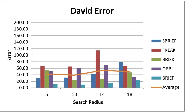
Figure 30 Average Tracking Error: David Error with 441 Candidates ... 67

Figure 33 Average Tracking Error: David 81 Candidates ... 70

Figure 34 David Frames 1, 11, 31... 70

Figure 35 David Frames 241, 323, 370, 396 409... 71

Figure 36 Average Tracking Error: Dollar 441 Candidates ... 72

Figure 40 Dollar Frame 58, 137, 203, 253 ... 75

Figure 41 Average Tracking Error: Coke 41 Candidates ... 77

Figure 43 Average Tracking Error: Coke 169 candidates ... 79

(13)

Figure 46 Average Tracking Error: Sylvester 441 Candidates ... 81

Figure 49 Average Tracking Error: Syslvester 81 Candidates ... 84

Figure 50 Sylvester Frames 18, 162, 369 ... 84

Figure 51 Average Tracking Error: Surfer 441 Candidates ... 85

Figure 55 Surfer Frames 401, 450, 552, 580, 718 ... 88

Figure 56 Average Tracking Error: Toni Candidates ... 90

Figure 57 Average Tracking Error: Toni 289 Candidates ... 91

Figure 60 Toni Frames 7, 21, 85, 120, 131, 241, 288 ... 94

Figure 61 Average Tracking Error: Dudek Error with 441 Candidates ... 96

Figure 65 Dudek Frames 16, 98, 206, 221, 375, 977 ... 99

Figure 66 Dudek Error with a radius of 44 ... 100

Figure 67 Dudek Error with a radius of 36 ... 101

(14)

Figure 69 Effect of varying sigma in Cliffbar Error ... 103

Figure 70 Effect of varying sigma in Coke Error ... 103

Figure 71 Cliffbar Scale Invariance ... 105

Figure 72 Twinings Scale Invariance ... 105

Figure 73 David Scale Invariance ... 106

Figure 74 Dollar Scale Invariance ... 106

Figure 75 Coke Scale Invariance ... 107

Figure 76 Sylvester Scale Invariance ... 107

Figure 77 Surfer Scale Invariance... 108

Figure 78 Toni Scale Invariance ... 108

Figure 79 Dudek Scale Invariance ... 109

Figure 80 Cliffbar Rotation Invaraiance ... 110

Figure 81 Twininigs Rotation Invariance ... 110

Figure 82 David Rotation Invariaince... 111

Figure 83 Dollar Rotation Invariaince ... 111

Figure 84 Coke Rotation Invariance ... 112

Figure 85 Sylvester Rotation Invariance... 112

Figure 86 Surfer Rotation Invariance ... 113

Figure 87 Toni Rotation Invariance ... 113

Figure 88 Dudek Rotation Invariance ... 114

Figure 89 Binary Descriptor comparison to CAMSHIFT ... 115

(15)

List of Tables

Table 1 Device Specifications ... 41

Table 2 Videos used for testing ... 41

Table 3 Percent of Time Per Frame used for Description ... 45

Table 4 CPU Percent of Time Per Frame used for Scoring ... 46

Table 5 Percent Difference from Mean among OpenCV Descriptors ... 49

Table 6 Percent Difference from the Mean frame rate ... 49

Table 7 Average Power Consumption by Candidate Radius ... 51

Table 8 Average Tracking Error: Cliffbar with 441 candidates ... 56

Table 12 Average Tracking Error: Twinings 441 Candidates ... 62

Table 16 Average Tracking Error: David 441 Candidate Points ... 66

Table 17 Average Tracking Error: David Error with 289 Candidates ... 67

Table 20 Average Tracking Error: Dollar 441 Candidates ... 72

(16)

Table 24 Average Tracking Error: Coke 441 Candidates ... 76

Table 28 Average Tracking Error: Sylvester 441 Candidates ... 81

Table 32 Average Tracking Error: Surfer 441 Candidates ... 85

Table 36 Average Tracking Error: Toni 441 Candidates ... 89

Table 40 Average Tracking Error: Dudek Error with 441 Candidates ... 95

Table 44 Change in Power and FPS for 1681 Points ... 116

(17)

(18)

Glossary

BRIEF Binary Robust Independent Elementary Features descriptor

BRISK Binary Robust Independent Scalable Keypoint descriptor

CAMSHIFT Continuous Adaptive Meanshift

Candidate radius The number of candidate points that make up the radius for the search

region

FREAK Fast Retina KeyPoint descriptor.

ORB Oriented FAST and Rotated BRIEF descriptor.

Sample radius The radius for the entire span of all candidate points.

SBRIEF Simple BRIEF

(19)

Chapter 1

Introduction

As mobile devices increase in ubiquity, so has the demand that they perform more

complex tasks. Whereas phones and tablets initially were used for calls and web surfing,

focus has now shifted to using these devices for applications such as video conferencing

and 3D gaming. Computer Vision presents another interesting opportunity for mobile

devices, as their form factor and popularity presents many interesting and novel

applications.

One of the most popular uses for mobile object tracking is augmented reality.

Mobile apps such as LayAR annotate frames from a mobile camera by tracking either a

marker or natural feature. Usually these applications are used for commercial purposes

that present content to supplement products or advertisements. In addition, mobile object

tracking can be used to assist those with low vision, as seen in [1]. Here a mobile

Android device superimposed faces found in a scene in areas where individuals affected

with blind spots or tunnel vision could see them. Billinghurst et al. all further show the

application of augmented reality in the classroom via mobile devices [2]. Both these

examples rely on efficient, accurate, and fast methods of tracking on mobile devices. Yet

another example for the importance of this work can be found in the work of Navab et al.,

who uses augmented reality to assist surgeons [3]. Although the system described by

Navab et al. does not use a mobile platform, advances in mobile tracking, could greatly

improve the usability and reduce the cost of computer vision in medicine.

In addition to good tracking performance, tracking on mobile devices must be

power conscious. Any application that significantly reduces the battery life of a mobile

(20)

Saipullah et al. note that even simple image processing tasks on mobile devices show

significant power consumption [4]. For this reason, any proposed mobile tracking

application must also use power consumption as a metric.

Previously, Wagner et al. presented a SIFT-based tracking model for mobile

phones in [5]. SIFT, or Scale Invariant Feature Transform, is a popular and robust

descriptor for image description, but is also very complex. In this work, we benchmark

binary descriptors that require only comparisons between pairs of pixels to describe a

keypoint. These descriptors are becoming increasingly popular, because they are not

patent protected like SIFT and are simpler to implement. Further, we use these

descriptors in our template based tracker to benchmark performance on mobile devices.

To our knowledge this is the first comprehensive implementation of object

tracking on a mobile device using binary descriptors. Our tracker has the ability to use

five commonly known binary descriptors and a custom light weight implementation of

BRIEF described in Section 4.1.1. Whereas some tracking work describes frame rate by

the observed processing time, our work contributes benchmarking data for these

descriptors in terms of their real world frame rate as measured on an Android

smartphone. In addition to this we also present benchmarking data on power consumption

for the description methods used in our tracker. Further, we show the effectiveness of our

tracking methodology to generate accurate results based on testing of standard videos.

This remainder of this work is organized as follows. Chapter 2 presents

background on well-known binary descriptors and other object tracking

methodologies. Chapter 3 describes the background of the Android technologies that are

(21)

measurements. Chapter 4 details our tracking algorithm and the software implementation

for the Android OS. In Chapter 5 we present our tracker’s performance results based on

frame rate, power consumption, accuracy and invariance to scale and rotation as well as a

comparison to other trackers. In Chapter 6 we conclude this thesis, summarize our

(22)

Chapter 2

Background

2.1. Binary Descriptors

In this chapter we describe the various binary descriptors to be benchmarked on

our mobile tracking system.

2.1.1 BRIEF

Binary Robust Independent Elementary Features, or BRIEF, was proposed by

Calonder et al. in 2010. BRIEF is an early binary descriptor that attempts to reduce the

complexity of histogram descriptors such as SIFT and SURF. Being a binary descriptor,

BRIEF represents a keypoint as a bit string generated from intensity comparisons from a

sampling pattern.

{ (1)

Given a pair of pixels from the sampling pattern, if a pixel is greater than a pixel

the corresponding bit, , is represented as a 1, or 0 otherwise. These comparisons are

performed for the number of times needed to fill the length of the descriptor. For

example, if we are using a 32 byte BRIEF descriptor, we need 512 sample points for 256

comparisons to comprise the 32 bytes. After this procedure, two descriptors can be

compared via calculating the Hamming distance between the bit strings.

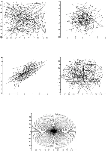
When generating the bit strings for the BRIEF descriptor we must have two

vectors of points for comparison. The BRIEF descriptor does not specify a sampling

pattern for the points in these vectors, and . Instead, Calonder et al. present five

(23)

Gaussian random samples, (c) Gaussian samples where points in are sampled with a

standard deviation of , where is the sample standard deviation, and points in are sampled with a standard deviation of , (d) random samples along a polar grid, and (e) sampling where takes on all values in a polar grid and all are . Using these patterns Calonder et al. show nearly similar recognition rate for all sampling

patterns, except with the final pattern which gives lower performance in all cases. The

quick comparisons and good recognition make BRIEF an interesting candidate for

benchmarking on a mobile device. The size of BRIEF can vary depending of

performance needs further making the descriptor more suitable for real time applications

(24)

[image:24.612.130.490.78.590.2]

Figure 1 BRIEF sampling patterns a-e

2.1.2 ORB

The Oriented FAST and Rotated BRIEF, or ORB, descriptor was proposed by

(25)

alternative to SIFT, intending to allow better performance in real time applications. The

ORB descriptor builds upon the FAST keypoint detector and the BRIEF descriptor [6].

The first step in the creation of ORB is adding an orientation component to the

FAST feature detector. FAST is a detector used for corners around the radius of a certain

keypoint [6]. Once this is completed the keypoints are threshold by a Harris measure to

produce corners. These corners are further used in a pyramid to create multi-scale

features.

Rublee et al. use an intensity centroid which assumes that a corner’s intensity is

offset from its center. In order to find the centroid, the moment of the patch is first

defined by Equation (2).

∑

(2)

Using Equation (2) the centroid can be found using Equation (3).

(

)

(3)

Using a vector from the corner to the center an orientation can be defined using the

quadrant aware version of arctangent, arctan2 [6]. This is shown in Equation (4).

(4)

This is the means by which the BRIEF descriptor is oriented for construction of the ORB

descriptor.

However, rather than using the same BRIEF descriptor described in [7], Rublee et

al. modified the sample points so that they have a high variance and are uncorrelated. In

(26)

five proposed distributions. However, these points may not have high variance and may

be correlated. The higher the variance between the sample points, the more descriptive

individual descriptors become [6]. Using a training set of images Rublee et al. were able

to determine a high variance pattern for the BRIEF component of the ORB descriptor.

The oriented FAST keypoint feature and the high variance BRIEF are combined to create

ORB.

Rublee at al. tested the ORB descriptor against SIFT and SURF for performance.

They show that computing ORB takes significantly less time than SIFT or SURF [6].

Because of its inexpensive computation in relation to SIFT and SURF, ORB is more

suitable for a mobile platform. Further, the authors of ORB implemented a real time

tracker on a mobile phone to test its ability to performance. Rublee at al. were able to

track at around 7 frames per second on a 640 by 480 pixel image.

2.1.3 BRISK

Binary Robust Invariant Scalable Keypoints or BRISK was proposed by

Leutenegger et al. in 2011 [8]. Unlike BRIEF, BRISK has a predefined sampling pattern

for generating the bits in the descriptor. These comparisons can be seen in Figure 2, as

short pairs forming a circular pattern. Short pairs of points are those with a distance

below a defined threshold; these are used for the description while longer pairs, those

with greater distance, are used for orientation information.

Unlike BRIEF, BRISK is designed to be rotation invariant. Rotation invariance

adds complexity to the description process, but allows better tracking of moving objects.

Orientation is first calculated using the gradient for a sample patch. Once this is done, the

(27)

that when an object is rotated, it should produce the same gradient as the original. Since

sampling is performed along the gradient, the bit string of the original and rotated

[image:27.612.176.435.157.419.2]

keypoint should be the same making BRISK invariant to rotation.

Figure 2 BRISK sampling pattern

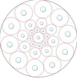
2.1.4 FREAK

The Fast Retina Keypoint, or FREAK, descriptor was proposed by Alahi et al. in

2012 [9]. The FREAK descriptor is 64 bytes long and has the option of rotation and or

scale invariance. The motivation for FREAK was to create a sampling pattern that

emphasized robust performance. As seen in the previous sections, there are many ways to

choose the sampling pattern for a binary descriptor. Rather than turning to random

sampling as in the case of BRIEF, or concentric circles as in the case of BRISK, the

(28)

The FREAK descriptor’s most unique feature is that its sampling pattern attempts

to mimic the human retina. In the human eye, photoreceptors influence ganglion cells that

ultimately create the receptive field [9]. Alahi et al. note that the distribution of ganglion

cells decreases exponentially with their distance away from the fovea, while the size and

dendritic field increases with distance from the fovea. Using this as inspiration, the

FREAK descriptor uses a circular sample grid around a keypoint, with decreasing density

proportional to the distance from the keypoint. As in BRISK, different kernel sizes are

used for every sample point. However, in order to follow the retinal model, the standard

deviation of the Gaussian kernel is based on the four regions of the eye: foveola, fovea,

parafoveal, and perifoveal. As the sample points grow further away in distance from the

center, so does the standard deviation of the Gaussian kernel. In addition to this, FREAK

uses overlapping receptive fields when sampling, whereas BRISK’s sample points do not

overlap. Alahi et al. note that using overlapping fields increases accuracy, possibly

because more information is captured. This adds redundancy and discriminative power

[9]. The final descriptor is calculated with comparisons over pairs of receptive fields

defined by Equation (5) and Equation (6).

∑

(5)

{ ( ) ( )

(6)

In Equation (6) is a pair of receptive fields, is the desired length of the descriptor,

and ( ) is the intensity of the first field of the pair, [9]. After generation, the FREAK descriptors can be compared using the Hamming distance, as with any other

(29)

Alahi et al. note that humans do not look at a scene steadily. Rather the human

eye performs a saccadic search that moves from lower detail of the perifoveal area to the

most detailed region, the foveola. Using this formula the eye can make easy estimates of

the locations for objects before using more detailed information. The FREAK descriptor

is designed to work the same way cascading information in a coarse to fine pattern. This

means that coarse comparisons are stored at the beginning of the bit string, while finer

ones at the end. In practice Alahi et al. state that more than 90% of potential candidate

points can be discarded by comparing just the first 16 bytes of the 64-byte FREAK

descriptor. This feature makes the descriptor attractive on a mobile platform, as it can

greatly reduce the amount of comparisons needed to be performed in real time.

Peri

Para

Fovea

Figure 3 FREAK sampling pattern

2.2. Other Description Methods

Here we describe image description and tracking using methods other than binary

(30)

2.2.1 Continuous Adaptive Mean Shift (CAMSHIFT)

Another popular tracking method is Continuous Adaptive Mean Shift or

CAMSHIFT and is described in [10] by Bradski. CAMSHIFT uses a histogram of

hue-saturation-value (HSV) values to describe a patch.

An initial region is selected that represents the object to be tracked. From this

patch, a color histogram is created from the hue values. This histogram is then used to

create a probability distribution for the different hue values for the region that is tracked.

For each subsequent frame, the probability distribution is used to find the center of mass

within the search window. After finding the center of mass, the search window is

centered at that point and the mass under it is updated. After this, convergence is tested.

If the distributions converge, the location of the search window is reported as the new

location for the object. The search window is then updated and set it as the starting

calculation for the subsequent frames. If convergence fails, CAMSHIFT continues

searching until we find a convergent region set by a threshold. A flow chart of the

CAMSHIFT algorithm can be found in Figure 4.

Although CAMSHIFT is a simple and effective algorithm, it is not very robust

since it depends on the hue of the object being tracked. This means that objects with

similar hue may be learned as tracking continues. In addition to this, since CAMSHIFT

(31)

Choose initial search window

Set Calculation

region

Use (X,Y) to set search

window center

Color histogram look-up in calculation

region

Color probability distribution

Find Center of mass in search window

Center search window at center

of mass

Converged?

No

Report X, Y,

Z, and Roll Yes

HSV Image

Figure 4 CAMSHIFT Flow Chart

In previous work, CAMSHIFT was used to extend the work in [1]. The

CAMSHIFT algorithm was chosen as a fast method to track human flesh tones for low

(32)

but was highly susceptible to drift because of CAMSHIFT’s color dependence. A

comparison to this method can be seen in Section 5.12.

2.2.2 Multiple Instance Learning (MIL)

The MIL or Multiple Instance Learning tracker was first proposed by Babenko et

al. in [11]. The MIL tracker is designed to track an object by learning from multiple

positive and negative examples. This is done by a boost algorithm called

Online-MILBoost which uses many weak classifiers to generate one strong classifier as seen

Equation (7).

∑

(7)

The MIL algorithm works by bagging positive and negative examples into several bags.

A bag is deemed to be a positive bag if it contains at least one positive example, whereas

all other bags that do not contains one positive example are labeled negative. However,

the images within each bag are not labeled.

At the beginning, a set of image patches are cropped out from the previously

known location within some search radius. The cropped images can be defined using the

following equation.

‖ ‖ (8)

In Equation (8) where is the location of a patch , and is the object location at time . The MIL classifier is then used on these patches to find the patch with the highest

probability of being the object and that is decided as the next location. After this is done,

(33)

newly determined location within some radius. These patches are defined using Equation

(9).

‖ ‖ (9)

These patches are placed into the positively labeled bag. Negative samples are placed into

bags as well by cropping out patches defined as by Equation (10).

_‖ _‖ ₍₁₀₎

A random subset of these negative patches is taken if the set is too large and placed into

its own negative bag. Once these bags are produced they are used to retrain the MILBoost

algorithm, for which details are described in [11].

Babenko et al. test the MIL tracker on several standard videos and present their

results for the online boosting method. The MIL tracker was shown to have either the

lowest or second lowest error from ground truth in all videos tested [11].

2.2.3 Track-Learn-Detect (TLD)

The TLD or Tracking-Learning-Detection tracking is another approach to

tracking that does not use binary descriptors. TLD was proposed by Kalal et al. in [12], as

a means to combine the strengths and weakness of detection and tracking into a long term

tacking approach. Detectors are designed to run every frame and do not drift as a trackers

do. Furthermore a detector not only can give the position of an object, but also can be

used to determine if an object is no longer in a frame or occluded. However, a detector

requires training beforehand to operate and often does not perform as fast as a tracker.

Although a tracker is faster, it can drift due to accumulation of error and will fail if the

(34)

TLD aims to use the different strengths of the tracking and detection approach

together. In this framework the tracker is used to track an object through a video. At the

same time a detector is used on frames to detect the object. The learning stage combines

the outputs from the tracker and detector to generate new training data. The goal of these

new training data is to train the detector as to minimize false positives and false negatives

as the video stream is processed [12]. As the detector is retrained it can be used to

reinitialize the tracker with a more current model of the object. The block diagram for the

TLD tracker can be seen in Figure 5 below.

Learning

Detection Tracking

detections

re-initialization fragments of trajectory

training data

Figure 5 TLD block Diagram

Kalal et al. further describe their detector as using three cascading stages to

improve performance: patch variance, ensemble classifier, and nearest neighbor

classifier. The first stage is the patch variances filter which is able to reject more than

50% of non-object patches based on variance comparisons [12]. After this stage the

ensemble classifier is given a patch that was not rejected by the patch variance filter. This

stage of the classifier classifies a patch as the object if the posterior is larger than 50%,

which is calculated from a number of pixel comparisons [12]. After these stages, a

(35)

The tracker used in the TLD tracker is a median-flow tracker with added failure

detection [12]. This tracker represents an object by a bounding box and then estimates its

motion between subsequent frames. This is done by estimating the displacement of a

number of points within the bounding box, then estimating their reliability [12]. The

tracker then votes with 50 percent of the most reliable displacements using the median

[12]. After an output from both the detector and tracker are produced, an integrator step

combines the two bounding boxes for the object location of the entire TLD algorithm

[12]. As the tracker and detector modules of the TLD tracker output bounding boxes,

these are used by the learning component to generate better classification data for the

detector. The learning is done using p-experts which are designed to increase the

generalization of the detector and n-experts which are designed to increase the

discrimination of the detector. The exact learning method is described in more detail in

[12].

Kalal et al. show that their tracking method is able to outperform many other

tracking methods including MIL. The average error reported by the TLD tracker of the

videos tested was only 10.9 as compared to 46.1 by MIL for the same videos [12].

Though the TLD method is novel and shown to be superior to many of its counterparts, it

is not designed to take into account processing constraints of mobile devices. It does

however provide us a benchmark for our accuracy measures in the proposed tracker for

this work.

2.2.4 Template Based Tracking

Template based tracking is a popular tracking approach that we use in the

(36)

described in Section 4.1. The principle behind template based tracking is as follows:

extract a template in the first frame of a video sequence and then find the closest possible

match to this template in the subsequent frames [13], [14]. The assumption behind the

single template tracking approach is that the object being tracked remains the same

throughout the video sequence. If this is true then tracking using templates would be a

simple and effective solution. However, this is rarely the case as the object often goes

through many transformations in a video sequence ranging from changes in size, rotation,

or occlusion.

Since an object rarely stays static through a video sequence much work has been

done on how to handle changes in the template during tracking. This is known as the

template update problem [14]. One naïve approach described by Schreiber and Matthews

et al. is to update the template every frames from the currently estimated position [13]

[14]. This approach, however, can introduce more error into the template, since there is

no guarantee that the currently estimated position has correctly identified the object. In

[14], Matthews et al. describe a third strategy by using more than one template. In this

approach, the first template is used to correct the drift in subsequent template updates.

This is a similar approach taken by Schreiber in [13], but with a different means of drift

correction.

Another use of template tracking has been shown by Tsagkatakis and Savakis in

[15] using distance metric learning, or DML, and a dictionary of templates. Just as in

other template based methods [15] uses templates to find the current position of a tracked

object. In order to determine the similarity between the template and the estimated

(37)

to learn a new distance metric that will satisfy the pairwise constraints imposed by class

label information. The learned distance can be a Mahalanobis-like distance of a linear

transformation of the input data [15]. The approach of [15] is to use an online DML for

object tracking. Using this learned distance Tsagkatakis and Savakis are able to decide

how to update their template dictionary.

2.2.5 SIFT

Wagner et al. describe in [5] a SIFT (Scale Invariant Feature Transform) based

approach to tracking on mobile phones. Wagner et al. call this modified SIFT algorithm,

PhonySIFT. Rather than using DoGs (Difference of Gaussians) for feature detection, as

the original SIFT, PhonySIFT uses the faster FAST corner detector to detect features [5].

Since FAST does not provide the same scale information as DoGs, PhonySIFT stores

features at different scales to avoid CPU-intensive scale space search [5]. In addition,

PhonySIFT uses subregions with four bins for a total of 36 elements as opposed to the standard subregions and 128 elements of other SIFT implementations. Using a system called PatchTracker Wagner et al. were able to demonstrate tracking at about 38.3

ms per frame and 8.3 ms per frame with the tracker at a resolution of 320 by 240 [5].

Wagner et al.’s work gives us a trajectory by which we can modify descriptors for our

mobile implementation. However, this work did not take into consideration power

consumption and performance on standard videos that more accurately represent real

(38)

Chapter 3

Development Tools

3.1. Android

Our proposed solution uses Google’s Android mobile operating system. This

operating system was chosen not only for its popularity among other mobile platforms

but also for its ease of development. Since Android development relies on open source

tools there are a plethora of libraries and projects available online for Android developers

to use. In addition to this Android is able to run native C/C++ code through the Java

Native Interface (JNI), which not only adds performance benefits but also makes legacy

and native libraries available to the Android platform.

In the decades past, there have been many environments for embedded

development. Typically these development environments relied heavily on proprietary

technology [16]. As the popularity of smartphones rose, many saw the need to create an

open development environment for mobile devices. In order to provide this solution, the

Open Handset Alliance (OHA), a consortium of telecom, hardware, and software

companies, developed and released the Android OS as its first product in 2008 [16] [17].

Android Inc. was originally founded in 2003, but was later acquired by Google in 2005

and was the first product released by the OHA [16]. The Android SDK allows developers

to develop in Java-like managed code and use Google developed Java libraries [17].

Initially Android did not include native support; however, in 2009 Google released the

Android Native Development Kit (NDK) [18]. The NDK development tools now allow

(39)

both the managed and native features of the Android architecture to achieve real time

performance.

Applications

Home Contacts Phone Browser ...

Application Framework Activity Manager Window Manager Content

Providers View System

Package Manager Telephony Manager Resource Manager Location Manager Notification Manager Libraries Surface Manager

OpenGL | ES

SGL Media Framework FreeType SSL SQLite WebKit libc Android Runtime Core Libraries Dalvik Virtual Machine Linux Kernel Display Driver Camera Driver Flash Memory Driver Binder (IPC) Driver Keypad

Driver WiFi Driver

Audio Drivers

Power Management

Figure 6 Android Operating System Architecture

The Android OS architecture includes five layers based on a Linux kernel. These

layers, from highest to lowest level, are the application, application framework, library

and Android runtime, and Linux layers [16] [17] [19]. The application layer contains

preinstalled and third party applications. Below this layer, the application framework

contains managers, such as window, location, and notification managers that can be used

by applications. The library and Android Runtime sit together below the application

framework. The library layer includes libraries written in C/C++ such as SGL and SQLite

(40)

applications. Below this is the Linux kernel which provides a layer between the hardware

and the stack as well as device drivers, such as the Wi-Fi and GPS drivers. Since the

Android OS is designed to run on multiple types or hardware, such as phones and tablets,

and from multiple vendors, the use of a virtual machine gives Android code the ability to

be written for all platforms.

The Dalvik Virtual Machine is the most important layer for developing the

majority of Android applications. For most applications this is the only layer with which

developers interact. The Dalvik Virtual Machine (DVM), like the Java Virtual Machine

(JVM) is process virtual machine also called an Application Virtual Machine. This means

that it is designed to execute applications and provide a platform independent

programming environment [16]. Just as Java applications are compiled into Java byte

code, called .class files, to be executed by the JVM, Android applications are compiled

into Dalvik byte code, called .dex, to be executed by the DVM. During compilation,

Android code, like Java code, is compiled into .class files. For standard Java these .class

files can be run by the JVM. For Android the code must be further transformed into

DVM byte code, via the dx tool. The dx tool transforms .class files into .dex files, or

Dalvik executables. Finally these .dex files are packed into an Application Package File

(APK) which can be installed on the Android device and run. Although most

development may only require use of the core DVM libraries, in the case of our tracker it

is also necessary to connect to native libraries for real-time performance.

3.1.1 Android Native Development Kit

In addition to running on the DVM, our tracker must also utilize the JNI to

(41)

execute native C/C++ libraries. In regards to coding, executing native code from the

DVM is the same as executing it from the JVM. In order to use native code with the

DVM, the C/C++ code must be compiled for the Android platform. This is done with the

Android NDK, which compiles C/C++ code into libraries for the Linux layer of the

Android OS [18]. Method signatures in the standard Android application, written in Java,

are marked native to signal that their implementation exists outside of the DVM byte

code [20]. The Android application is then told where to find these native libraries to

execute these methods. For our tracker, all calculations are done natively and make use of

classes in the OpenCV library. This allows us to utilize the performance gain of

executing native code rather than code running on the DVM. However, code written in

Java is still needed to control the user interface and manage input and output parameters.

Together, the Android UI and our tracking approach, implemented in native code,

provide a real time object tracking application for the Android OS.

3.1.2 ARM NEON Instructions

In addition to using native C/C++ code, the Android NDK also allows for the use

of ARM NEON instructions. The NEON instruction set is the general purpose Single

Instruction Multiple Data (SIMD) engine designed by ARM for their ARMv7 and greater

architectures [21], [22]. The NEON instruction set is specifically designed to enhance the

performance of multimedia and signal processing algorithms that contain a great amount

of data level parallelism [21], [22]. NEON contains 32 registers, each 64 bits wide, that

can also be used as 16 registers that are 128 bits wide [21], [22]. Once data are loaded

into these registers, operations can be done in parallel on the vectors. Two registers, for

(42)

another sequentially, all integers from one register can be subtracted from another in one

instruction. Such operations can greatly increase the performance of multimedia

algorithms. When calculating the Hamming distance for example, the exclusive-or

operation must be performed along every byte of a descriptor, as the number of set bits is

accumulated. This is an area where we can take advantage of SIMD instructions as noted

in [7], since NEON contains instructions to perform exclusive-or and count the number of

set bit for many bytes in one instruction.

When using NEON instructions, there are several ways to take advantage of the

NEON registers. The highest development level involves using libraries optimized for

NEON. Below this level one can use C/C++ compilers that support vectorization. Below

the compiler level there exists the ability to use NEON intrinsic functions that are

extended from the standard C library, and lastly one can write pure NEON assembly code

[22]. In [22] these four implementations were compared for performance when

performing Householder Singular Value Decomposition. The CLAPACK library was

compared to plain C code, NEON intrinsic functions and inline assembly. Yang et al.

found that the inline assembly had the greatest scalability, outperforming all other

implementations for near all matrix sizes. After the pure assembly, intrinsic functions

were the next best performer; however, for small matrix dimensions plain C was better.

The worst performer was the CLAPACK library which outperformed plain C when the

matrix dimensions exceeded 32. At the highest dimension tested, the assembly

implementation performed at more than 350 Mflops, the instrinsics performed at near 300

Mflops, CLAPACK performed at greater than 150 Mflops, while plain C was slightly

(43)

al. and claimed by ARM, the NEON instructions are worth benchmarking in our tracker

implementation. As stated by [7], the Hamming distance calculation is a known area

where SIMD, such as NEON or Intel’s SSE can benefit.

ARM claims that using NEON instructions can improve performance

dramatically by as much as 60% to 150% on complex video codecs, and 4 to 8 times on

DSP algorithms [21]. These performance gains however need to be examined by the

power consumption used by the NEON architecture. For their experiments, [23] prepared

an open source LAME mp3 encoder, gocr, raw2gif, huffcode, unzip, and tar algorithm

with vectorization to compare performance against a standard implementation. Using

these algorithms, Jang et al., showed that the binary sizes of the six algorithms differed

substantially when compiled with and without NEON. The greatest change was shown

with the tar program which had a binary of 1224 KB without using NEON, and only a

size of only 482 KB with NEON [22]. Not all algorithms however, decreased in size. For

the smaller huffcode process, using NEON increased the size of the binary from 15 to 16

KB [22], and this was the only case of increase among the six algorithms. Due to the

drastic binary size differences, Yang et al. used these data to expected significant

performance differences of the NEON versions of the algorithms. Ultimately Yang et al.

found little correlation between speedup and increased power consumption. In some

cases of speedup more power was used while in others there was no significant change.

In our work, we investigate the feasibility of using NEON instructions to increase

(44)

3.1.3 Dalvik Debug Monitor Server

In addition to the Android SDK, NDK, and JNI, the Android Dalvik Debug

Monitor Server (DDMS) tool is required to measure the performance of our solution.

Android DDMS is a tool included in the Android SDK for application debugging. Given

a start and stop point, the tool is able to trace all methods executing on an Android device

and record them into a trace file [24]. Using the trace file produced by DDMS we are able

to see the inclusive and exclusive percent as well as the amount of time a method spends

on the CPU and the total number of calls made during the trace. The inclusive measure

represents the time spent in a method including its submethods, while exclusive measures

reflect the operations in that method without subcalls [24]. In addition to this, the tool

also reports these measures according to CPU time and real time, where CPU time is the

amount of time spent on the CPU and real time includes any time waiting for resources to

become available [24]. Using this, we were able to see the best operations to optimize for

better real time performance in our object tracker.

3.2. Power

As their name suggests, the key advantage to mobile devices over traditional

desktops and notebooks is their ability to operate in any environment a user desires.

Mobile devices are frequently marketed as allowing access to the Internet, media, games

“on the go” in contrast to being chained to wired connections required for workstations

and even some notebooks. Advancements in wireless technology, ranging from faster

Wi-Fi and mobile networks, ubiquitous wireless protocols such as Bluetooth and touch

screens which remove the need for keyboards or mice, aid in the perception that mobile

(45)

remains: the power cord. Mobile devices today are only as mobile as their batteries allow

them to be. This problem has given consumers yet another criterion for their mobile

purchases: battery life. Manufactures such as Samsung and Apple now entice consumers

with battery lives long enough for them to forget the power cord. However, as users have

come to expect more computing power from their devices with every new generation, the

capacities of lithium-ion batteries powering most all mobile devices are not keeping pace.

While Moore’s law offers doubled computing power every two years, lithium-ion

capacity has not even doubled in the last decade [25]. As more processing power is

packed onto mobile devices, and users start to become more reliant on mobile platforms

than desktops or notebooks, users can expect the need for more frequent charging.

Despite the fact lithium-ion batteries have a high energy-to-weight ratio [26], simply

increasing the battery capacity will increase the weight and size of a mobile device,

which is undesirable for mobility. Instead, a more sophisticated approach must take into

account management of the various devices and operations on a mobile device that

consume the most power.

Today’s mobile devices often contain modules not found in conventional desktops

or laptops, such as GPS or 4G modules. Such devices change the power consumption of

mobile devices when compared to notebooks or desktops. For example, [25] shows that

although the primary power concern for laptops is CPU and display usage, there are other

components on mobile devices that are of concern. The work in [25] surveys the different

components of a typical mobile device to determine its power uses for various tasks. For

example, while Bluetooth interfaces are mostly idle and waiting to connect, [25] also

(46)

Bluetooth interface. The same types of tests were conducted for other technologies such

as Wi-Fi and mobile data as well as use of different combinations of devices such as

using Bluetooth, mobile data, or a voice call at the same time. Results presented by [25]

show that in contrast to workstations, the highest energy consuming parts of mobile

devices are the wireless technologies and not the CPU. In regard to our proposed object

tracking application, such results are helpful, as wireless communication is not used. This

means simple analysis of the CPU usage can help create a power efficient tracking

application provided the energy model is accurate.

There are two popular methodologies for power usage modeling on mobile

phones, utilization-based methods and system call based methods. Utilization based

methods assume that the energy consumed by any component is linearly related to its

utilization [27]. This is in contrast to a system call based approach that relates power

consumption to the types of calls made to a device. Each of these approaches has

different benefits in power estimation.

The system call approach aims to correct the fundamental assumption of

utilization-based methods. This is motivated by three main observations described by

[28]. The first observation is that not all utilization of a particular device results in the

same power consumption [28]. This can be illustrated by the fact that a file open or file

close operation may consume different amounts of power depending on the hardware

[27], [28]. Secondly, some components use power long after utilization. This is shown by

[28], where changing the state of the GPS consumes power long after the use of a

devices’ service, and this is called a tail power state. Lastly, the third problem area for a

(47)

devices that do not have quantitative utilization. Such components include the camera

and GPS devices that are simply turned on or off once. A utilization-based approach must

sample periodically and may delay in reading the change of power state of these devices

[28]. In addition to these observations, [27] further shows that not all devices may operate

linearly. For example, the power consumed by a phone’s or tablet’s backlight may not be

linearly related to the brightness level. In fact, [27] describes the power consumption of

an LCD for which there are four linear power regions depending on the backlight setting.

Data transmission is another case in which linear assumptions may be problematic. When

communicating with a cellular network for example, a phone may be requested to send a

stronger signal if it is further away from a cell tower [27]. This means that a call of the

same duration and quality may consume more energy depending on the user’s location.

Factoring in these characteristics of mobile devices, using a system call based approach

allows for more fine-grained measurements of power usage on a mobile device.

The system call approach relies on the observation that it is only through system

calls that an application can gain access to any hardware [28]. This means that system

calls are used as triggers for power state transitions. Even calls that do not imply

utilization can be logged and incorporated into the training phase of a power model.

Periodic sampling is eliminated for devices such as camera and GPS as system calls that

initialize them immediately trigger power state changes [28]. These observations lead

[28] to develop a Finite State Machine (FSM) power model for mobile devices. As calls

are made during application execution, the FSM logs power usage transitions to different

power states. The FSM is constructed by measuring the power consumption of different

(48)

FSM models for each component. As the program runs, the state transitions log power

usage assigned to a particular state for each device. These FSM models can allow for

more grained estimates than the utilization-based approach [28]. Despite the

fine-grained control available with this approach, it can be cumbersome to train different

devices and does not necessarily enhance understanding power characteristics of an

algorithm.

Although a utilization based approach may not be able to give the fine-grained

estimation as [28], it is still useful for many components of interest in object tracking. A

utilization-based approach is proposed by [26] and was developed using two Android

development phones. Different components of the phone (e.g. CPU, Wi-Fi, LCD, etc),

were utilized from 0 to 100 percent using training programs [26]. These programs were

then used to derive models for power consumption based on utilization. For instance the

CPU’s power usage was measured by loading the component from 0 to 100 percent

utilization, while the Wi-Fi model was conducted by varying the data rate [26]. After

collecting these data, a regression based approach was used to generate equations

modeling the power characteristics of each device. Using the two phone models, [26]

showed, expectedly, that there is little power variation between instances of the same

phone, but two different phones can have significantly different power models. In order

to solve this problem, [26] derives a model based on the state-of-discharge or SOD of a

battery. The SOD is the percent of the rated battery energy that has been discharged. This

curve can be found through software training processes that discharge the battery from

full to drained and collect data from the voltage terminals of the phone. Once this curve is

(49)

[26]. This is the approach used by the PowerTutor app released by [26]. The app is tested

to be accurate within 0.8% on average, with a maximum error of 2.5% for ten-second

intervals [26]. Similarly to [26], the approach of [27] uses a utilization model for

measuring power consumption; however [27] adds different models for different cores on

a device and uses a non-linear model for the LCD. Although these models have less

fine-grained tuning, they are easy to use and sufficient for the purpose of determining the

power consumption of the object tracking algorithm.

The PowerTutor app was chosen as the measurement methodology for this work.

Although [28] and [27] demonstrated the limitations of [26]’s methodology, PowerTutor

provides relevant power estimation for the purposes of this work. Many of the

shortcomings of the PowerTutor app involve device uses in wireless communication, of

which object tracking requires none. As the interest of this work is to assess the object

tracking algorithm’s efficiency, CPU power consumption is of primary importance which

both [26] and [27] found to be generally linear to utilization. Further supporting this

decision are the findings of [4] when testing PowerTutor with image processing

algorithms. The work in [4] performed image processing methods from the OpenCV

library such as description, YUV to RGB conversion, and Gaussian and Laplacian

convolution. While performing these tasks, a custom wattmeter was used to measure

power consumption in addition to the PowerTutor app. The work in [4] found no

significant differences between the measurements given by the custom wattmeter or

PowerTutor over many trials. In addition, the PowerTutor app is freely available from the

(50)

PowerTutor is the primary means of measuring the tracking algorithm’s CPU power

(51)

Chapter 4

Tracking Solution

4.1. Tracking Methodology

Our tracking methodology is a template-based approach that uses static and

dynamic dictionaries, as was done in [29] and based on initial work by [15]. A flow chart

of the tracking operations can be seen in Figure 7. When tracking is initialized, the

coordinates and region of an object are passed to the tracker. This step can be done via a

detector, user selection, or ground truth data. The tracker needs a rectangle around the

region to be defined in the image passed to it.

Wait for Frame

Convert to Gray

Object Selected? Tracking Path Get Search Region Describe Score Get Winner Yes Update Dictionaries Output Coordinates Detect Are Coordinates Valid? Description Path Describe Yes Update Dictionaries Wait for User Selection No Region Selected? Yes No First Detection? No No Yes Draw Start

(52)

Upon receiving the region of the object in the frame, the tracker goes through its

description path. Here the object’s center point is described via a binary descriptor of

choice. This description serves as the static template for matching of candidate regions in

subsequent frames. The location of the object is stored as the last known location of the

object for use in searching the subsequent frames. Upon receiving a subsequent frame,

the tracker describes a patch centered at the last known location and spanning the search

region. The search region is defined as points defined by Equation (11).

(11)

{

(12)

Equation (12) defines where is the candidate radius, and both and range

from to .

(53)

Figure 9 Search Pattern r=8, s=2

Figure 8 and Figure 9 show our coarse-to-fine search pattern. In both cases the number of

candidate points is the same ( ) , when . However, the search area is different depending on the skip width, . In Figure 8, the search area is a region with

radius of 12, and in Figure 9 our search radius is 20. This scheme allows the description

to be of a larger area with the same number of points. As the skip width increases the

distribution of points becomes less dense. We use this approach to work around the

computational limits of the mobile phone and describe a larger region with the same

number of points, as speed is most tied to the number of candidate points.

In general, the number of candidate points can be given Equation (13).

(13)

For every one of these candidate points a descriptor is generated and scored against the

(54)

determined to be the new object location. It then serves as an additional dynamic

dictionary which consists of a queue of eight templates.

(14)

When scoring the candidates against the dictionary entries, a Gaussian weighting

function, the variance shown in Equation (14) is used to bias the score toward the center

of the search region. The variance is derived from the width of the video frames, which is

320 by 240 in the standard testing videos.

4.1.1 SBRIEF

In addition to the tracking methodology described above, we developed a custom

descriptor for performance analysis, Simple-BRIEF, or SBRIEF. Simple BRIEF is based

on the descriptor described in [30], but does not use any Gaussian blurring of the image.

Though this may reduce the robustness of the descriptor, it greatly simplifies it for fast

computation and processing for our mobile platforms. SBRIEF can be calculated simply

by performing the number of comparisons needed for the descriptor length. In our

implementation we use a 32-byte SBRIEF descriptor, which performs 256 comparisons

from 512 sample points. Since the locations of the sample points relative to the keypoint

are known at compile time, the computation of SBRIEF can be viewed as 256

comparison operations. The observed performance gain of SBRIEF over BRIEF and the

(55)

4.2. Mobile Implementation

Our aim for this work is to implement the previously described tracking algorithm

effectively on a mobile device. We consider acceptable performance tracking at least 15

frames per second, at a resolution of 640 by 480 pixels on the mobile phone or tablet.

4.2.1 Program Structure

In order to achieve our performance goals we take advantage of the Java Native

Interface (JNI) from the Dalvik Virtual Machine. The program structure can be seen in

Figure 10 with a detailed view of the tracker in Figure 11.

The Android Java code is used primarily to handle user interactions and interacts

with Android libraries. The tracker has the ability to take options

Performance Analysis of Tracking on Mobile Devices using Local Binary Descriptors

Rochester Institute of Technology

RIT Scholar Works

Performance Analysis of Tracking on Mobile Devices

Approved By:

Dedication

Abstract

Table of Contents

2.1.1 BRIEF... 4

4.1.1 SBRIEF ... 36

List of Figures

List of Tables

Glossary

Chapter 1

Chapter 2

2.1.3 BRISK

2.1.4 FREAK

2.2. Other Description Methods

2.2.1 Continuous Adaptive Mean Shift (CAMSHIFT)

2.2.2 Multiple Instance Learning (MIL)

2.2.3 Track-Learn-Detect (TLD)

2.2.4 Template Based Tracking

Chapter 3

3.1.1 Android Native Development Kit

3.1.2 ARM NEON Instructions

3.1.3 Dalvik Debug Monitor Server

3.2. Power

Chapter 4

4.1.1 SBRIEF

4.2. Mobile Implementation

4.2.1 Program Structure