A classification of higher-order strain gradient models - linear analysis

A classification of higher-order strain-gradient

models – linear analysis

H. Askes, A. S. J. Suiker, L. J. Sluys

Summary The use of higher-order strain-gradient models in mechanics is studied. First, ex-isting second-gradient models from the literature are investigated analytically. In general, two classes of second-order strain-gradient models can be distinguished: one class of models has a direct link with the underlying microstructure, but reveals instability for deformation patterns of a relatively short wave length, while the other class of models does not have a direct link with the microstructure, but stability is unconditionally guaranteed. To combine the advantageous properties of the two classes of second-gradient models, a new, fourth-order strain-gradient model, which is unconditionally stable, is derived from a discrete microstructure. The fourth-gradient model and the second-fourth-gradient models are compared under static and dynamic loading conditions. A numerical approach is followed, whereby the element-free Galerkin method is used. For the second-gradient model that has been derived from the microstructure, it is found that the model becomes unstable for a limited number of wave lengths, while in dynamics, instabilities are encountered for all shorter wave lengths. Contrarily, the second-gradient model without a direct link to the microstructure behaves in a stable manner, although physically unrealistic results are obtained in dynamics. The fourth-gradient model, with a microstructural basis, gives stable and realistic results in statics as well as in dynamics.

Keywords Strain-gradient Models, Higher-order Continuum, Microstructure, Wave Propagation, Stability

1

Introduction

Classical continuum theories assume that the stresses in a material point depend only on the first-order derivative of the displacements, i.e. on the strains, and not on higher-order dis-placement derivatives. As a consequence of this limitation on the kinematic field, a classical continuum is not always capable of adequately describing heterogeneous phenomena. For instance, unrealistic singularities in the stress and/or strain field may occur nearby imper-fections. Furthermore, severe problems in the simulation of localisation phenomena with classical continua have been encountered, such as loss of well-posedness in the mathematical description and pathological mesh-dependence in numerical simulations (see [25] for an overview). To avoid these types of deficiencies, it has been proposed to include higher-order strain gradients into the constitutive equations, so that the defects of the classical continuum may be successfully overcome, [4, 12, 17, 19, 22, 24, 25]. The second-order strain gradients that are normally used for these purposes introduce accessory material parameters that reflect the microstructural properties of the material. However, the second-gradient term is often postu-lated,rather thanderived from the microstructure.Hence, this class of models can be denoted as phenomenological.

Archive of Applied Mechanics 72 (2002) 171–188ÓSpringer-Verlag 2002 DOI 10.1007/s00419-002-0202-4

171

Received 13 June 2001; accepted for publication 6 November 2001

H. Askes (&), L. J. Sluys

Koiter Institute Delft/Delft University of Technology, Faculty of Civil Engineering and Geosciences, P.O. Box 5048, NL-2600 GA Delft, The Netherlands e-mail: [email protected]

A. S. J. Suiker

Another class of problems in which the use of classical continua fails and in which higher-order gradients are employed, is that where the characteristics of a discretemedium must be approximated. As an example of this class of problems, wave propagation through a granular medium can be considered. The dispersive properties that are predicted by a discrete material model and that have been found in experiments, are not obtained when a classical continuum model is used. The addition of higher-order gradients can improve the performance of the classical continuum in the sense that the dispersive behaviour of the discrete model is reproduced with a higher accuracy, [10, 18, 28–30]. This is a direct consequence of the procedure that is commonly used to enhance the classical continuum with higher-order gradients: homogenisation of the discrete medium may lead to higher-order gradients in a direct and straightforward manner.

If regularisation of singularities or discontinuities is required, higher-order gradients are used forsmoothingthe non-uniformity or singularities in the strain field. On the other hand, if a more accurate representation of the discrete microstructure is desired, the higher-order gradients are used tointroducea non-uniformity in the strain field. In Fig. 1, the two concepts of using higher-order gradients are illustrated.

The higher-order gradients that result from the different motivations to enhance the classical continuum can have opposite effects. As is detailed in Sec. 2, this can easily be substantiated when a linear elastic one-dimensional geometry is considered for either class of higher-order gradient models. Accordingly, it is demonstrated that the analytical solution may be either of the exponential type (smoothing heterogeneity) or of the harmonic type (introducing hetero-geneity). Furthermore, energy considerations reveal the stability of the models.

In Sec. 3, a second-order strain-gradient model and a fourth-order strain-gradient model will be derived from a discrete microstructure. Also, another second-gradient model will be ex-amined that belongs to the phenomenological class of higher-order gradient models. The derived fourth-gradient model holds a close relation with the discrete microstructure, as is illustrated via a dispersion analysis in Sec. 4. Moreover, the inclusion of the fourth-order gradient term mitigates some of the cumbersome aspects of the second-order gradient term. Finally, the two second-gradient models and the fourth-gradient model are tested in a linear static context (Sec. 5) and in a linear dynamic context (Sec. 6).

2

Classification of second strain gradient models

The higher-order strain-gradient models that exist in the literature in virtually all cases are concerned with second-order strain gradients; exceptions are Refs. [3, 24], where first-order gradients are used, and Refs. [6, 11, 28], in which also fourth-order gradients are included.

Regularising strain gradients have been used in elasticity, [4, 31–33], plasticity, [1, 12, 16, 17, 19, 25] and damage mechanics [6, 13, 21–23]. In these cases, the higher-order strain gradients have been postulated from a phenomenological point of view, either in the energy functional, [31], or directly in the constitutive relation, [16, 22]. For reasons of clarity, the restriction here is made to the one-dimensional case, combined with the linear elastic material behaviour. Following [2, 4], the enhanced constitutive relation can then be cast as

r¼Eðel2r2eÞ ; ð1Þ

Fig. 1. Two motivations for using higher-order gradients: smoothing or regularisation of heterogeneities in the strain field (top) and the introduction of heterogeneities in the strain field (bottom)

whereris the (axial) stress,Eis the Young’s modulus,eis the (axial) strain andlis a material parameter with the dimension of length. The parameterlwill be denoted as theinternal length scale, as it reflects the micromechanical properties of the material. It is emphasized that micromechanical arguments can be given to incorporate higher-order strain gradients according to Eq. (1). However, to the authors’ best knowledge,no derivation of the higher-order terms from a micromechanical basis exists.

Alternatively, strain gradients can be used to introduce heterogeneity into the continuum. As a result, the dispersive character of waves observed in experiments and in discrete material models can be simulated with a higher accuracy, [10, 18, 28–30]. By homogenising a discrete medium, a second-gradient model of the type

r¼Eðeþl2r2_{eÞ ; ð2Þ}

can be derived, see Sec. 3. In contrast to Eq. (1), the higher-order strain gradient term now appears with a positive sign.

2.1

Analytical solutions

The sign of the higher-gradient term completely determines the character of the higher-gra-dient model. This becomes manifest in the analytical solutions, which are obtained by com-bining the constitutive relations (1) or (2) with the uniaxial equilibrium equation or=ox¼0 (no body forces are considered) and the kinematic relation e¼ou=ox, withu denoting the longitudinal displacement of the one-dimensional medium. The use of Eq. (1) leads to an analytical solution for uof the form

u¼A1þA2xþA3 expðx=lÞ þA4expðx=lÞ ; ð3Þ

while using Eq. (2) results in

u¼B1þB2xþB3 sinðx=lÞ þB4 cosðx=lÞ ; ð4Þ

in which Ai andBi are constants that have to be determined according to the boundary

conditions. In either case, the response of the classical continuum is given by the constants A1;A2andB1;B2, respectively. As can be seen, the sign of the second-gradient term determines whether the analytical solution is of the exponential type or of the harmonic type. An important difference between the two models is found when higher-order gradient activity is triggered by a local perturbation. For boundary-value problems, a local perturbation in Eq. (3) can lead to a localgradient activity in the strain field, while a local perturbation in Eq. (4) leads to a gradient activity in theentire domain. This is treated in more detail in Sec. 5.

2.2

Uniqueness

Following [4], the uniqueness of the static analytical solution is investigated next. To this end, it is assumed that two different solutionsu1andu2exist that satisfy the equilibrium equation and the nonhomogeneous boundary conditions. For a proof of uniqueness, the difference between these two solutionsDu¼u1u2 should vanish. This ‘difference solution’ should then satisfy the equilibrium equation and thehomogeneousboundary conditions. A specimen of lengthLis considered, and the boundary conditions for the difference solution are taken asDu¼0 and oDu=ox¼0 both atx¼0 and atx¼L.

First, Eq. (3) is considered. The four boundary conditions lead to the following system of equations:

A1þA3þA4 ¼0;

A1þA2LþA3 expðL=lÞ þA4 expðL=lÞ ¼0;

A2þ

A3þA4

l ¼0;

A2þ

A3 expðL=lÞ þA4 expðL=lÞ

l ¼0 :

ð5Þ

By eliminatingA1andA2, a reduced coefficient matrix forA3andA4according to Eq. (1) can be determined. For finding a nontrivial solution for Du(which corresponds to non-uniqueness) the determinant of this reduced coefficient matrix should vanish, i.e.

Det expðaÞ 1þa expðaÞ 1a expðaÞ þ1 expðaÞ 1

¼0 ; ð6Þ

wherea¼L=l. Sincea>0, this leads to

fðaÞ ¼ ð2aÞexpðaÞ þ ð2þaÞexpðaÞ 4¼0 : ð7Þ

It can be verified that fora!0, bothfðaÞand its first derivative vanish. Furthermore, the second derivative offðaÞequals2asinhðaÞ, which is negative for alla>0. Accordingly, fðaÞ<0 for alla>0, so that Eq. (7) can never be satisfied. Therefore, uniqueness is guar-anteed for the model of Eq. (1).

A similar procedure can be followed to investigate the uniqueness of the solution according to Eq. (4). The determinant of the reduced coefficient matrix for B3 andB4 reads

Det sinðaÞ a cosðaÞ 1 cosðaÞ 1 sinðaÞ

¼0 ; ð8Þ

or

gðaÞ ¼asinðaÞ þ2 cosðaÞ 2¼0 ; ð9Þ

which is satisfied when a¼2pm withman arbitrary integer. Thus, uniqueness cannot be guaranteed for the model of Eq. (2) in the casea¼L=l¼2pm.

Remark 1. The same results have been obtained in [4] by a somewhat different procedure.

Remark 2. In the above procedure, the higher-order boundary conditions are taken as prescribed values for the first derivative of the displacement. The use of different higher-order boundary conditions leads to different considerations with respect to

uniqueness. Taking prescribed second-order derivatives of the displacement can also lead to nonunique solutions with the model of Eq. (4). Although not shown here, in this case the values of a for which nonunique solutions are obtained coincide with those obtained via Eq. (9).

2.3

Energy considerations

The stability of the models of Eqs. (1) and (2) is studied by means of the potential energy densityU, given by

U¼ Z

e

rde : ð10Þ

Substitution of the constitutive equations (1) and (2), integrating the higher-order terms by parts, and carrying out the integration results in

U¼1 2E e

2_þ

l2 oe ox

2!

; ð11Þ

for the model of Eq. (1) and in

U¼1 2E e

2_l2 oe

ox

2!

; ð12Þ

for the model of Eq. (2). In the derivation procedure above, the boundary integrals are assumed to vanish. Again, the only difference between the two models concerns with the sign of the higher-order term. However, this has severe implications for the stability of the model: positive terms have a stabilising effect on the overall response, while negative terms are destabilising. Thus, the model according to Eq. (1) is unconditionally stable, while the model of Eq. (2) may become unstable.

2.4

Comparison

The main characteristics of the two types of second-order strain-gradient models are sum-marised below. The behaviour of the second-gradient model with the negative sign in front of the higher-order term has better properties from the point of view of stability and uniqueness. However, the link with the underlying microstructure is less evident for this model. This becomes manifest in Sec. 4 when the dispersion relations of the two second-gradient models are studied and compared to the corresponding dispersion relation of a discrete medium. Indeed, the model with a positive sign in front of the higher-order term bears the closest relation with the discrete model. However, the use of this model in engineering practice is limited due to the possible emergence of nonuniqueness and instability, which may have a devastating effect on its response, e.g. [7, 27], see also Secs. 5 and 6.

The focus in the sequel of the paper is to consider a higher-order strain-gradient model that has the physical basis of the second-gradient model of Eq. (2), i.e. a close relationship with the underlying discrete medium, while the stability and uniqueness properties of the model ac-cording to Eq. (1) are also present. Thus, the aim is to consider a model that combines the advantageous properties of both types of second-gradient models.

3

Derivation of higher-order strain-gradient models from a discrete microstructure

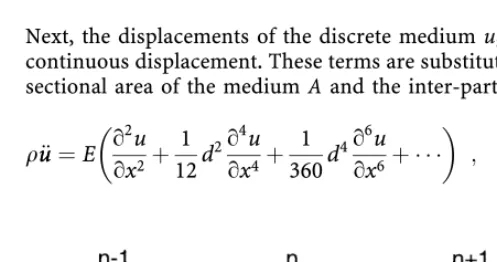
In this section, higher-order strain gradient models are derived by means of homogenisation of the displacement field of a discrete model. In the discrete model, the particles are represented by individual masses. The inter-particle contacts are modelled via springs that connect the masses. For simplicity, it is assumed that all particles have the same spring stiffnessK, particle massMand inter-particle distanced. This geometry is depicted in Fig. 2 for which the equation of motion of particle ncan be expressed as

Muun€ þKð2ununþ1un1Þ ¼0 ; ð13Þ

where a superimposed dot denotes a time derivative. In the homogenisation procedure, it is assumed that thecontinuousdisplacementuequals the discrete displacementunat particlen.

The displacement at the neighbouring particles is found by means of a Taylor series as

uðxdÞ ¼uðxÞ douðxÞ

ox þ 1 2d

2o2uðxÞ

ox2

1 6d

3o3uðxÞ

ox3 þ

1 24d

4o4uðxÞ

ox4 þ : ð14Þ

Next, the displacements of the discrete mediumunþ1andun1 are expressed in terms of the continuous displacement. These terms are substituted into Eq. (13). After division by the cross-sectional area of the medium Aand the inter-particle distancedit is found that

quu€¼E o

2

u ox2þ

1 12d

2o4u

ox4þ

1 360d

4o6u

ox6þ

; ð15Þ

Fig. 2. Discrete medium – geometri-cal and mechanigeometri-cal properties

with the mass density q¼M=Adand the Young’s modulusE¼Kd=A. Note that all odd derivatives ofu have cancelled.

When the kinematic relatione¼ou=oxis used, and the equation of motion of the con-tinuum is expressed asquu€¼or=ox, the constitutive relation can be retrieved as

r¼E eþ 1 12d

2o2e

ox2þ

1 360d

4o4e

ox4þ

: ð16Þ

When Eq. (16) is truncated after the second-gradient term, a constitutive relation with the format of Eq. (2) is found, i.e. the second-gradient term is preceded by a positivesign, where d¼lpffiffiffiffiffi12. Indeed, the above procedure illustrates the close relation between the discrete microstructure and the higher-order continuum according to Eq. (16).

As an alternative, it is possible to truncate Eq. (16) after the fourth-gradient term. Thus, a fourth-order strain-gradient model is obtained, [27, 28].

The homogenisation procedure as shown above unequivocally leads to a second-order strain-gradient term that is preceded by a positive sign, [10, 18, 28, 29]. Indeed, the second-gradient model with the negative sign, see Eq. (1), cannot be derived directly from a micro-structure of discrete particles.

4

Dispersion analysis

As a first exploration of the performance of the various models, an analysis of dispersive waves is carried out. Dispersive behaviour of a medium is characterised by its ability to change the shape of propagating waves. In a mathematical context, this implies that the wave velocity must depend on the wave number.

To investigate the dispersive character of the discrete model of Eq. (13), the harmonic solution

un ¼uu^expðikðctxnÞÞ

is substituted, in whichuu^is the amplitude,k is the wave number,cis the phase velocity,tis time andxnis the coordinate of particlen. The wave number is related to the wave lengthkvia kk¼2p. Using xn¼nd;xnþ1¼ ðnþ1Þd andxn1¼ ðn1Þd, it is found that

Mk2c2

K ¼4 sin

2 kd

2 : ð17Þ

The angular frequency xis defined asx¼ck and the elastic bar velocity isce¼ ffiffiffiffiffiffiffiffi E=q p

¼ ffiffiffiffiffiffiffiffiffiffiffiffiffiffiffi

Kd2_=M p

. Consequently, the dispersion relation of the discrete medium can be expressed as

x ce¼

2 d sin

kd 2

: ð18Þ

A similar procedure is followed for the continuum models. Starting point is the one-dimen-sional equation of motion quu€¼or=ox, in which the various constitutive equations and the kinematic relation are substituted. In the resulting expression on the harmonic solution u¼uu^expðikðctxÞÞis substituted. For the second-gradient model with the negative sign, see Eq. (1), this results in

x ce¼k

ffiffiffiffiffiffiffiffiffiffiffiffiffiffiffiffiffiffiffiffiffiffiffi 1þ 1

12k

2_d2

r

; ð19Þ

with d¼lpffiffiffiffiffi12. Since the second-order gradient model with a negative sign has not been derived from the discrete medium, the factor 1/12 is arbitrary. However, for a consistent comparison with the other models this factor has been adopted in the remainder of this study.

The dispersion relation for the second-gradient model with the positive sign (that is, the second-gradient truncation of Eq. (16)) reads

x ce¼k

ffiffiffiffiffiffiffiffiffiffiffiffiffiffiffiffiffiffiffiffiffiffiffi 1 1

12k

2_d2

r

; ð20Þ

and the dispersion relation for the fourth-gradient model taken from Eq. (16) can be elaborated as

x ce¼k

ffiffiffiffiffiffiffiffiffiffiffiffiffiffiffiffiffiffiffiffiffiffiffiffiffiffiffiffiffiffiffiffiffiffiffiffiffiffiffiffiffiffiffiffiffi 1 1

12k

2_d2_þ 1

360k

4_d4

r

: ð21Þ

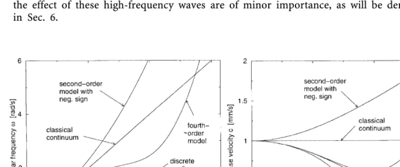
In Fig. 3, the dispersion curves for the various models are plotted, taking ce¼1 mm/s and

d¼1 mm. For comparison also the dispersion relation of the classical continuum is plotted. While the classical continuum is nondispersive (the phase velocityc¼x=kis constant), the discrete medium and the higher-order strain gradient continua are dispersive. It can be seen that the second-gradient model with the positive sign and the fourth-gradient model give improved approximations of the discrete model, as compared to the classical continuum. On the other hand, the agreement between the second-gradient model with the negative sign and the discrete medium is poor.

However, the instability of the second-gradient model with the positive sign also becomes manifest in Fig. 3: for wave numbers larger than pffiffiffiffiffi12=d the angular frequency and the phase velocity become imaginary, cf. Eq. (20). This means that waves with larger wave numbers (or, equivalently, with smaller wave lengths) cannot propagate through this medium. Instead, the imaginary frequency and velocity imply that the response occurs everywhere in the medium instantaneously. This is physically unrealistic. Therefore, these smaller wave lengths should not be considered. Filtering shorter waves occurs automatically in a discrete medium, where wave lengths smaller than two times the particle size cannot be monitored. However, in a continuous medium, all wave lengths can in principle be present. Especially when shock waves are investigated, all wave lengths are triggered by the loading. The imaginary angular frequency (or phase velocity) of these high-frequent waves prohibits a proper wave propagation simulation with this model, as will be illustrated in Sec. 6. The cut-off value for the wave number, i.e. the wave number for which the angular frequency is zero, dominates the static response of the second-gradient model with a positive sign. This cut-off value emerges at k¼pffiffiffiffiffi12=d, cf. Fig. 3.

It must be emphasized that for the second-gradient model with the negative sign, as well as for the fourth-gradient model, a range of wave numbers exists for which the phase velocity is larger than the bar velocity of the classical continuum, for which a physical motivation is lacking. For the second-gradient model with the negative sign, this covers the complete range of wave numbers, while for the fourth-gradient model it only concerns the higher wave numbers, see Fig. 3. However, in the response of the fourth-gradient model the effect of these high-frequency waves are of minor importance, as will be demonstrated in Sec. 6.

Fig. 3. Angular frequency versus wave number (left) and phase velocity versus wave number (right)

5

Linear static analysis

The higher-order gradient models are tested in a one-dimensional boundary value problem of which the geometry and the loading conditions are given in Fig. 4. An imperfection is placed in the centre of the bar to trigger order gradient activity. Due to the presence of higher-order terms in the governing equations, additional boundary conditions are required. Following the literature, we impose zero values for the first-order spatial derivative of the strain at the boundaries in the second-gradient model, [6, 19, 22, 25]. Moreover, zero values for the third-order spatial derivative of the strain are imposed at the boundaries in the fourth-gradient model, [6]. The bar of Fig. 4 is subjected to an imposed displacement of 0.01 mm at its right end which corresponds to an average strain level of 0.001. The Young’s modulus is taken as E¼1000 MPa.

Analytical solutions are available for the one-dimensional linear elastic case. However, in multi-dimensional cases numerical solution techniques are necessary. Therefore, the perfor-mance of the models is tested numerically. The problem has been solved by means of the element-free Galerkin (EFG) method, [8, 9]. This is a meshless discretisation method in which the shape functions can be formulated with an arbitrary order of continuity, which is advan-tageous when higher-order gradient models are investigated, [5, 6, 15, 20]. Discretisation aspects are treated in Appendix A. The bar of Fig. 4 has been discretised with 81 equally-spaced nodes and 400 equally-spaced integration points.

5.1

Second-gradient model with positive sign

The second-gradient model with the positive sign has been used, see Eq. (2), withd¼lpffiffiffiffiffi12. For this model, the solution has a harmonic character, see Eq. (4). The number of wave lengths along the bar isn¼L=k, withLdenoting the bar length andkthe wave length. The wave length is related to the wave numberkviak¼2p=k, while the critical wave number of the static case can be retrieved from the dispersion relation by requiring that the angular frequency (or the phase velocity) equals zero. This wave number equalsk¼pffiffiffiffiffi12=d, see Fig. 3. Thus, the number of wave lengths along the bar is given by

n¼L

ffiffiffiffiffi 12 p

2pd : ð22Þ

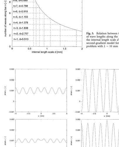
When this equation is compared to Eq. (9), and it is realised thatd¼lpffiffiffiffiffi12for the current model, it can be seen that uniqueness fails in the casenfrom Eq. (22) equals the integerm. In Fig. 5, relation (22) is plotted for the problem in Fig. 4 where L¼10 mm. In this figure, especially these values ofd are denoted for whichnequals the integermand, thus, for which uniqueness fails.

Remark 3. Note the difference between the wave numberkand the number of wave lengths along the barn. The wave numberkdenotes the number of wave lengths that fit into 2p, whilen denotes the number of wave lengths that fit into the bar lengthL. More generally,kis geometry-independent, while ndepends on the geometry under consideration.

Analyses have been carried out for values ofdwherenis an integer and for values ofdwhere nis not an integer. In Fig. 6, results of both types have been plotted; takingd¼0:8 mm or d¼0:7 mm leads to a noninteger value ofn, while takingd¼0:778 mm andd¼0:689 mm leads ton¼7 andn¼8, respectively. It can be verified that the number of wave lengths along the bar as given by the numerically obtained strain profiles corresponds perfectly to the value of nas given by Eq. (22) or Fig. 5. For the two analyses wherenis not an integer (Fig. 6, left

Fig. 4. Bar: problem statement for static analysis

column), uniqueness is guaranteed; as such, moderate oscillations in the strain profile are obtained. In contrast, whennis an integer (Fig. 6, right column) the solution is nonunique, which becomes manifest by the extreme oscillations in the strain profile. In fact, the analytical solution for the cases thatnis an integer is undetermined, causing the numerical solution to be arbitrarily dependent on round-off errors and discretisation aspects. In short, the static analysis shows that the results should be distrusted for a limited number of values for the internal length scaled. However, it remains an undesirable feature of this model that a local perturbation, as given by the imperfection in Fig. 4, leads to strain oscillations in the complete domain.

Fig. 6. Bar: static response of the second-gradient model with positive sign, strain profiles ford¼0:8 mm (top left),d¼0:788 mm (top right),d¼0:7 mm (bottom left) andd¼0:689 mm (bottom right)

Fig. 5. Relation between the number of wave lengths along the barnand the internal length scaledof the second-gradient model for the bar problem withL¼10 mm

5.2

Second-gradient model with negative sign

Next, the second-gradient model with the negative sign, Eq. (1), is used to analyse the problem of Fig. 4. As has been mentioned in Sec. 2, the analytical solution has an exponential character. No instabilities are to be expected, and uniqueness is guaranteed. Fig. 7 shows the response of this model for values of the internal length scaled¼0:5 mm andd¼1 mm. Although the cross-sectional area is discontinuous over the bar length, the strain profile along the bar is smooth due to the higher-order strain gradients that are present in the constitutive relation. This smoothing effect becomes more pronounced for larger values of the internal length scale d. Furthermore, local perturbations remain local. Thus, the second-gradient model with the negative sign yields physically realistic results.

5.3

Fourth-gradient model

Finally, the performance of the fourth-gradient model is tested for the bar problem of Fig. 4. A general analytical expression for the displacement field in the bar can be derived as (see Appendix B)

u¼C1þC2xþexp

s1x

d

C3cos

s2x

d

þC4sin

s2x

d

h i

þexp s1x d

C5cos

s2x

d

þC6sin

s2x

d

h i

;

ð23Þ

whereCi are constants that have to be determined according to the boundary conditions.

Furthermore, s1¼

ffiffiffiffiffiffiffiffiffiffiffiffiffiffiffiffiffiffiffiffiffiffiffiffi_{ffiffiffiffiffi} 90 p

15=2 q

ands2¼

ffiffiffiffiffiffiffiffiffiffiffiffiffiffiffiffiffiffiffiffiffiffiffiffi_{ffiffiffiffiffi} 90 p

þ15=2 q

are model-specific coefficients, which follow from the factors 1/12 and 1/360 that precede the second-gradient and fourth-gradient terms in the constitutive relation Eq. (16). From Eq. (23), it can be seen that the harmonic terms of the solution are multiplied with exponential terms. This implies that local perturbations of the strain field can remain local, which is in contrast to the response of the second-gradient model with the positive sign.

The coefficient of the harmonic terms in Eq. (23) equalss2=d. In the second-gradient model with the positive sign, the wave number has been found as k¼pffiffiffiffiffi12=din the argument of the harmonic terms of the analytical solutions. With these considerations, for the fourth-gradient model, the number of wave lengths along the bar can be found by replacing the factor pffiffiffiffiffi12in Eq. (22) by the factor s2. Thus,

n¼L

ffiffiffiffiffiffiffiffiffiffiffiffiffiffiffiffiffiffi_{ffiffiffiffiffi} 90 p

þ15 2

q

2pd : ð24Þ

Again,d can be selected such thatn equals an integer. However, in contrast to the second-gradient model, no anomalies are expected from the point of view of uniqueness, energy considerations or dispersion analysis when nis an integer.

Fig. 7. Bar: static response of the second-gradient model with negative sign, strain profiles for d¼0:5 mm (left) andd¼1 mm (right)

Four numerical analyses have been carried out, two with a value for the internal length scale dwherenis an integer, and two with a value fordwherenis not an integer. In Fig. 8, the strain profiles plotted for the casesd¼0:8 mm,d¼0:729 mm (which corresponds ton¼9),d¼0:7 mm andd¼0:656 mm (which corresponds ton¼10). The four results show very little differences. Indeed, instabilities are absent in the fourth-gradient model. Another important observation is that local perturbations of the strain field remain local and do not extend over the entire domain, which is physically realistic.

6

Linear dynamic analysis

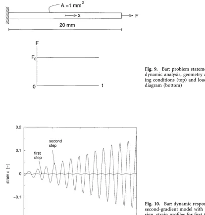
The problem statement for the dynamic analysis is given in Fig. 9. A Heaviside loading function is applied so that a shock wave propagates through the bar. The force amplitude isF0¼5 N, the Young’s modulus is taken asE¼1000 MPa, and the mass density isq¼1000 N s2=mm4_. For the spatial discretisation, the EFG method is used. Again, 81 equally-spaced nodes and 400 equally-spaced integration points have been used. For the time discretisation, the implicit Newmark scheme is used, [14, 25], with the time stepDt¼0:2 s and the Newmark parameters c¼0:5 andb¼0:25 (average acceleration method), unless mentioned otherwise. Although not shown here, similar results have been found for smaller time steps.

6.1

Second-gradient model with positive sign

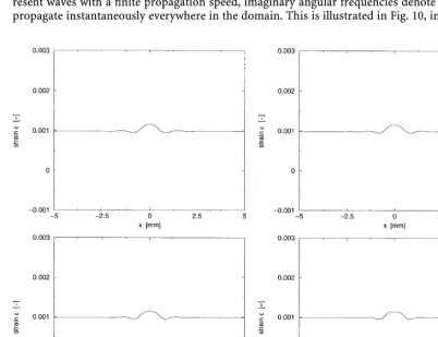
Firstly, the second-gradient model with the positive sign is taken to model the problem of Fig. 9. In the problem under consideration, in which a shock wave is generated, all harmonics are present in the response. As can be seen from Fig. 3, this implies that wave numbers with real frequencies (lower wave numbers) as well as wave numbers with imaginary frequencies (higher wave numbers) are triggered by the loading conditions. While real angular frequencies rep-resent waves with a finite propagation speed, imaginary angular frequencies denote waves that propagate instantaneously everywhere in the domain. This is illustrated in Fig. 10, in which the

Fig. 8. Bar: static response of the fourth-gradient model, strain profiles ford¼0:8 mm (top left), d¼0:729 mm (top right),d¼0:7 mm (bottom left) andd¼0:656 mm (bottom right)

dynamic response of the second-gradient model is plotted for the problem of Fig. 9. The internal length scale isd¼2 mm. Only the strain profiles corresponding to the first two time increments are plotted. It can be seen that after the first time increment the influence of the shock wave is present in the entire bar, which is unrealistic. After the second time increment, the amplitude of the strain profile increases in an unphysical manner to unrealistically large values. In the classical continuum, the strain profile would have propagated only marginally, while the amplitude would have remained bounded.

As such, the second-gradient model with a positive sign is unsuitable for numerical dynamic analyses. While the model instabilities in staticsare restricted to specific choices forn(Eq. (22)), the use of this model indynamics leads to anomalies for any loading condition that triggers wave numbers larger than the critical valuepffiffiffiffiffi12=d.

6.2

Second-gradient model with negative sign

Next, the second-gradient model with the negative sign has been used to simulate the problem of Fig. 9. As has been noted in Fig. 3, in this model no imaginary angular frequencies occur. However, all wave lengths are associated with phase velocities that are higher than that of the classical continuum.

Fig. 9. Bar: problem statement for dynamic analysis, geometry and load-ing conditions (top) and load-time diagram (bottom)

Fig. 10. Bar: dynamic response of the second-gradient model with positive sign, strain profiles for first two time steps

In Fig. 11, the strain profiles at time t¼4 s,t¼8 s,t¼12 s andt¼16 s are plotted. A range of values for the internal length scaledhas been taken, including the case of the classical continuum d¼0 mm. Ford>0, it can be seen that the shape of the front changes with increasing time, which illustrates the dispersive character of the medium. This dispersive effect is the result of the inclusion of higher-order gradients; in a classical continuum (the case with d¼0 mm in Fig. 11) the shape of the front remains unaltered in time (neglecting numerical dispersion effects). For larger values of d, the dispersion becomes more significant. Another observation is that, for finite values ofd, the front of the wave propagates faster than for the case d¼0, which is consistent with the dispersion analysis in Sec 4. This unrealistically fast propagation speed of the wave front is a disadvantage of this model.

6.3

Fourth-gradient model

Finally, the fourth-gradient model is used for modelling the problem in Fig. 9. In contrast to the second-gradient model with a positive sign, no wave numbers with imaginary angular fre-quencies exist, as can be verified from Fig. 3. Thus, the numerical deficiencies as they have appeared for the second-gradient model with a positive sign are not to be expected for the fourth-gradient model.

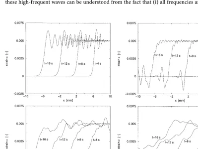
In Fig. 12, the propagation of the strain profile is plotted for a range of internal length scales d, and at timet¼4 s, t¼8 s,t¼12 s andt¼16 s. In comparison with the response of the second-gradient model with the positive sign, in the fourth-gradient model the strain profile propagates in a realistic manner for all values of d. The propagation speed is finite, and the amplitude of the strain profile remains bounded. It can be seen that, depending on the value of d, the front of the wave changes in shape during the propagation. For higher values ofd, the dispersive character of the model becomes more pronounced.

A peculiar phenomenon that occurs in all analyses with d>0 is the appearance of high-frequent waves that propagate ahead ofthe actual front of the strain profile. The existence of these high-frequent waves can be understood from the fact that (i) all frequencies are triggered

Fig. 11. Bar: dynamic response of the second-gradient model with negative sign, propagation of the strain profile ford¼0 mm (top left),d¼0:5 mm (top right),d¼2 mm (bottom left) andd¼5 mm (bottom right)

by the current shock-wave loading conditions, and (ii) in the present fourth-gradient model, the higher wave numbers are associated with phase velocities that are larger than the bar velocitypffiffiffiffiffiffiffiffiE=q(see Fig. 3). In contrast, in the response of the second-gradient model with the negative sign,allwave numbers have a phase velocity larger than the bar velocity, causing the propagation speed of the complete wave front to be unrealistically high.

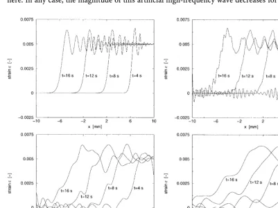
Damping of the artificial high-frequency fast-propagating waves can be attained in various ways. For instance, the Newmark parameter ccan be increased, [14, 26]. In Fig. 13, the propagating strain profile is plotted again for the case d¼2 mm, but now withc¼0:7 and b¼ ðcþ1=2Þ2=4¼0:36. Indeed, numerical damping of the high frequencies is obtained, although a high-frequency wave propagating faster than the wave front still appears. Alter-natively, the combination of an implicit time integration scheme with a lumped mass matrix may be considered to increase numerical damping, [26], although this option is not considered here. In any case, the magnitude of this artificial high-frequency wave decreases for increasing

Fig. 12. Bar: dynamic response of the fourth-gradient model, propagation of the strain profile for d¼0 mm (top left),d¼0:5 mm (top right),d¼2 mm (bottom left) andd¼5 mm (bottom right)

Fig. 13. Bar: dynamic response of the fourth-gradient model withd¼2 mm; influence of Newmark parameters:c¼0:5 andb¼0:25 (left),c¼0:7 andb¼0:36 (right)

time, so that eventually its influence will become negligible. Furthermore, it must be realised that the discretisation sets an upper bound to the wave numbers that can be transmitted; the infinitely high wave numbers that would travel with an infinitely high velocity can never be captured by a finite discretisation fineness.

7

Conclusions

In this paper, several types of strain-gradient models are studied. A distinction is made between two motivations for the incorporation of higher-order strain gradients into a classical continuum: firstly, regularisation or smoothing of singularities or discontinuities in the strain field, and, secondly, the introduction of heterogeneity. In both cases, an internal length scale related to the size of the microstructure enters the model. A typical second-order strain-gradient model of either case is studied analytically, where it has been found that the sign of the second-order gradient term drives the uniqueness and the stability of the model. A second-gradient model with a negative sign, as is classically used to regularise singularities, guarantees uniqueness and stability, but lacks a direct link with the underlying microstructure. On the other hand, a second-gradient model with positive sign can be derived directly from a discrete medium, but the model can become unstable and uniqueness is not guaranteed.

To combine the advantageous properties of the two types of second-gradient models, a fourth-order strain-gradient model is derived from a discrete medium. It is demonstrated that this fourth-gradient model is unconditionally stable, while the link with the underlying microstructure is evident.

Linear static and dynamic numerical analyses have been carried out to assess the perfor-mance of the higher-order gradient models. The element-free Galerkin method has been used, since this method facilitates the incorporation of higher-order strain gradients.

The static response of the second-gradient model with a positive sign is found to be unstable for a selected number of values of the internal length scale. In other cases, a stable response is found, although local perturbations lead to oscillations in the entire domain. The responses of the second-gradient model with a negative sign and of the fourth-gradient model in statics are physically realistic and mathematically sound: no instabilities are found, and local perturba-tions remain local.

In dynamics, the differences between the models become more pronounced. The second-gradient model with positive sign fails completely due to imaginary propagation velocities of the higher wave numbers. These higher wave numbers are especially dominant when shock waves are generated. Thus, this second-gradient model is not suitable to study practical dy-namic problems. The second-gradient model with negative sign gives stable results, but all waves propagate with a velocity that is unrealistically high (i.e. higher than the bar velocity of the classical continuum). On the other hand, in the fourth-gradient model, all propagation velocities are real, and realistic responses are found. The model shows a dispersive character, and the intensity of the dispersion depends on the internal length scale parameter. However, waves are found that propagate with an unrealistically high velocity, but this only concerns the higher wave numbers, and their influence on the global response appears to be limited in the presented analysis.

Appendix A

Discretisation aspects

Below, the discretised system of equations will be derived that has been used to perform the EFG analysis with the higher-order gradient continua in Secs. 5 and 6. Starting point is the weak format of the one-dimensional equation of the motion, i.e.

ZL

0

duq€uudx¼ ZL

0

duor

oxdx ; ð25Þ

in which body forces are left out of consideration. The general constitutive equation is written as

r¼Eðeþc1r2eþc2r4eÞ ; ð26Þ

where ðc1;c2Þ ¼ ð1 12d

2_{;0Þfor the second-gradient model with a positive sign,} ðc1;c2Þ ¼ ð1

12d

2_{;0Þ for the second-gradient model with negative sign, and} ðc1;c2Þ ¼ ð1

12d 2_; 1

360d

4_{Þfor the fourth-gradient model. Equation (26) is substituted into Eq. (25),} the kinematic relation e¼ou=oxis used, and the higher-order terms are integrated by parts. Thus,

ZL

0

duq€uudxþ

Z L

0

odu ox E

ou oxdx

ZL

0

o2du ox2 Ec1

o2u ox2dx

þ ZL

0

o3du ox3 Ec2

o3u

ox3dx¼ duEðeþc1r 2_eþc

2r4eÞ

L

0

odu ox Ec2

o4u ox4

L

0

: ð27Þ

The first boundary term in the right-hand-side of Eq. (27) can be identified as the conventional traction boundary term. The second boundary term cancels by assuming vanishing fourth-order derivatives of the displacement, [6]. The first two domain integrals in the left-hand-side of Eq. (27) concern with the conventional mass matrix and stiffness matrix, respectively. The third and fourth domain integral represent the higher-order contributions of the models. After discretisation, a global system of equations is obtained as

M€uuþ ½K0þK1þK2u¼f ; ð28Þ

whereu contains the discretised displacements. Furthermore,

M¼

ZL

0

q/_u/T_udx ; ð29Þ

K0 ¼

ZL

0

Eo/u ox

o/T_u

ox dx ; ð30Þ

K1 ¼

ZL

0

Ec1

o2/_u ox2

o2/T_u

ox2 dx ; ð31Þ

K2 ¼

ZL

0

Ec2

o3/_u ox3

o3/T_u

ox3 dx ; ð32Þ

f ¼ ½/_u^_tt

Cn ; ð33Þ

where^_{tt are the prescribed tractions on the boundary}Cn.

Remark 4. Each subsequent derivative of an EFG shape function has a more oscillatory character than the previous one. To avoid zero-energy modes, the order of integration should be increased in correspondence with thehighestderivative of the shape functions that appears in the formulation.

Appendix B

Displacement field of fourth-order model

To determine the displacement field of the fourth-order model, a general expression for the displacement u¼expðikxÞis substituted in the homogeneous equilibrium equation

o2uðxÞ ox2 þ

1 12d

2o 2_uðxÞ

ox4 þ

1 360d

4o 6_uðxÞ

ox6 ¼0 : ð34Þ

This leads to

k2 ¼0 _ 1

360ðdkÞ

4 1

12ðdkÞ

2_þ

1¼0 : ð35Þ

The case k2 _{¼0 leads to the displacement field of the classical continuum. The higher-order} contribution is given through four values for dkas

dk¼

ffiffiffiffiffiffiffiffiffiffiffiffiffiffiffiffiffiffiffiffiffiffiffi 15i3pffiffiffiffiffi15 q

: ð36Þ

The square root of a general complex number aþibis rewritten via

ffiffiffiffiffiffiffiffiffiffiffiffiffi aþib p

¼p4ffiffiffiffiffiffiffiffiffiffiffiffiffiffiffia2_þb2

exp i arctanðb=aÞ 2

: ð37Þ

Furthermore, the following goniometric relations are used.

cos arctanðb=aÞ 2

¼

ffiffiffiffiffiffiffiffiffiffiffiffiffiffiffiffiffiffiffiffiffiffiffiffiffiffiffiffiffiffiffiffiffiffiffiffiffiffiffiffiffiffi 1þcosðarctanðb=aÞÞ

2 r ¼ ffiffiffiffiffiffiffiffiffiffiffiffiffiffiffiffiffiffiffiffiffiffiffiffiffiffiffiffiffi 1 2þ a 2pffiffiffiffiffiffiffiffiffiffiffiffiffiffiffia2_þb2

s ; ð38Þ sin arctanðb=aÞ 2 ¼ ffiffiffiffiffiffiffiffiffiffiffiffiffiffiffiffiffiffiffiffiffiffiffiffiffiffiffiffiffiffiffiffiffiffiffiffiffiffiffiffiffiffi 1cosðarctanðb=aÞÞ

2 r ¼ ffiffiffiffiffiffiffiffiffiffiffiffiffiffiffiffiffiffiffiffiffiffiffiffiffiffiffiffiffi 1 2 a 2pffiffiffiffiffiffiffiffiffiffiffiffiffiffiffia2_þb2

s

; ð39Þ

With these substitutions, Eq. (36) is rewritten as

dk¼ i

ffiffiffiffiffiffiffiffiffiffiffiffiffiffiffiffiffiffiffiffiffiffiffiffi_{ffiffiffiffiffi} 90

p

15=2 q

ffiffiffiffiffiffiffiffiffiffiffiffiffiffiffiffiffiffiffiffiffiffiffiffi_{ffiffiffiffiffi} 90

p

þ15=2 q

: ð40Þ

Introducing s1¼

ffiffiffiffiffiffiffiffiffiffiffiffiffiffiffiffiffiffiffiffiffiffiffiffi_{ffiffiffiffiffi} 90 p

15=2 q

ands2¼

ffiffiffiffiffiffiffiffiffiffiffiffiffiffiffiffiffiffiffiffiffiffiffiffi_{ffiffiffiffiffi} 90 p

þ15=2 q

, and eliminating the imaginary parts of the solution, the total homogeneous solution of Eq. (34) is found as

u¼C1þC2xþexp

s1x

d

C3cos

s2x

d

þC4sin

s2x

d

h i

þexp s1x d

C5cos

s2x

d

þC6sin

s2x

d

h i

: ð41Þ

References

1. Aifantis, E.C.:The physics of plastic deformation. Int J Plasticity 3 (1987) 211–247

2. Aifantis, E.C.:Gradient deformation models at nano, micro, and macro scales. ASME J Eng Mat Tech 121 (1999) 189–202

3. Aifantis, E.C.:Strain gradient interpretation of size effect. Int J Fracture 95 (1999) 299–314

4. Altan, B.S.; Aifantis E.C.:On some aspects in the special theory of gradient elasticity. J Mech Behavior Mat 8 (1997) 231–282

5. Askes, H.:Advanced spatial discretisation strategies for localised failure – mesh adaptivity and meshless methods. Dissertation, Delft University of Technology, 2000

6. Askes, H.; Pamin, J.; de Borst, R.:Dispersion analysis and element-free Galerkin solutions of second and fourth-order gradient-enhanced damage models. Int J Numer Methods Eng 49 (2000) 811–832

7. Askes, H.; Suiker, A.S.J.; Sluys, L.J.:Dispersion analysis and element-free Galerkin simulations of higher-order strain gradient models. Mat Phys Mech 3 (2001) 12–20. Also available at http:// www.ipme.ru

8. Belytschko, T.; Krongauz, Y.; Organ, D.; Fleming, M.; Krysl, P.:Meshless methods: an overiew and recent developments. Computer Meth Appl Mech Eng 139 (1996) 3–47

9. Belytschko, T.; Lu, Y. Y.; Gu, L.:Element-free Galerkin methods. Int J Numer Meth Eng 37 (1994) 229–256

10. Chang, C.S.; Gao, J.:Second-gradient constitutive theory for granular material with random packing structure. Int J Solids Struct 32 (1995) 2279–2293

11. Comi, C.; Driemeier, L.:On gradient regularization for numerical analysis in the presence of damage. In: de Borst R., van der Giessen E. (eds) Material Instabilities in Solids, Chap. 26, pp. 425–440. Amsterdam: Wiley 1998

12. de Borst, R.; Mu¨hlhaus, H.-B.:Gradient-dependent plasticity: formulation and algorithmic aspects. Int J Numer Meth Eng 35 (1992) 521–539

13. Geers, M.G.D.:Experimental analysis and computational modelling of damage and fracture. Disser-tation, Eindhoven University of Technology, 1997

14. Hughes, T.J.R.:The Finite Element Method – Linear Static and Dynamic Finite Element Analysis. London: Prentice-Hall 1987

15. Jira´sek, M.:Element-free Galerkin method applied to strain-softening materials. In: de Borst R., Bic´anic´ N., Mang H., Meschke G. (eds) Computational Modelling of Concrete Structures, pp. 311–319. Rotterdam: Balkema 1998

16. Lasry, D.; Belytschko, T.:Localization limiters in transient problems. Int J Solids Struct 24 (1988) 581–597

17. Mu¨hlhaus, H.-B.; Aifantis, E.C.:A variational principle for gradient plasticity. Int J Solids Struct 28 (1991) 845–857

18. Mu¨hlhaus, H.-B.; Oka, F.:Dispersion and wave propagation in discrete and continuous models for granular materials. Int J Solids Struct 33 (1996) 2841–2858

19. Pamin, J.:Gradient-dependent plasticity in numerical simulation of localization phenomena. Disser-tation, Delft University of Technology, 1994

20. Pamin, J.; Askes, H.; de Borst, R.:An element-free Galerkin method for gradient plasticity.

In: Wunderlich W. (ed) European Conference on Computational Mechanics – Solids, Structures and Coupled Problems in Engineering, TU Mu¨nchen, 1999

21. Peerlings, R.H.J.:Enhanced damage modelling for fracture and fatigue. Dissertation, Eindhoven University of Technology, 1999

22. Peerlings, R.H.J.; de Borst, R.; Brekelmans, W.A.M.; de Vree, J.H.P.:Gradient enhanced damage for quasi-brittle materials. Int J Numerical Meth Eng 39 (1996) 3391–3403

23. Peerlings, R.H.J.; de Borst, R.; Brekelmans, W.A.M.; de Vree, J.H.P.; Spee, I.:Some observations on localisation in non-local and gradient damage models. Eur J Mech A/Solids 15 (1996) 937–953

24. Schreyer, H.L.; Chen, Z.:One-dimensional softening with localization. ASME J Appl Mech 53 (1986) 791–797

25. Sluys, L.J.:Wave propagation, localisation and dispersion in softening solids. Dissertation, Delft University of Technology, 1992

26. Sluys, L.J.; Cauvern, M.; de Borst, R.:Discretization influence in strain-softening problems. Eng Comput 12 (1995) 209–228

27. Suiker, A.S.J.; Askes, H.; Sluys, L.J.:Micro-mechanically based 1-D gradient damage models. In: On˜ate E., Bugeda G., Sua´rez B. (eds) European Congress on Computational Methods in Applied Sciences and Engineering, Barcelona: CIMNE, 2000

28. Suiker, A.S.J.; de Borst, R.; Chang, C.S.:Micro-mechanically based higher-order continuum models for granular materials. In: Kolymbas D. (ed) Constitutive Modelling of Granular Materials, pp. 249–274. Heidelberg: Springer-Verlag, 2000

29. Suiker, A.S.J.; de Borst, R.; Chang, C.S.:Micro-mechanical modelling of granular material. Part 1: derivation of a second-gradient micro-polar constitutive theory. Acta Mech 149 (2001) 161–180

30. Suiker, A.S.J.; de Borst, R.; Chang, C.S.:Micro-mechanical modelling of granular material. Part 2: plane wave propagation in infinite media. Acta Mech 149 (2001) 181–200

31. Triantafyllidis, N.; Aifantis, E.C.:A gradient approach to localization of deformation. I. Hyperelastic materials. J Elas 16 (1986) 225–237

32. Triantafyllidis, N.; Bardenhagen, S.:On higher gradient continuum theories in 1-D non-linear elas-ticity. Derivation from and comparison to corresponding discrete models. J Elas 33 (1993) 259–293

33. Vardoulakis, I.; Exadaktylos, G.; Aifantis, E.C.:Gradient elasticity with surface energy: mode-III crack problem. Int J Solids Struct 33 (1996) 4531–4559