Testing coupled rotor blade-lag damper vibration dynamics using real-time dynamic substructuring

This is a repository copy of Testing coupled rotor blade-lag damper vibration dynamics using real-time dynamic substructuring.

White Rose Research Online URL for this paper: http://eprints.whiterose.ac.uk/79698/

Version: Accepted Version

Article:

Wallace, M.I., Wagg, D.J., Neild, S.A. et al. (3 more authors) (2007) Testing coupled rotor blade-lag damper vibration dynamics using real-time dynamic substructuring. Journal of Sound and Vibration, 307 (3-5). 737 - 754. ISSN 0022-460X

https://doi.org/10.1016/j.jsv.2007.07.004

Reuse

Unless indicated otherwise, fulltext items are protected by copyright with all rights reserved. The copyright exception in section 29 of the Copyright, Designs and Patents Act 1988 allows the making of a single copy solely for the purpose of non-commercial research or private study within the limits of fair dealing. The publisher or other rights-holder may allow further reproduction and re-use of this version - refer to the White Rose Research Online record for this item. Where records identify the publisher as the copyright holder, users can verify any specific terms of use on the publisher’s website.

Takedown

If you consider content in White Rose Research Online to be in breach of UK law, please notify us by

Testing coupled rotor blade–lag damper

vibration dynamics using real-time dynamic

substructuring

M.I. Wallace

∗

, D.J. Wagg

, S.A. Neild

, P. Bunniss

,

N.A.J. Lieven

and A.J. Crewe

a_{Faculty of Engineering, University of Bristol, Queens Building, University Walk,}

Bristol BS8 1TR, U.K.

Citation:

Journal of Sound and Vibration:

307

:737–754, 2007.

Abstract

In this paper we present new results from laboratory tests of a helicopter rotor blade coupled with a lag damper from the EH101 helicopter. Previous modelling of this combined system has been purely numerical. However, this has proved challenging due to the nonlinear behaviour of the dampers involved — the fluid filled lag damper is known to have approximate piecewise linear force-velocity characteristics, due to blow-off valves which are triggered at a certain force level, combined with a strongly hysteretic dynamic profile. The novelty of the results presented here, is that the use of a hybrid numerical-experimental testing technique called real-time

such that there is bi-directional coupling between the numerical blade model and the experimental lag damper. The new results obtained from these tests (for steady state flight conditions) reveal how the inclusion of a real damper produces a more realistic representation of the dynamic characteristics of the overall blade system (during operational flight conditions) than numerical modelling alone.

Key words: Helicopter, lag-damper, real-time, substructuring, delay compensation.

1 Introduction

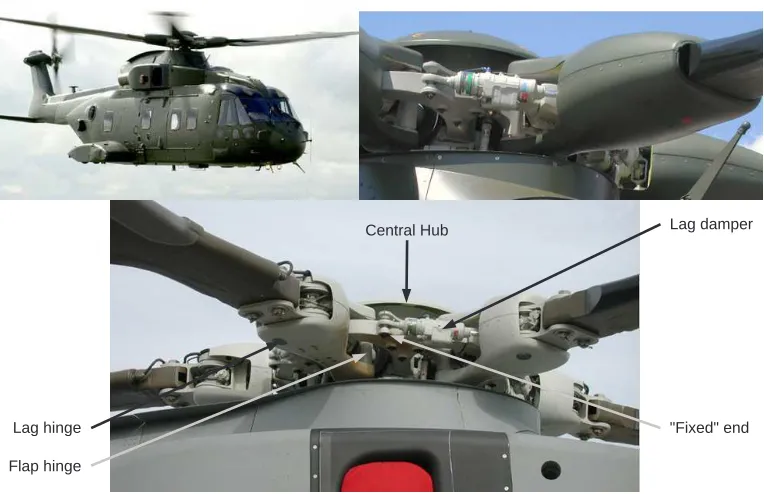
In this paper we present new results from laboratory tests of a lag damper for the EH101 helicopter (manufactured by Westland helicopters). Lag dampers are found on all fully-articulated helicopters, usually connected from the main rotor hub to the inboard section of each individual blade. They perform a vital function with respect to the stability of the aircraft by controlling blade motion and damping resonances — particularly at rotor start up, where the rotor frequency typically passes through a resonant region of the fuselage sys-tem (known as “ground resonance”) before reaching its operational frequency level. However, as a component of the rotor hub dynamic system, the damper influences the general vibration characteristics of the entire aircraft by gen-erating higher harmonic loads. This in tern forces the blade to respond at frequencies which are important when considering blade vibration.

The fluid filled lag-dampers have highly nonlinear dynamic characteristics and

∗

Corresponding author.

the effect of this nonlinear behaviour on the combined rotor blade–lag damper system is of significant interest in the design and manufacture of helicopters [1–4]. Previous modelling of this combined system has been purely numeri-cal which has proved challenging [5]. Initially, these models were linearized or simplified models of the damper’s dominant characteristic behaviour. More recently, Eyres [6] has developed a parametric model of the damper, based on an assumed piecewise linear force-velocity profile. Simulations carried out using this model when excited by recorded flight data have enabled designers to improve the modelling of the nonlinear behaviour present in the blade–lag damper system. However, without experimental validation, design confidence in any numerical model will remain low. The work presented in this paper, which builds on [6], shows results from hybrid numerical-experimental lab-oratory tests using a flight certified EH101 lag damper coupled to an eight mode modal model of a rotor blade excited by the same flight test data for steady-state trim flight conditions.

instantaneously to a change of state as prescribed by the numerical model. In some situations the transfer system delay may be so small as to be negligible, but the typical situation in substructuring is that this delay is large enough to have a significant influence on the overall dynamics of the substructured system. This error manifests itself as a form of negative damping, destabiliz-ing the hybrid system when the overall dampdestabiliz-ing becomes negative. However, using specific control techniques it is possible to cancel, or at least minimise, these unwanted dynamics to achieve a stable and accurate testing scheme.

Real-time dynamic substructuring allows design engineers to view the be-haviour of critical components — such as the lag damper — under dynamic loading in relation to the entire system, rather than in isolation, when it is impractical (or impossible) to house the complete system in a laboratory. So far the technique has been developed successfully using delayed time scales — known as pseudo-dynamic testing, for large civil engineering systems [9–

2 The EH101 lag damper

Hydraulic lag dampers create a force proportional to the square of the lag velocity by forcing fluid through an orifice. The damper studied here is a flight specification lag damper from an Agusta-Westland EH101 helicopter. This is a medium-lift helicopter originally developed as a joint venture between Westland Helicopters in the UK and Agusta in Italy for military applications but also marketed for civil use1_{. Figure 1 shows the EH101 helicopter and}

detailed views of the lag damper in position between the helicopter rotor hub and rotor blade.

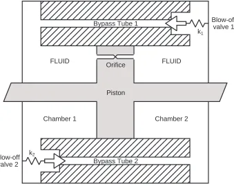
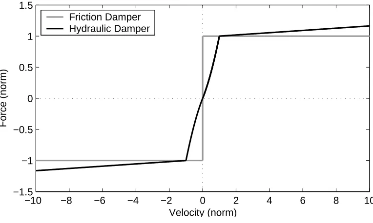
The main body of the damper consists of a cylindrical sealed chamber with a piston and rod passing through it — shown schematically in Figure 2. The damping force is generated as fluid is forced through the piston orifice. This mechanism generates high damping force values for relatively low velocities. In order to produce a useful force-velocity characteristic hydraulic dampers also require relief (or blow-off) valves to keep the damper loads to an acceptable level — a schematic diagram of a typical force-velocity profiles of an idealized hydraulic damper is shown in Figure 3. The EH101 lag damper makes use of two valves connected to the damper casing which are operated by linear springs, one for each direction of motion of the piston.

The force generated by the damper will act on the blade in the opposite sense

1 _{In 2001 Agusta-Westland signed a deal with Lockheed Martin to market the}

to the relative blade motion, damping the vibration of the blade in its lag degree of freedom (parallel to the ground). The damper is attached to the blade and hub using spherical bearings so that the damper force is assumed to act purely along the central axis of the damper piston.

2.1 Mathematical model of a coupled rotor blade–lag damper system

The model presented in this section is based on the derivation described by Eyres [6, 24], which in turn is based on much earlier work by NASA in the 1950’s and 60’s [25,26]. This derivation assumes the blades are forced period-ically by a constant matrix, representing steady-state trim forward flight. The analysis for a single blade uses 8 modes represented by modal displacements

φi where i= 1. . .8. The modes correspond to 4 flap modes, 3 lag modes and one twist mode. This low order modal model allows us to compute the blade response with minimal computational effort. The forcing effect of the damper is included on the right hand side of the forced response equation, thus giving the equation of motion for each mode to be

1 Ω2

d2φi dt2 +

2υB i λBi

Ω

dφi dt + (λ

B i )

2_{φi =} 1

IB i

(RF_icode+LDFiexp), i= 1. . .8 (1)

where λB

i is modal frequency, IiB modal inertia and υiB modal damping of a

blade with an angular velocity of Ω. The 8 modal equations are forced by the terms RFcode

i , which represents the modal forcing from the main rotor and LDFiexp which is the experimentally measured lag damper force transformed

to represent the effect of the lag damper force on each mode. We note that the modal forcing matrices are periodic functions of time (or azimuth). This effec-tive total modal forcing, which is part numerically defined (RFcode

i ) and part

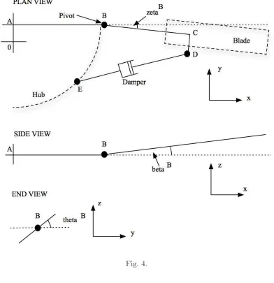
given by equation 1. The motion of the damper is defined by the coordinates in Figure 4.

The motion of the blade in the flap, lag and twist modes can be combined to produce the full motion of the blade relative to its fixed rotating position. The flap and lag angle of the blade are denoted by βB _{and ζ}B _{respectively. The}

flap and lag angles are calculated using the constant vectors ωDB (the modal

flap deflection) and ¯υDB (the modal lag deflection) which are multiplied by the

current modal state φ such that

βB =ω₀B_D +

8

X

i=1

φiωiB_D, (2)

ζB =υ₀B_D+

8

X

i=1

φiυ¯_iB_D, (3)

where,ωB

0D andυ

B

0D are the initial values. The angle of twist, θ

B_{, is defined as}

θB =θB₀ +dθ

B

0

dψ −A B

1cos(ψ)−B1Bsin(ψ), (4)

where, AB

1 and B1B are the lateral and longitudinal cyclic control angle

con-stants respectively, θB

0 is the initial angle and ψ is the azimuth angle. The

angular velocities in flap, lag and twist are defined as

dβB dψ = 8 X i=1 dφi dψω B

iD, (5)

dζB dψ = 8 X i=1 dφi dψυ¯

B

iD, (6)

dθB dψ =A

B

1sin(ψ)−B1Bcos(ψ). (7)

Using Figure 4 the rotation matrices can be derived as follows. The global position at points B and D (see Figure 4) is given by the vectors b _and d

twist as

d₌b_+TβTζTθ(d−b_{), (8)}

˙

d_{= ˙TβTζ}˙ _Tθ˙ ₍d−b_{), (9)}

where the rotation matrices for flap Tβ, lag Tζ and twist Tθ are given in the Appendix. The component of the velocities acting at point D along the damper axis then give the velocity of the damper piston, Vd, such that

Vd=T−1

γ Tδ−1d,˙ (10)

where Tγ and Tδ (given in the Appendix), relate to the angles γB and δB

representing the angles of the damper relative to the points D and the fixed point E on the hub. The angles are calculated from the relationships

δB= tan−1 "

d

Z−eZ

d

X−eX

#

, (11)

γB = cos−1



 "

(dX−eX

LD )

2_{+ (}dZ−eZ

LD )

2

#1

2



, (12)

where LD is the absolute distance between the two attachment points of the lag damper which is given by

LD = [(d

X −eX)2+ (dY −eY)2 + (dZ−eZ)2]

1

2. (13)

The resulting velocity, Vd, is taken as the output from the substructuring numerical model.

The force measured from the damper,F _{= [A∆P,0,0] (where, A is the}

cross-sectional area of the piston and ∆P is the pressure difference between cham-bers 1 and 2), is transformed back into the global axis system at D to give

F D _{so the modified forcing of the modes can be calculated as}

and at C using the fact that F C ₌F D_{:= [F CX, F CY, F CZ].}

The modal forcing provided by the damper is given for the ith _{mode as}

LDF_iexp= 1 Ω2

7

X

j=1

T_i(j), (15)

where the seven quantities T_i(j) are calculated for each mode using small angle approximations and constant vectors ωi_D, ¯υi_D and ti_D for flap, lag and twist — these are given in the Appendix.

2.2 Experimental testing set-up

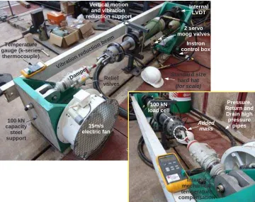
The experimental test rig itself is quite simple. Two 100kN steel supports are bolted directly into a steel T-slot in the “strong” floor of the laboratory with the central axis of the actuator and damper aligned. The base of the actuator is rigidly bolted into one support and then supported by a vertical stand. This stand has a height adjustment feature allowing for alignment and additionally ensures that the actuator does not vibrate during testing. A ±_{100kN Instron}

Dynacell dynamic load cell is then rigidly attached to the actuator piston. A yoke is required to connect the damper to the active part of the load cell. The extra mass of the yoke then acts as if it were part of the experimen-tal substructure component (the lag damper) which can distort the inertial response [27]. In this case the load cell force reading would be altered such that Fcell = Fdamper +myokeapiston. The yoke can be seen in Figure 5 and is labeled as added mass. The Instron Dynacell is a load measurement device which automatically compensates for load errors induced through inertia by automatically tuning a compensation factor klc which is used in conjunction with an internal axially mounted accelerometer alc. Thus,

Fcell =Fdamper+myokeapiston−_{klcalc =Fdamper. (16)}

In this situation dynamic inertia compensation is essential to maintain a high level of accuracy during real-time dynamic substructure testing.

gener-ated as heat. The damper is designed to operate at between ambient and 50o_C

in normal flight conditions, increasing to 80o_{C in desert conditions. The oil}

seals fail at 120o_{C. To keep the viscosity constant within the damper during}

operation (i.e. during changes in temperature) an internal mechanical spring-loaded compensator is integral to the damper’s design. In order to observe the temperature change during testing a K-series thermocouple has been attached to the outer casing of the damper and is read on a digital multi-meter — this is not used for any control, just to ensure the correct testing environment.

The base end of the lag damper is then bolted into a yoke directly attached to the remaining steel support. Finally, a 5 inch steel channel section is bolted directly onto the steel supports under tension. This preloads the rig which helps to remove any vibration and unwanted axial displacement. Under test conditions the unwanted axial displacement was measured at ±_{0.1mm over}

the entire length of the rig setup. Final fine scale alignment for the entire rig was carried out using a theodolite and a laser projection system.

The control of the test rig is achieved in a similar manner to that described in [19], with appropriate modifications to achieve the desired performance requirements. The control system consists of four constituent components:

(1) Control Hardware to drive the hydraulic actuator: Two state of the art Instron 8800 digital servo-hydraulic controllers are used to drive the hy-draulic actuator.

(2) Inner-loop PID controller: A standalone PC is used for the inner-loop

8800 controllers through dedicated software.

(3) Outer-loop substructuring controller: A second standalone PC is used for the substructuring algorithm and outer-loop control. The substructuring algorithm is designed in MATLAB/Simulink before being compiled and then built into the hard real-time processor of the dSpace DSP (see be-low). From this computer parameters in the substructuring algorithm can be controlled depending on the test being performed.

(4) dSpace DSP: The dSpace DS1103 R&D Controller Board is used to im-plement the substructuring algorithm experimentally in real-time. The substructuring algorithm is built into the processor (which operates at a clock speed of 500 MHz) and is connected to the Instron controller via an expansion board. The relevant signals are then passed between the Instron controller and the dSpace DSP under hard real-time constraints. The dSpace board outputs to the outer-loop PC in soft real-time for visualization.

2.3 Lag damper system identification

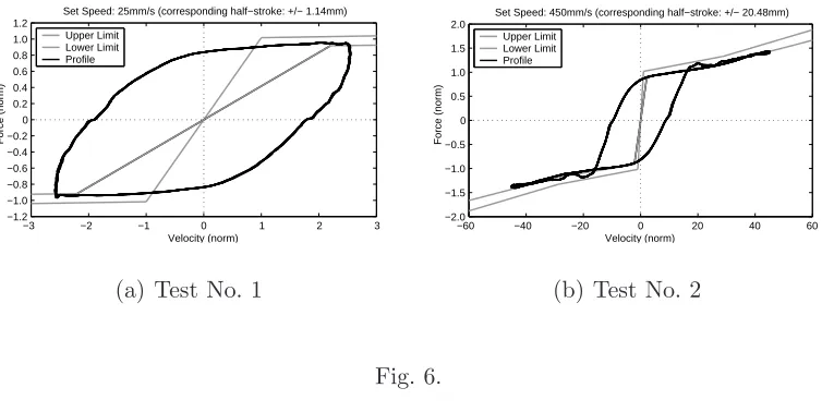
To initially characterise the nonlinearities in the damper a series of system identification tests were carried out. Results from two tests are presented and in both cases the input to the damper is sinusoidal at a frequency of 3.5Hz (that of the rotor system in flight). In test 1 the set speed was 25mm/s and the corresponding half-stroke ± _{1.14mm (just before the critical relief valve}

value is reached). In test 2 the set speed was 450mm/s and the corresponding half-stroke± _{20.46mm (full speed).}

The results from the two tests are shown in Figure 6 — these are experimen-tal force-velocity profiles produced by the damper for the differing set speed conditions for 5 seconds of steady state data. The experimental data is su-perimposed over the manufacture’s upper and lower tolerances. It should be noted that the entire profile is not designed to fit within these tolerances, in-stead just the peak positions. This highlights one of the major challenges in the understanding of the damper’s dynamic characteristics as when designing the damper, it is just these tolerance lines which are specified.

while the damper is being driven at high acceleration, sizeable nonlinear oscil-lations can be observed. The shape and magnitude of this nonlinearity was only found to be repeatable for each steady state test. Therefore, when the damper is not being driven in this simple manner, such as in-flight, it becomes increas-ingly complicated to model these nonlinear phenomena. The combination of these two nonlinearities, and the fact that they vary with the operational en-vironment of the damper, have made numerical modelling of such dampers extremely difficult. Additionally, we note that the slight nonlinearity at zero force is the actuator dead zone (a certain pressure is required to overcome the static friction of the piston) which will contribute to the experimental errors.

3 Experimental real-time substructure testing of the EH101 lag

damper

In these experimental tests we will consider the case of steady state flight at 84knots. We use this general flight case, along with a number of specific helicopter properties to define the constants for equation 1 which then set our steady state flight conditions — the details of this information are industrially sensitive and therefore cannot be published. In addition, the figures presented in this section have been normalized for the same reason.

3.1 Robust transfer system design

Step 1: Proprietary control. In this step the low level (proprietary) con-troller which is part of the actuator hardware is tuned. The Instron 8800 control hardware contains a self-tuning algorithm, which was used to design a PID controller with gain values of P = 32 dB, I = 1.2 l/s and D = 0.8 ms corresponding to an approximate damping ratio of 0.8.

Step 2: Transfer system identification. The resultant characteristic per-formance of the transfer system (actuator plus proprietary controller) was found to be highly repeatable with only low nonlinearity. We note that a small dead zone exists which must be overcome during change of direction due to the static friction of the actuator piston. A closed-loop transfer sys-tem identification was carried out using a sine sweep excitation (from 0-10Hz in 60s at ±_{5mm), from which the first order transfer function relating the}

experimental response of the actuator (x) to the sine sweep demand (r), was found to be

x(t)

r(t) ≈

166.5

s + 169.3 =Gn(s). (17) This will be defined as the nominal model for the transfer function.

a synchronization subspace plot of the desired numerical model displace-ment, z, and the actual displacement x of the transfer system (actuator and proprietary controller combined). Exact matching at the interface be-tween the numerical model and the substructure (wherez =x) results in a straight diagonal line — any deviation in amplitude accuracy corresponds to a change of angular orientation of the line whereas a delay between the two signals results in the line forming an ellipse (minor axis represents the magnitude and rotational direction the sign) — see [19] for a more detailed description.

Step 4: Robustness. We cannot compute an explicit uncertainty model for the unmodelled dynamics (as done in [28]) in this case, but it is still im-portant to consider the robustness of the substructuring process. As we are interested in steady-state vibration of the coupled blade–lag damper system, one of the most appropriate robustness techniques is that of a γ -compensator [28]. In this type of robustness compensation a full numerical model is run in parallel with the substructuring test. The force fed back into the numerical model of the blade can then be adjusted to fully numerical (γ = 0) to fully physical (γ = 1). The experimental test is initiated and run with γ = 0 while there is any transient behaviour and while the cancella-tion controller achieves steady-state synchronizacancella-tion. Then, using a linear progression ofγ = 0→_{γ = 1 in 5s (such that no high frequency modes are}

3.2 Steady-state flight simulation

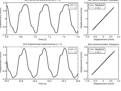
We now show results from real-time experimental substructuring tests using the inferred modal forcing relevant to the steady state flight case of 84knots. The robust transfer system design is applied as stated in 3.1 such that the test is commenced withγ = 0 to ensure robust stability. Typical experimental results are shown in Figure 7 for one continuous test, wherez is the numerical model displacement and x is the transfer system displacement. Figure 7(a1) shows the test between 6.6-7.6s forγ = 0 but after all transient behaviour has died away and the cancellation controller has achieved full delay compensation as can be seen from the synchronization subspace plot of Figure 7(a2). The robustness compensation is then phased out over a 5s period to give Figure 7(b1) which shows the test between 15.6-16.6s for the situation ofγ = 1, which is now real-time dynamic substructuring test using 100% of the experimental force. The algorithm is stable due to the high level of synchronization which is still achieved by the nominal model inversion as can be seen in Figure 7(b2).

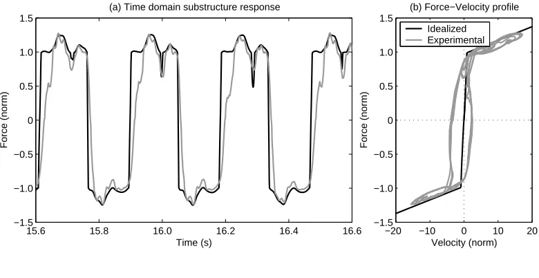
force being measured and shows how the idealized lag damper would behave at any given moment in time — in this case we know this is not actually representative of the true system.

It is clear from Figure 8(a) how the characteristic hysteretic behaviour of the real damper manifests itself in altering the idealized response. Therefore, the grey line (using the experimental force signal) can provide us with a far greater understanding of the vibrational characteristics of the energy being transmitted back into the helicopter fuselage than the idealized model. This is because it contains the same modal frequency content as would be found from the same lag damper on an actual helicopter in steady-state flight at 84knots (given the accuracy of the forcing term RFcode

i , which is the best

approxima-tion available for steady state trim condiapproxima-tions). This informaapproxima-tion can then be used to alter the characteristic dynamics of the lag damper by changing the tunable parameters (such as orifice size, bypass diameter, viscosity, relief valve arrangement and critical values etc.) to reduce damper loads at the critical harmonic frequencies (n±_{1 per revolution).}

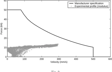
3.3 Accuracy of steady-state flight simulation

the whole profile being located well within the linear region. Thus, we can have high confidence that the global error for the experimental substructur-ing test is small and therefore this is demonstrative of the lag damper’s true dynamic characteristic in service during flight. Quantifying the accuracy of substructuring tests is an area of current research — see for example [29–31]

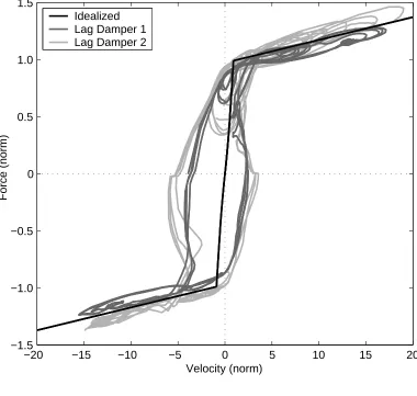
3.4 A comparison of two different lag dampers

It is clear that the lag damper has a significant influence on the blade dynamics and thus the vibrational energy transferred back into the fuselage. Therefore, as the EH101 is a five bladed helicopter all the lag dampers must be balanced such that no erroneous dynamics are created in the hub.

4 Stability of the substructuring algorithm

In this section we briefly discuss the stability of the substructuring algorithm. In particular we show how for a piecewise linear nonlinearity, such as the lag damper, estimates of critical delay can be obtained by extending the analysis of [32]. Figure 11 shows a simplified schematic representation of the blade and lag damper emulated system decoupled for each mode i= 1, . . . ,8. The nonlinear damper a4i and the nonlinear spring a5i are taken to be an approximation of

the physical lag damper. We can rewrite 1 in this simplified structure for the substructured system such that for each mode

a1iφ¨+a2iφ˙ +a3iφ+a4ixi˙ +a5ixi =a6i(RFicode), (18)

where, a1i,...,6i are predetermined coefficients (calculated from the parameters

defined in equation 1) for each mode i = 1, . . . ,8 (this data is commercially sensitive and therefore cannot be published), and again the state of the transfer system xi is described by a unit delayed response of the numerical model φi, such that xi = φi(t−_{τ). Solving this DDE will create eight separate critical}

limits, τc1,...,8.

To obtain an approximate stability analysis compressibility will be ignored,

a5 = 0. The damping coefficient of the idealized viscous damper can be

calcu-lated by simplifying the damper characteristics to being approximately linear (rather than nonlinear) piecewise smooth and reading off the resultant gradi-ents. This will produce two coefficients — c1 for when the blow-off valves are

both closed and c2 for when one is open. For linear systems the critical limit

represents the case where the idealized damper has both high damping and high stiffness, whereas c2 is the case for low damping and low stiffness. We

therefore must consider both situations to see which is the dominant case in terms of stability. Following [32] we rewrite equation 18 as

a1iφ¨+a2iφ˙+a4ic1,2φ˙(t−τ) +a3iφ = 0, (19)

for the unforced system.

We use DDE-BIFTOOL ([33]) to find real part of the characteristic root of the sixteen (eight for each damping case) critical delaysτciabove which the system is unstable. The absolute critical delayτcawill be taken as the smallest critical value and thus the delay magnitude which determines the absolute stability. Figure 12 shows the real part of the characteristic roots for equation 19 for the damping case ofc1 where both blow-off valves closed. The dominant mode (the

first root to cross the zero axis) is highlighted in bold and in fact represents the 7th_{mode which models the thirdlagmode. The smallest critical value is shown}

in the enlarged view in 12(b) and has a value of τc7 = 0.75ms. The smallest

critical value for the damping case of c2 is calculated to be τc8 = 6.34ms and

represents the 8th _{mode which modelstwist. Thus, the case where the blow-off}

valves are closed is shown to be the dominant factor in terms of stability, and sets the absolute critical value to be τca = 0.75ms.

and denominator (keeping the ratio the same to maintain the level of steady-state amplitude correction) the level of delay compensation is decreased until instability is observed at an approximate value of:

G′

n(s)−1 =

s + 245

241 , (20)

whereG′

n(s) is a reduced accuracy nominal model. At the dominant excitation

frequency of 3.5Hz this corresponds to 1.8ms difference in the magnitude of delay compensation gained from using the original nominal modelGn(s) given in equation 17. Therefore, as we know the original nominal model provides a very high level of synchronization this gives an approximate experimental critical limit of τc ≈ _{1.8ms rather than the approximated value of τca =}

5 Conclusion

In this paper we have shown how real-time dynamic substructuring can be used to test the dynamics of a lag damper when coupled to a rotor blade model. This in turn can give insight into the behaviour of the damper on the entire system rather than observing its dynamic characteristics in isolation.

A mathematical model for the rotor blade–lag damper system has been pre-sented, which has been used in previous studies to numerically model the system. In this work, the damper was tested experimentally and the mea-sured force used in the mathematical model instead of the previously assumed piecewise linear force profile. The whole process was carried out in real-time to achieve a real-time dynamic substructuring test.

A robust transfer system design was used to ensure that the experimental substructuring tests were stable and robust. The test results reveal the com-plexity of the damper dynamics when coupled to a modal rotor blade model. In particular they highlight the effects of hysteresis and valve dynamics on the rotor blade response and the vibration transfer to the rest of the helicopter.

and in utilizing adaptive damping strategies.

6 Appendix

The following expressions refer to the mathematical derivation in section 2.1. Further details can be found in both [6] and [23].

Tβ =              

cos(βB) 0−_sin(βB₎

0 1 0

sin(βB_{) 0 cos(β}B₎               , (21) Tζ =              

cos(ζB_{) −sin(ζ}B_{) 0}

sin(ζB_{) cos(ζ}B_{) 0}

0 0 1

              , (22) Tθ =              

0 0 1

0 cos(θB_{) −sin(θ}B₎

0 sin(θB_{) cos(θ}B₎               . (23) Tγ =              

cos(γB_)−sin(γB_{) 0}

sin(γB_{) cos(γ}B_{) 0}

0 0 1

Tδ =              

cos(δB_{) 0−sin(δ}B₎

0 1 0

sin(δB) 0 cos(δB)

              , (25)

Ti(1) = F CX(−θB(d−b)Y −(d−b)Z −(d−b)XβB)ωiD,

Ti(2) = F CX(θB(d−b)Z−(d−b)Y −(d−b)XζB)¯υiD,

T_i(3) = F CX(−_βB₍d−b_)YζB_(d−b) Z)ti_D,

Ti(4) = F CYυi¯D,

Ti(5) = −F CY(d−b)ZtiD,

Ti(6) = F CZωiD,

T_i(7) = F CZ(d−b_)Yti

D.

(26)

Acknowledgements

References

[1] B. Panda, E. Mychalowycz, and F. J. Tarzanin. Application of passive dampers to modern helicopters. Smart Materials & Structures, 5(5):509– 516, October 1996.

[2] D. L. Kunz. Elastomer modelling for use in predicting helicopter lag damper behavior. Journal of Sound & Vibration, 226(3):585–594, Septem-ber 1999.

[3] E. C. Smith, K. Govindswamy, M. R. Beale, and G. A. Lesieutre. Formu-lation, validation, and application of a finite element model for elastomeric lag dampers. Journal of the American Helicopter Society, 41(3):247–256, July 1996.

[4] W. Hu and N. M. Wereley. Magnetorheological fluid and elastomeric lag damper for helicopter stability augmentation.International Journal of Mod-ern Physics B, 19(7-9):1471–1477, April 2005.

[5] R. D. Eyres, P. T. Piiroinen, A. R. Champneys, and N. A. J. Lieven. Grazing bifurcations and chaos in the dynamics of a hydraulic damper with relief valves. SIAM Journal on Applied Dynamical Systems, 4(4):1076–1106, 2005.

[6] R.E. Eyres. Vibration Reduction In Helicopters Using Lag Dampers. PhD thesis, University of Bristol, UK, 2005.

[7] A. Blakeborough, M.S. Williams, A.P. Darby, and D.M. Williams. The development of real-time substructure testing. Phil. Trans. R. Soc. Lond. A, 359:1869–1891, 2001.

[8] D. Maclay. Simulation gets into the loop. IEE Review, 43(3):109–112, May 1997.

pseudody-namic tests. Earthquake Engineering and Structural Dynamics, 15:409–424, 1987.

[10] J. Donea, P. Magonette, P. Negro, P. Pegon, A. Pinto, and G. Verzeletti. Pseudodynamic capabilities of the ELSA laboratory for earthquake testing of large structures. Earthquake Spectra, 12(1):163–180, 1996.

[11] M. Nakashima, H. Kato, and E. Takaoka. Development of real-time pseudo dynamic testing. Earthquake Engng Struct. Dynam., 21:779–92, 1992.

[12] M. Nakashima. Development, potential, and limitations of real-time online (pseudo dynamic) testing. Phil. Trans. R. Soc. Lond. A, 359(1786):1851–1867, 2001.

[13] S. Y. Chu, T. T. Soong, and A. M. Reinhorn. Active, hybrid and semi-active structural control. John Wiley:Chichester, England., 2005.

[14] T. Horiuchi, M. Inoue, T. Konno, and Y. Namita. Real-time hybrid experimental system with actuator delay compensation and its application to a piping system with energy absorber.Earthquake Engng Struct. Dynam., 28:1121–1141, 1999.

[15] D.J. Wagg and D.P. Stoten. Substructuring of dynamical systems via the adaptive minimal control synthesis algorithm. Earthquake Engng Struct. Dynam., 30:865–877, 2001.

[16] A.P. Darby, A. Blakeborough, and M.S. Williams. Improved control algo-rithm for real-time substructure testing. Earthquake Engng Struct. Dynam., 30:431–448, 2001.

[17] A.P. Darby, A. Blakeborough, and M.S. Williams. Real-time substructure tests using hydraulic actuator. J. Engng. Mech., 125(10):1133–1139, 1999. [18] P.J. Gawthrop, M.I. Wallace, and D.J. Wagg. Bond-graph based

703, 2005.

[19] M.I. Wallace, D.J. Wagg, and S.A. Neild. An adaptive polynomial based forward prediction algorithm for multi-actuator real-time dynamic substruc-turing. Proc. R Soc. A, 461(2064):3807–3826, 2005.

[20] M.I. Wallace, A. Gonzalez-Buelga, S.A. Neild, and D.J. Wagg. Control techniques for real-time dynamic substructuring. Proc. IADAT Int. Conf. on Automation, Control and Instrumentation, Bilbao, Spain, 2-4 February, pages 56–60, 2005.

[21] W. D. Zhu, S. Pekarek, J. Jatskevich, O. Wasynczuk, and D. Delisle. A model-in-the-loop interface to emulate source dynamics in a zonal dc distribution system. IEEE Transactions on Power Electronics, 20(2):438– 445, March 2005.

[22] W. E. Misselhorn, N. J. Theron, and P. S. Els. Investigation of hardware-in-the-loop for use in suspension development. Vehicle System Dynamics, 44(1):65–81, January 2006.

[23] M. I. Wallace. Real-time dynamic substructuring for mechanical and aerospace applications: control techniques and experimental methods. PhD thesis, University of Bristol, 2006.

[24] R.E. Eyres, A.R. Champneys, and N.A.J. Lieven. Modelling and dynamic response of a damper with relief valve. Nonlinear Dynamics, 40:119–147, 2005.

[25] J.C. Houbolt and G.W. Brooks. Differential equations of motion for com-bined flapwise bending, chordwise bending, and torsion of twisted nonuni-form rotor blades. Technical Report, NASA, 1346, 1957.

[27] Y. N. Kyrychko, K. B. Blyuss, A. Gonzalez-Buelga, S. J. Hogan, and D.J. Wagg. Real-time dynamic substructuring in a coupled oscillator-pendulum system. Proceedings of the Royal Society A, 2005.

[28] P.J. Gawthrop, M.I. Wallace, S.A. Neild, and D.J. Wagg. Robust real-time substructuring techniques for under damped systems. Struct. Control and Health Monitoring, 2006. In Press.

[29] S.A. Mahin and P.B. Shing. Cumulative experimental errors in pseudo-dynamic tests. Earthquake Engng Struct. Dyn., 15:409–424, 1987.

[30] M.I. Wallace, D.J. Wagg, and S.A. Neild. Multi-actuator substructure testing with applications to earthquake engineering: how do we assess accu-racy? Proc. 13th World Conf. Earthquake Engineering, Vancouver, Canada, 1-6 August, pages 1–14, 2004. Paper No. 3241.

[31] B. Wu, H. Bao, J. Ou, and S. Tian. Stability and accuracy analysis of the central difference method for real-time substructure testing. Earthquake Engng Struct. Dyn., 34(7):705–718, 2005.

[32] M.I. Wallace, S.A. Neild, J. Sieber, D.J. Wagg, and B. Krauskopf. A delay differential equation approach to real-time dynamic substructuring.

Earthquake Engng Struct. Dynam., 34(15):1817–1832, 2005.

Figure Captions

• _{Figure 1: Close-up of the EH101 hub rotor system.}

• _{Figure 2: Cross-section of the hydraulic lag damper, including the relief}

valve orientations — Adapted from [6].

• _{Figure 3: Comparison of the damping characteristics of an idealized friction}

damper and an idealized hydraulic damper with relief valves — Normalized to critical relief valve parameters.

• _{Figure 4: Geometry of how lag damper is attached to the blade: “0”}

repre-sents the centre of the hub.

• _{Figure 5: Experimental test rig setup for the EH101 lag damper; Note, the}

standard size “hard hat” for scale.

• _{Figure 6: Experimental force-velocity damper profiles for dynamic}

identifi-cation — Normalized to upper tolerance limit critical value.

• _{Figure 7: An experimental substructuring test at a flight speed of 84knots}

— Normalized to mask commercially sensitive data.

• _{Figure 8: Force feedback during substructuring test from Figure 7 —}

Nor-malized to critical relief valve parameters.

• _{Figure 9: Estimated actuator capacity envelope for the actuator.}

Experi-mental data shown for the test of Figure 8 (5s test data).

• _{Figure 10: A comparison of two different lag dampers for an experimental}

substructuring test (a repeat of the test from Figure 7) — Normalized to critical relief valve parameters.

• _{Figure 11: Schematic representation of the blade and lag damper system for}

each modei= 1, . . . ,8.

• _{Figure 12: Real part of the characteristic roots for Figure 19 for the damping}

• _{Figure 13: Progression to instability as the magnitude of delay compensation}

is reduced (after approximately 8.6s the failsafe system kicks into action and stops the test automatically) — Normalized to mask commercially sensitive data.

Lag hinge "Fixed" end Central Hub

Flap hinge

Lag damper

xxxxxxxxxxxxxxxxxxxxxxxxxx xxxxxxxxxxxxxxxxxxxxxxxxxx xxxxxxxxxxxxxxxxxxxxxxxxxx xxxxxxxxxxxxxxxxxxxxxxxxxx xxxxxxxxxxxxxxxxxxxxxxxxxx xxxxxxxxxxxxxxxxxxxxxxxxxx xxxxxxxxxxxxxxxxxxxxxxxxxx xxxxxxxxxxxxxxxxxxxxxxxxxx xxxxxxxxxxxxxxxxxxxxxxxxxx

xxxxxxxxxxxxxxxxxxxxxxxxxx xxxxxxxxxxxxxxxxxxxxxxxxxx xxxxxxxxxxxxxxxxxxxxxxxxxx xxxxxxxxxxxxxxxxxxxxxxxxxx

xxxxxxxxxxxxxxxxxxxxxxxxxx xxxxxxxxxxxxxxxxxxxxxxxxxx xxxxxxxxxxxxxxxxxxxxxxxxxx xxxxxxxxxxxxxxxxxxxxxxxxxx

Piston

Chamber 2 Chamber 1

FLUID FLUID

Bypass Tube 1

Bypass Tube 2 Orifice

Blow-off valve 1

Blow-off valve 2

k1

k2

−10 −8 −6 −4 −2 0 2 4 6 8 10 −1.5

−1 −0.5 0 0.5 1 1.5

Velocity (norm)

Force (norm)

Friction Damper Hydraulic Damper

Standard size hard hat

(for scale) Vibration reduction beam

Damper Relief valves

100 kN load cell

Added mass

Pressure, Return and

Drain high pressure

pipes 2 servo

moog valves

100 kN capacity

steel support Temperature gauge (k-series

thermocouple)

15m/s electric fan

Internal LVDT Vertical motion

and vibration reduction support

Internal mechanical temperature compensation

Instron control box

−3 −2 −1 0 1 2 3 −1.2

−1.0 −0.8 −0.6 −0.4 −0.2 0 0.2 0.4 0.6 0.8 1.0 1.2

Velocity (norm)

Set Speed: 25mm/s (corresponding half−stroke: +/− 1.14mm)

Force (norm)

Upper Limit Lower Limit Profile

(a) Test No. 1

−60 −40 −20 0 20 40 60 −2.0

−1.5 −1.0 −0.5 0 0.5 1.0 1.5 2.0

Set Speed: 450mm/s (corresponding half−stroke: +/− 20.48mm)

Velocity (norm)

Force (norm)

Upper Limit Lower Limit Profile

(b) Test No. 2

15.6 15.8 16.0 16.2 16.4 16.6 −1.0 −0.5 0 0.5 1.0 Displacement (norm) Time (s)

(b1) Experimental substructuring (γ = 1)

−1.0 −0.5 0 0.5 1.0

−1.0 −0.5 0 0.5 1.0 Displacement (norm) Displacement (norm) (b2) Synchronization Subspace

6.6 6.8 7.0 7.2 7.4 7.6

−1.0 −0.5 0 0.5 1.0 Displacement (norm) Time (s)

(a1) Numerical substructuring (γ = 0)

−1.0 −0.5 0 0.5 1.0

−1.0 −0.5 0 0.5 1.0 Displacement (norm) Displacement (norm) (a2) Synchronization Subspace

z x

Idealized z vs x z

x

Idealized z vs x

−20 −10 0 10 20 −1.5

−1.0 −0.5 0 0.5 1.0 1.5

(b) Force−Velocity profile

Force (norm)

Velocity (norm)

15.6 15.8 16.0 16.2 16.4 16.6

−1.5 −1.0 −0.5 0 0.5 1.0 1.5

(a) Time domain substructure response

Time (s)

Force (norm)

Idealized Experimental

0 100 200 300 400 500 600 0

10 20 30 40 50 60

Velocity (mm/s)

Force (kN)

Manufacturer specification Experimental profile (modulus)

−20 −15 −10 −5 0 5 10 15 20 −1.5

−1.0 −0.5 0 0.5 1.0 1.5

Velocity (norm)

Force (norm)

Idealized Lag Damper 1 Lag Damper 2

a

φ

a_6i(MF_ic- LDMF_ic)

0 1 2 3 4 5 6

x 10−3 −100

−50 0 50 100 150 200 250 300 350 400

(a) Real part of characteristic roots

τ (s)

Re (

λ

)

0 0.5 1

x 10−3 −1

−0.8 −0.6 −0.4 −0.2 0 0.2 0.4 0.6 0.8 1

(b) Enlargement near τ

ca

τ (s)

Re (

λ

)

τ_ca = 0.75ms

7.4 7.6 7.8 8.0 8.2 8.4 8.6 −1.0

−0.5 0 0.5 1.0

Time (s)

Displacement (norm)

z x

0 50 100 150 200 250 300 350 400 450 500 −100

−50 0 50 100

Frequency (Hz)

Power (dB)

Stable Unstable