New parametrization method for dissipative particle dynamics

promoting access to White Rose research papers

White Rose Research Online

Universities of Leeds, Sheffield and York

http://eprints.whiterose.ac.uk/

This is an author produced version of a paper published in Journal of Chemical Physics.

White Rose Research Online URL for this paper: http://eprints.whiterose.ac.uk/3401/

Published paper

Travis, K.P., Bankhead, M., Good, K. and Owens, S.L. (2007) New

parametrization method for dissipative particle dynamics,Journal of Chemical Physics, Volume 127 (014109).

A new parameterization method for Dissipative

Particle Dynamics

Karl P. Travis

_{, Mark Bankhead}

_{, Kevin Good}

_{, and}

Scott L. Owens

1

Immobilisation Science Laboratory,Department of Engineering Materials,

University of Sheffield, Mappin Street, Sheffield S1 3JD, UK.

2

Nexia Solutions Ltd., Hinton House, Warrington, Cheshire, WA3 6AS, UK.

ABSTRACT

We introduce an improved method of parameterizing the Groot-Warren version of

Dissipative Particle Dynamics (DPD) by exploiting a correspondence between DPD and

Scatchard-Hildebrand regular solution theory. The new parameterization scheme widens

the realm of applicability of DPD by first removing the restriction of equal repulsive

interactions between like beads, and second, by relating all conservative interactions

between beads directly to cohesive energy densities.

We establish the correspondence by deriving an expression for the Helmoltz free

energy of mixing obtaining a heat of mixing which is exactly the same form as that for a

regular mixture (quadratic in the volume fraction) and an entropy of mixing which

reduces to the ideal entropy of mixing for equal molar volumes. We equate the

conservative interaction parameters in the DPD force law to the cohesive energy densities

of the pure fluids providing an alternative method of calculating the self-interaction

parameters as well as a route to the cross-interaction parameter.

We validate the new parameterization by modelling the binary system: SnI4/SiCl4,

which displays liquid-liquid coexistence below an upper critical solution temperature

around 140˚C. A series of DPD simulations were conducted at a set of temperatures

ranging from 0˚C to above the experimental upper critical solution temperature using

conservative parameters based on extrapolated experimental data. These simulations can

be regarded as being equivalent to a quench from a high temperature to a lower one at

constant volume.

Our simulations recover the expected phase behaviour ranging from solid-liquid

phase system. The results yield a binodal curve in close agreement with one predicted

using regular solution theory, but, significantly, in closer agreement with actual solubility

I.

INTRODUCTION

Dissipative Particle Dynamics (DPD) is one of the most promising methods for

modelling complex multi-phase materials developed in the last 20 years. It was developed

in the early 1990s by Hoogerbrugge and Koelman [1]

as a tool for simulating fluids from

the mesoscale (10-100 nm and 10-100 ns) to the continuum limit. The method represents

matter as a set of point particles, the distribution and density of which is determined by a

set of prescribed forces. Each of these point particles represents a "bead" of fluid. The

molecular structure of the fluid has been eliminated in the coarse grained description of

matter. The method shares features of both Molecular Dynamics and Lattice Gas

Automata and closely resembles the structure of a Brownian Dynamics algorithm, having

stochastic, dissipative and conservative forces. The conservative forces act to distribute

the beads in space as evenly as possible to minimise free energy. The dissipative force

represents friction and acts to reduce velocity differences between the beads. The

stochastic force represents the degrees of freedom that have been eliminated in the coarse

graining of matter. The magnitude of the stochastic and dissipative forces is coupled by

fluctuation-dissipation theorem and this acts as a system thermostat.

DPD has been improved several times since its introduction, most notably by

Español and Warren [2]_{, and then by Groot and Warren} [3]_{. The advantages of DPD are that}

the algorithm retains a very simple structure, it recovers hydrodynamic behaviour, and

can be used to study various types of fluid flow without the need for implicit solvents

the conservative forces, can be extended to multi-component systems using a simple

two-dimensional matrix of like-like and like-unlike terms.

A major weakness in the current application of DPD is that the method for

deriving the key interaction parameters has been, since its introduction by Groot and

Warren (GW), grounded in polymer science, through the application of Flory-Huggins

(FH) theory. It has become common practise when simulating mixtures using DPD to

treat AA type interactions as being no different to BB type interactions. Furthermore the

strength of these like-like bead interactions is often related to the isothermal

compressibility of ambient water. This choice of parameterization was merely suggested

by GW, presumably as a consequence of the correspondence between DPD and FH

theory. However, these suggestions have unjustifiably become inseparable from the

algorithm; applications abound in which this parameterization is effectively used,

including simulation of lipids [4]

block copolymers [5]

, vesicle formation of amphiphilic

molecules [6]

, surfactants [7]

and graft fluorinated co-oligomers [8]

. A rich range of phase

behaviour has been observed in many of these simulations but in all cases, quantitative

comparison with experiment is lacking; a DPD fluid will phase separate, but the

compositions of the resulting coexisting phases are necessarily symmetric and often

somewhat arbitrary. Clearly the phase compositions depend on the chemical details of the

various components and this must be taken into account if DPD is to become a serious

tool for modelling the phase behaviour of complex fluids.

In this paper we address the issue of parameterizing the DPD conservative forces.

We first demonstrate that GW DPD has essentially the same form of the free energy of

correspondence we then show how the entire conservative interaction matrix can be

determined using the cohesive energy densities of the pure components of a binary

mixture. We demonstrate that this method of parameterization is internally consistent by

considering the phase equilibria in the binary system, Stannic(IV)iodide (SnI4) /

tetrachlorosilane (SiCl4). The conservative force parameters for this system are obtained

using experimental solubility and heat of vaporisation data [9]_{. Our DPD simulations are}

broadly in agreement with both experimental solubility data and with the predictions of

regular solution theory; we observe solid-liquid and liquid-liquid coexistence, as well as a

single homogeneous phase close to the experimental upper critical solution temperature

(UCST). By contrast, we show that DPD simulations employing equal like-like bead

interactions do not give rise to the expected phase behaviour.

II.

THE DPD ALGORITHM

The original DPD method, first introduced by Hoogerbrugge and Koelman, has

been modified over the years, most notably by Pagonabarraga and Frenkel, who

introduced a density dependent conservative force into the algorithm [10]

. We prefer the

version of DPD as described in the paper by Groot and Warren (GW) based on its greater

simplicity [3]_{. We shall henceforth refer to this as the GW DPD algorithm. Since GW}

DPD has been described in detail elsewhere we give only a brief summary of it here. A

system of beads interact with each other as a result of pairwise additive forces comprising

of conservative forces, FC

, dissipative forces, FD

-7-

!

F_i =

(

)

# (1)

The conservative force is defined through

!

F_ijC =a_ij"C(r_ij) ˆ r _ij, (2)

where aij is the repulsive force parameter between particle i and particle j,

!

ˆ

r _ij is a unit

vector in the direction of rij, ω C

is a weight function and

!

r_ij =r_i"r_j. The weight function

is typically a linear ramp giving rise to very soft repulsive forces. It is the soft nature of

the conservative force that allows the use of very large timesteps in DPD compared with

molecular dynamics (MD).

The dissipative force depends on both the positions and relative velocities of the

particles, vij, through

!

F_ijD ="#$D(r_ij)

(

)

where ωD is the dissipative weight function, vij = vi – vj and the coefficient ζ controls the

strength of the dissipative force. The dissipative force models the viscous drag on a

particle due to the surrounding molecules of the fluid represented by the bead.

Thermal noise is introduced by means of a random force of the form

where σ is a parameter that determines the magnitude of the random pair force between

the particles, ωR

is the random force weight function, ξij is a Gaussian distributed random

variable, and Δt is the integration time step.

A requirement that the DPD system corresponds to a statistical mechanical

canonical ensemble [2]

places a restriction on the choice of weight function and

parameters for the dissipative and random force terms; the canonical distribution function

will only be a steady state solution of Liouville’s equation if the following relationships

are obeyed

ωD = (ωR)2

(5)

!

"2=2k_BT# (6)

We note here that the above conditions do not imply that DPD is a Hamiltonian system as

has been previously suggested [11]. There is no known Hamiltonian from which the DPD

equations of motion can be derived. The existence of a Hamiltonian is a sufficient but not

necessary condition for the phase space compression factor to vanish [12].

The combination of random and dissipative forces acts as a thermostat in DPD.

The random force term tends to heat the system up, while the dissipative term damps out

any increase in temperature.

!

"C(r_ij)="R(r_ij)= 1#rij/rc rij$rc

0 r_ij>r_c %

& '

(7)

where rc is the interaction range or cut-off distance which defines the length scale in

DPD. The dissipative weight function follows from Eq. (5).

III.

PARAMETERIZATION OF THE CONSERVATIVE FORCES

There are 3 parameters to determine in the DPD simulation of a 1-component

system of (monomeric) beads, a, σ and ξ, which become three m × m matrices upon

generalizing to an m-component mixture. The most important of these parameters is the

conservative force parameter since it contains all the chemical details of the substance to

be modelled; the noise and dissipative parameters are related respectively, to the system

temperature, and fluid viscosity. In what follows we shall assume literature values for the

damping and noise parameters and focus solely on the choice for the magnitude of the

conservative parameter [3]

.

For 1-component DPD simulations, Groot and Warren have shown that there is a

simple relationship between the conservative force parameter and the inverse isothermal

compressibility [3]

. This relationship is a consequence of the quadratic equation of state

for the DPD fluid. As DPD of 1-component systems is of limited interest we shall focus

on parameterization of mixtures. To keep the algebra simple, we restrict ourselves to

A. Free energy of mixing for a mixture of DPD particles

We now derive an expression for the free energy of mixing of two DPD fluids

starting from the equation of state. Both GW [3]

and Maiti and McGrother [13] have also

derived expressions for the free energy of mixing of binary DPD systems but these

authors work with a free energy density, taking a less detailed and transparent approach

than ours.

The pressure for a binary mixture of fluid components may be given in terms of

partial radial distribution functions by a straightforward generalization of the virial

equation, which follows from classical statistical mechanics of systems with pairwise

additive potentials [14]

!

P="k_BT#2$ 3 "

2

x2 g₁₁(r) 0 %

& du11(r) dr r

3

dr+2x(1#x) g₁₂(r) 0 %

& du12(r) dr r

3 dr

+(1#x)2 g22(r) 0 %

& du22(r) dr r 3 dr ' ( ) ) ) ) * + , , , , (8)

where x is the composition variable, gijare the partial radial distribution functions, ρ is the

total number density of the mixture, and uij(r) is the pair potential for species i and j.

If we now introduce the DPD conservative force expression (employing a linear

weight function) supplemented by the requirement that all species have the same

!

P="k_BT+2# 3 "

2

x2a₁₁ (1$r/r_c)r3g₁₁(r)dr

0

rc

% +2x(1$x)a₁₂ (1$r/r_c)r3g₁₂(r)dr

0

rc

%

+(1$x)2a₂₂ (1$r/r_c)r3g₂₂(r)dr

0 rc % & ' ( ( ( ( ) * + + + + (9)

We now transform the integrals by removing the dependence on the interaction

range by introducing the quantity

!

r =r/r_c. This now gives

!

P="k_BT+r_c4"2

[

]

where we have also defined the following parameters [13]:

!

"ij =

2#

3 (1$r )r 3

g_ij(r )dr 0

1

% . (11)

We note that Eq. (10) describes a quadratic equation of state. As pointed out by

Pagonabarraga and Frenkel [10]

, such an equation of state will be produced no matter what

choice of weight function is employed. For this reason, the GW form of DPD is

inadequate for modelling vapour-liquid equilibria in pure substances.

To a good level of approximation the α’s can be taken to be independent of the

total density [13] (by virtue of removing the dependence on rc) and furthermore that α 11 ≈ α 12 ≈ α 22≡α. This last identity is not as serious an assumption as might be thought; it

!

P="k_BT+r_c4"2#

[

]

An equation of state of this form may be integrated using the general limit

theorem [15] to give the Helmoltz free energy of the binary mixture [16]

!

A_mix = P"nTRT

V # $ % & ' ( V )

* dV"RT n_iln V

n_iRT

i

+ + n_i

(

)

i

+ (13)

where the lower case letters denote extensive quantities per mole of substance while the

‘0’ superscripts refer to a pure ideal gas reference state. In particular, nT is the total

number of moles, s and u are the molar entropy and molar internal energy, respectively.

Substitution of Eq. (12) (the DPD equation of state) into Eq. (13) gives the

Helmoltz free energy per mole of mixture, Amix /nT, as

!

A_mix

n_T = "RT x#_i iln V

n_iRT +#_i xi ui 0

"Ts_i0

(

)

n_T VPvir

$

% dV (14)

where Pvir is defined by

!

P_vir = rc 4_n

T2NA2"

V2 x

2_a

11+2x(1#x)a12+(1#x)2a22

Evaluating the definite integral in Eq. (14) gives the following expression for the free

energy per mole of mixture

!

A_mix

n_T ="xRTln V

n₁RT "(1"x)RTln V

n₂RT +x u1 0

"Ts₁0

(

)

(

)

4_n

TNA2#

V x

2

a₁₁+2x(1"x)a₁₂+(1"x)2a₂₂

[

]

(16)

The free energy of mixing, AM

, is obtained by subtracting the free energies of the

two pure components from that of the mixture [17]:

!

AM n_T =

A_mix n_T "x

A₁

n₁ "(1"x) A₂

n₂ (17)

where A1 and A2 are the free energies of pure components 1 and 2 respectively. These

pure component free energies can be obtained from the free energy of the mixture by

using the molar volume of the pure species in place of the total molar volume and setting

the mole fraction x to unity and zero for species 1 and 2, respectively. These free energies

per mole of each substance are

!

A_i

n_i ="RTln V_i n_iRT + ui

0 "Ts_i0

(

)

4_n

iNA2# aii

V_i , (18)

in which the subscript i refers to substance 1 or 2. The Helmoltz free energy of mixing,

AM

!

AM

n_T =xRTln xv1 v " # $ % &

' +(1(x)RTln (1(x)v2

v " # $ % & '

+rc

4

N_A2)

v x

2_a

11+2x(1(x)a12+(1(x)2a22

[

]

(x rc

4

N_A2) a₁₁

v₁ ((1(x)

r_c4N_A2) a₂₂ v₂

(19)

in which we have introduced the molar volumes in place of the extensive total volumes.

The first two terms on the rhs of Eq. (19), having an explicit temperature dependence,

may be regarded as the entropic contribution to the free energy of mixing. Introducing the

volume fractions

!

"₁=V1

V # x₁v₁

v #", (20)

in which we have assumed (as in regular solution theory) that there is no volume change

upon mixing (partial molar volumes are equal to the molar volumes). This leads to an

entropy of mixing per mole of the mixture of

!

sM

R ="xln#"(1"x)ln(1"#) (21)

Eq. (21) is very similar to the expression for the ideal entropy of mixing, becoming

exactly so when the volume fractions and mole fractions coincide, which happens for

The remaining contribution to the free energy of mixing, which we shall loosely

call the excess free energy of mixing (excess properties of mixing are usually defined

relative to the properties of an ideal mixture at the same temperature, pressure and

composition) is from Eq. (19)

!

AE n_T ="rc

4_vN

A2# a₁₁ v₁2 "2

a₁₂ v₁v₂+

a₂₂ v₂2 $

% & &

'

( )

) *(1"*) (22)

We note here that Groot and Warren derived an expression for the free energy of

mixing in which the entropy term was ideal and the heat term was given in terms of mole

fractions [3]

, while Maiti and McGrother did not consider the entropy of mixing and also

derived a heat of mixing which was quadratic in mole fraction, not volume fraction [13].

B. Mapping DPD onto Regular Solution Theory

Equation (22) derived in the last section has almost the same form as the free

energy of mixing derived by Scatchard [18] and Hildebrand [19] for systems described as

regular mixtures by Hildebrand [20]. Hildebrand defined a regular solution as one in which

the excess entropy, SE_{, and excess volume, V}E_{, of mixing are both zero. Regular mixtures}

display positive deviations from Raoult’s law and are typically formed from components

with non-polar molecules (essentially ignoring dipolar and hydrogen bonded forces

between molecules). Scatchard and Hildebrand obtained the following equation for the

!

uE =v(c11+c22"2c12)#(1"#)$gE (23)

where the last identity in Eq. (23) follows from VE = SE

= 0, and the parameters c11 and c22

are the cohesive energy densities of the two pure liquids defined by

!

c "#vapu

vL (24)

in which Δvapu is the molar internal energy of vaporisation and v

L _{is the molar volume of}

the liquid. The main assumptions used to derive Eq. (23) are that VE

= 0 and that the

energy of the binary mixture can be expressed as a quadratic function of the volume

fraction [17]. Eq. (23) can also be viewed as the leading term in the Redlich-Kister

expansion of the excess free energy of mixing where the 3 terms in parentheses are then

lumped together to form a new empirical constant, A. The assumption of zero excess

entropy is true for only a few non-ideal mixtures and for this reason, the term ‘regular

mixture’ is reserved in more modern treatments for those mixtures for which the constant

A in the Redlich-Kister expansion is temperature independent [21]. Nevertheless, many

mixtures can be adequately represented by Scatchard and Hildebrand’s regular solution

theory due in part to a fortuitous cancellation of errors. Their theory is also quite simple

to understand and provides meaningful physical insight, which is lacking in the more

empirical treatments of the free energy of mixing. It is advantageous to make a

between the conservative interaction parameters, a11 and a22 and the cohesive energy

densities, c11 and c22.

GW [3]

and Maiti and McGrother [13] used similar arguments to develop equations

for the free energy density of DPD particles in a binary mixture. They arrived at a similar

expression (though see earlier note on this) to Eq. (22), suggesting a correspondence with

the Flory-Huggins lattice theory of polymeric solutions. Through our detailed derivation

of the thermodynamics of mixing we have shown that the correspondence is closer to that

of regular solution theory. It should be noted that in Flory-Huggins theory, the same

form of the heat of mixing (as in RST) is employed; the significant difference lies in the

treatment of the entropy of mixing. By focussing on FH theory both sets of authors

missed the link between the like-like interaction parameters and cohesive energy density.

Instead, they set a11 = a22 whose value they suggested could be determined from the

isothermal compressibility (as for the 1-component DPD case). This was an unfortunate

oversight; the use of equal like-like interactions is only justified in a few special cases

and will not in general give rise to the expected phase behaviour.

The cross interaction parameter c12 was related to c11 and c22 in Hildebrand’s

theory by a geometric mean,

!

c₁₂= c₁₁c₂₂ (25)

which has some physical justification for non-polar molecules based on London’s

following expression for the excess free energy of mixing in regular solution theory

(RST),

!

gRSTE ,

!

g_RSTE =v"(1#")

(

)

, (26)

in which δ1 and δ2 are now the square roots of the pure component cohesive energy

densities, or the Hildebrand solubility parameter. Comparing Eq. (22) with Eq. (26)

gives the following mapping between the DPD parameters and cohesive energy densities,

!

"1#"2

(

)

[

]

The negative sign on the rhs of Eq. (27), which arises from the use of a purely repulsive

conservative force, is significant; without it there would be a one to one correspondence

between a11 and δ1, and between a22 and δ2 with a12 then given by the geometric mean of

a11 and a22. Instead we must regard Eq. (27) as a definition of a12. This is possible since all other parameters are in principle known: a11 and a22 could be determined from pure

component compressibility data as suggested by GW, while α has been determined by the

same authors to be approximately 0.1 for DPD densities ρrc

3 _{> 3. Alternatively, we}

propose that a11 and a22 be determined from Hildebrand solubility parameters via the

following argument. The cohesive energy density is approximately equal to the volume

!

E_coh V "#

2

$%U

%V (28)

This relationship is exact for a van der Waals fluid. The internal pressure is given by the

thermodynamic equation of state as

!

"U "V =T

"P

"T #P (29)

The only explicit temperature dependent part of the DPD pressure equation of state

involves the ideal gas contribution, therefore the internal pressure is just the virial term

with its sign reversed. Hence using Eqs. (15, 28 & 29) and setting the mole fraction to be

1 or 0, we obtain

!

a_ii= "i 2

#$i2rc4

(30)

Solubility parameters have been determined for a wide range of substances

including solids. For a substance which is a solid at the temperature of interest, one uses

the molar volume of the subcooled liquid to calculate the solubility parameter [20]. The

most reliable method of calculating these parameters is to use Eq. (24) in which the heat

of vaporisation is required [20]. Various other methods are available for calculating or

estimating solubility parameters including estimation from the Hildebrand rule, from

by Hildebrand and Scott [20]. To complete the parameterization of the conservative forces

one must specify the value of rc, which we will discuss in the following section.

IV

DPD SIMULATION OF A 2-COMPONENT MIXTURE

To validate the new parameterization of the conservative forces we have

conducted a series of DPD simulations in which we have modelled the phase equilibrium

of a 2-component mixture of inorganic species. We have chosen to study the system

SiCl4/SnI4 for several reasons: First, it is far removed from polymer systems and therefore

illustrates the wide applicability of our new parameterization; Second, this system is

known to behave as a regular mixture; Third, experimental solubility data are available

for this system; Finally, the mixture phase-separates below 140˚C, forming two liquid

phases with a non-symmetric composition, providing a stern test of the new

parameterization.

A. Experimental data

Hildebrand and Negishi have determined the solubility of SnI4 in a SiCl4 solvent

at a set of temperatures ranging from 0.2 ˚C to just below 140 ˚C [9]

. From this data they

derived a set of values for the square difference in solubility parameters,

!

"SnI₄ #"SiCl₄

(

)

at various temperatures by applying the RST derived equation for the activity coefficient

obtained by other authors, while the ideal solubilities of solid SnI4 in liquid SiCl4 were

calculated using measured values of the heat of fusion and molar excess heat capacity of

the liquid over the solid phase.

We have used Hildebrand and Negishi’s derived

!

"SnI₄ #"SiCl₄

(

)

with Eq. (26) to calculate the excess free energy per mole of the mixture as a function of

temperature. By adding the entropic contribution, we calculated the molar free energy of

mixing. This data was then used with the thermodynamic software code, Thermo-Calc to

determine the locus of coexisting solubilities (the binodal phase boundary). The

calculated phase boundary is a skewed parabola with a maximum at about 144˚C,

occurring at a composition of around 44 mole percent of SnI4. It should be noted that the

right hand branch of the T-x diagram is obtained by extrapolating far beyond the range of

experimental solubility data and must therefore be seen only as a guide (see later plot in

Fig. 4). The upper critical solution temperature (UCST) is overestimated by

Thermo-Calc; this can be taken as a measure of the error in applying RST to this system

To conduct our DPD mixture simulations we require a set of data for the

solubility parameters of each of the pure components as a function of temperature in

order to fully parameterise the conservative force matrix. There are several ways to

proceed from here but we have chosen to do the following: (1) Calculate a value of the

solubility parameter for SiCl4 at 25 ˚C and then extrapolate to obtain values at the other

temperatures; (2) The solubility parameters for SnI4 are then calculated using these values

together with Hildebrand and Negishi’s values for

!

"_SnI4 #"_SiCl4

(

)

An alternative approach would be to calculate directly the SnI4 solubility

parameters using extrapolated vaporization enthalpies. However, SnI4 is a solid across

much of the temperature range and hence introduces the added difficulty of having to

determine values for the molar volume and heat of vaporization for the subcooled liquid.

The first step in our chosen scheme involves calculating the solubility of SiCl4 at

25 ˚C. This we determined from a tabulated value of the standard enthalpy of

vaporisation at this temperature, Δvaph 298

of 29.7 kJ mol-1

[22], together with the equation

!

"SiCl₄ #

$vaph[SiCl4]%RT

v_SiCl 4 & ' ( ( ) * + + 1/ 2

, (31)

which follows from Eq. (24) upon assuming the vapour behaves as an ideal gas [20]. A

more sophisticated calculation should involve the compressibility factor of the vapour [20].

Solubility parameters at the remaining temperatures of interest were also determined

using Eq. (31), but now with values of the enthalpy of vaporisation estimated at these

temperatures from Kirchhoff’s law,

!

"h(T₂)="h(T₁)+ "c_pdT

T1

T2

# (32)

where cp is the constant pressure molar heat capacity and T1, T2 are the two temperatures

of interest. For the particular case of the heat of vaporisation, provided the heat capacity

of the liquid and vapour phases can be taken to be approximately independent of

!

"_vaph(T₂)="_vaph(298K)#"c_p(T₂#298.15K) (33)

where Δcp is now the difference between the molar heat capacity of the liquid and vapor

phases, and the reference temperature is taken to be 298 K. Taking a value for

Cp(SiCl4, liq) = 145.3 J K -1

mol-1

and Cp(SiCl4, gas) = 90.3 J K -1

mol-1

[22] gives

ΔCp = 55 J K -1

mol-1

.

The next stage of the parameter determination is to estimate a set of solubility

parameters for SnI4. This was achieved by using

!

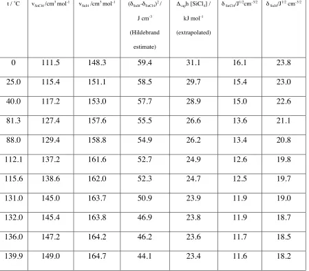
"_SnI4 ="_SiCl4 +

(

)

The values we obtained for the heat of vaporization and solubility parameters are

collected in Table 1.

B. DPD simulation details

DPD simulations are commonly conducted using a system of dimensionless units.

The interaction distance, rc is an obvious choice for the unit of length while the mass of

the DPD beads can be used as the unit of mass. One choice for the unit of energy is the

value of kBT. With these three choices, the timestep is then determined. Another

possibility would be to choose a suitable unit of time, which would then set the energy

scale. We have opted for the former method in view of its simplicity. In this system we

example, the dimensionless number density,

!

"="r_c3, while the repulsive parameters

become,

!

a _ij=a_ijr_c/

₍

₎

Defining an energy scale based on kBT means the repulsive parameters become

temperature dependent and further, that the DPD simulations are all conducted at unit

temperature; separate DPD simulations must be conducted to explore different real

temperatures. There is an effective lower limit to the reduced DPD density; GW

determined that

!

" #3 in order for a quadratic equation of state to be recovered that is independent of the magnitude of the conservative force parameter. Employing higher

values of density than this will increase the computing overheads of a simulation hence it

is desirable to keep it as close to 3 as possible. Fixing the reduced density effectively sets

the value of rc since it is then given by the cube root of three times the reciprocal of the

density of the substance of interest. Note that this interaction length can be increased but

only at the cost of increasing the value of the reduced density. Some authors introduce an

extra parameter involving the number of atoms that a DPD bead is supposed to represent

to act as an extra scaling factor on rc, allowing it to increase, while keeping the reduced

density constant. We have chosen not to adopt this approach and hence our version of

DPD does not run into problems such as those discussed in the article by Pivkin and

Karniadakis, in which the DPD fluid solidifies beyond a certain level of coarse graining

[23]. This leaves open the question of what the DPD beads represent. We have taken the

view that the beads are blobs of fluid (see the article by Kim and Phillips for a very

illuminating and insightful description of what the DPD particles represent [24]). By

insisting that the beads all have the same interaction range, rc, all we are saying is that

conditions or different thermodynamic states of the same substance, the volume of each

bead simply encloses a different number of atoms or molecules; for a vapor there will be

far fewer molecules in such a control volume than for the same substance under

conditions in which it is a liquid. Clearly, in this example, the ‘vapor’ beads must have a

softer interaction than the ‘liquid’ beads, but this is accounted for in the value of the

conservative force parameter, which will be greater (more repulsive) for the “liquid”

beads. Beads representing lumps of a solid phase will have even higher repulsive

parameters due to the higher density of the underlying atomic units. It is useful to think of

the DPD beads as representing “spheres of influence” of the underlying molecules with a

size that is characterised by a diameter, rc.

For simplicity, our mixture simulations have all been conducted at the equimolar

composition. The mixture volume is then given by the arithmetic mean of the pure

component molar volumes (we assume here, as in RST, that the partial molar volumes

differ very little from the pure component molar volumes). The number density of these

mixtures at the various temperatures is then calculated by multiplying the reciprocal

volume of one mole of the mixture (its molar density) by the Avogadro constant.

In order to satisfy both the requirement of having a constant rc for all our

simulations and having a reduced density as close as possible to 3, we have fixed the

value of rc based on the largest value of any pure component molar volume across the

range of temperatures under investigation. In our case the highest value of molar volume

occurs at the temperature of 139.9 ˚C for SiCl4. This gives a value of rc = 0.9362 nm. With this choice, the reduced density of all our mixtures stays close to 3 and never dips

Once the values of the dimensionless solubility parameters have been determined

using the above choice for the interaction range, the repulsive parameters are then

obtained with the aid of Eq. (30) together with the dimensionless version of Eq. (27). The

variation of these parameters with temperature is shown in Fig. 1. The graph shows that

the parameters decrease with increasing temperature, as expected. Furthermore, it can be

seen that the parameters for a pair of interacting SnI4 beads are greater than for SiCl4

beads. This is sensible since SnI4 is almost 3 times as dense as SiCl4 at 25 ˚C, being a

solid at this temperature. The mixing term falls somewhere in between the two like-like

parameter values.

Simulations were solved using a DPD code that implements the standard GW

method supplied by Accelrys Inc. [25]. Cubic boxes, with imposed 3D periodic boundary

conditions, containing random arrangements of between 24400 and 30890 beads were

simulated for an equilibration phase of 100,000 steps followed by a production phase

comprising of 100,000 steps. Equilibrium was deemed to have been achieved when the

cumulative average temperature and pressure reached a plateau. A time step of

!

"t =0.02

was used throughout and the values of the noise and damping coefficients were

!

" =3

and

!

" =4.5, respectively. The DPD simulations may be thought of as being equivalent to

a quench from a high configurational temperature (random arrangement of beads) to

thermodynamic equilibrium at the temperature of interest, under constant volume

V.

RESULTS AND DISCUSSION

By viewing snapshots taken from the simulations it was possible to discern clear

SiCl4 rich zones, and SnI4 rich zones at low temperatures indicative of the early stages of

phase separation. As temperature approached the experimental critical point the

snapshots showed little evidence of any phase separation. Due to the ambiguity of

snapshots we have chosen not to present them in this manuscript. To determine the

composition of two coexisting phases we could perform the simulations in an elongated

box using a large value of the Flory-Huggins coefficient to promote phase separation with

a stable planar interface as used in the paper by GW. However, we have chosen not to

follow this method because (a) it is not necessary to wait until complete phase separation

takes place, (b) we wish to show that the DPD mixture will phase separate at the points

where the experimental system phase separates (which should occur if the

parameterization is correct) and not simply at some mean field value.

As remarked above the simplest approach to analysing phase equilibria without

ensuring one has a planar interface entails calculating distribution functions of local

densities and compositions. This method relies on the fact that these local distributions

reach equilibrium much faster than the time taken to achieve global equilibrium.

To use this method, one first constructs a histogram of the local density; different phases

will then appear as separate peaks in the histogram. The local density can be calculated

by dividing up the simulation box into a smaller number of cubes of equal volume and

then simply counting the number of beads that lie within the region enclosed by each one.

between them. For a relatively small total number of particles, a significant number of

these will reside in the interfacial region. The naïve local density approach described

above will lead to a smeared out histogram as a result of the contributions of the

sub-cubes located in the interfacial region [26]. A better strategy than this involves identifying

those sub-cubes which reside in the interfacial region, and removing these from the

statistical analysis. Gelb and Müller have devised a simple scheme by which the phase

boundary can be easily located [26]. Their method entails forming a histogram of local

coordination number or better still, a histogram of component specific coordination

number. This histogram is obtained by first selecting a cutoff distance, then determining

the number of neighbours (or neighbours of a given species) of each bead in the

simulation box. From the histogram that is produced, one may determine a criterion for

deciding which beads belong to the interfacial region. For a two phase system, such a

histogram will be bimodal; the higher density phase will be characterised by beads with

relatively high coordination numbers, while the lower density phase will give rise to a

peak at relatively low coordination numbers. Beads that lie in the interfacial region will

be characterised by having coordination numbers intermediate between the average

values for the two phases. Having defined a region of coordination numbers that

constitutes membership of the interfacial region, one then determines which of the

original set of sub-cubes are to be excluded from the analysis. We have followed Gelb

and Müller by deeming a sub-cube to be interfacial if more than 30% of its constituent

beads are themselves interfacial by virtue of the coordination number analysis. It should

be stressed that the above local density scheme is carried out post-process and in no way

The choice of which cutoff distance to employ is somewhat arbitrary. However,

choosing a value too low will give poor resolution of the two coexisting phases while too

high a value will give an interface that is too “thick”. The choice for the number of

sub-cubes to use in the local density calculation is also somewhat arbitrary. In our simulations

we typically used a discretization of 7×7×7 sub-cubes but the highest discretization used

8×8×8 cubes. These numbers were determined by trial and error – too few cubes gave

poor resolution of the two peaks in the density profile while too high a value resulted in

too few particles per cube to calculate a meaningful average local density. For the

coordination analysis we used cutoff distances ranging from 1.25 at 0 ˚C to 2.0 at 131 ˚C.

We opted to calculate the coordination number of SiCl4 beads around any given bead

regardless of its own identity. This choice gave a clearer separation of the peaks in the

histogram for a smaller cutoff than one based upon a “species blind” coordination number

histogram. During the DPD simulations, several snapshots were taken at equally spaced

intervals of time. Our statistical analysis was carried out on each of the snapshots and the

results averaged in the final analysis.

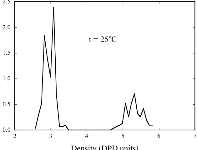
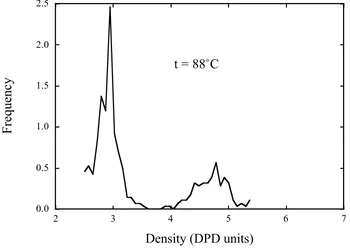
A set of density histograms are shown in Figs. 2a-e. These histograms have been

obtained via the method outlined above. The histograms below 140 ˚C are bimodal with a

peak centred on a density of around

!

"=3, largely independent of temperature and a

second peak that moves inwards towards lower densities with increasing temperature. At

the lowest temperature plotted (0 ˚C) the second peak lies at a density of around 6, a

factor of two greater than the mean density of the 1st peak.

We can interpret the results plotted in Fig. 2 in the following way. As temperature

phase will become less dense (when measured in DPD units) because the SnI4 beads are

much more repulsive between themselves and the SiCl4 beads, than the SiCl4 beads are

between themselves. This causes the SiCl4 rich phase to expand in volume, thus lowering

its density. Once all of the solid SnI4 has melted we are left with two coexisting liquids

with densities that are not sufficiently different to separate by the local density histogram

method we have employed. As the critical temperature is reached, it becomes impossible

to discern two phases; plots of coordination number show only a single peak no matter

what cutoff is chosen. This is not a concern in the present context since we are not

interested in accurately determining the critical temperature or composition. The species

coordination number histograms are shown in Fig. 3 for sub-set of the temperatures

studied. This plot illustrates how the peaks merge together as the critical temperature is

approached. To resolve the phases in the vicinity of the critical point requires the use of a

more sophisticated technique than we have employed. Methods which are based on

topology, such as the use of ring statistics frequently employed in simulations of network

glasses, may be useful in this context.

Once the two coexisting phases have been identified from an inspection of the

local density histogram, the mean values of the density and composition of each phase

can be determined. For a given temperature we obtain two values for the composition

which can then be plotted to yield the binodal phase boundary. Each of these points is the

result of averaging the composition from 5 individual snapshots taken at regular intervals

during the last phase of the DPD production runs. Errors were calculated based on one

standard deviation from the mean values and were typically smaller than the plot

that we have made in the parameterization (use of constant heat capacities, assumption of

ideal vapour phase, assumption of zero volume change on mixing, errors in the original

experimental data etc.).

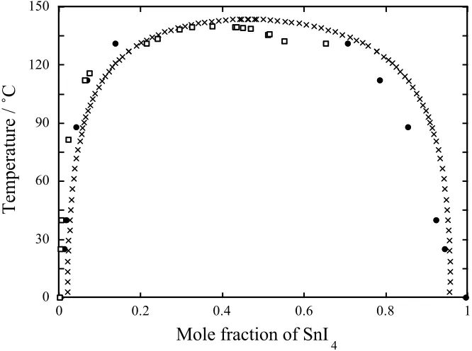
The results from our analysis (solid circles) are plotted against the Thermo-Calc

generated phase boundary data (crosses) and Hildebrand and Negishi’s experimental

solubility data on a T-x diagram shown in Fig. 4. It is clear from Fig. 4 that the results for

the SiCl4 rich phase are in excellent agreement with the experimental data until we enter

the two liquid region where the single DPD data point in that regime appears at too high a

temperature. We attribute this to the difficulty in resolving the two liquid phases using

our simple histogram method. The Thermo-Calc results are shifted to the right of the

DPD and experimental data. This systematic discrepancy is the result of the

approximations employed in RST. Lack of experimental data on the SnI4 rich phase

mean that the DPD and Thermo-Calc data are at best a crude guide to the true phase

behaviour. Nevertheless, the agreement between Thermo-Calc and DPD is encouraging.

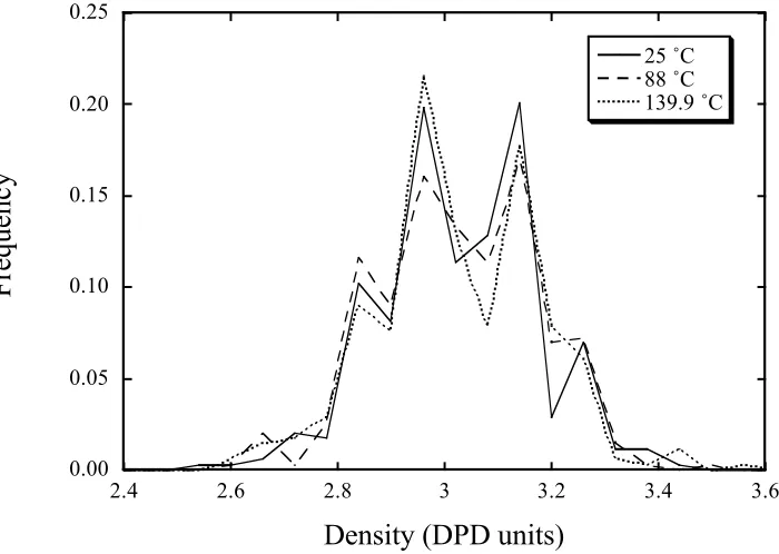
Finally we have conducted three additional DPD simulations using the

parameterization scheme commonly employed by many DPD practitioners. For these

simulations we set

!

a ₁₁=a ₂₂=a =25 but determined the value of

!

a ₁₂ using the RST

calculated heat of mixing (equivalent to using what GW call the Flory-Huggins

coefficient). Using our Eq. (27) we may write (in the spirit of these other DPD authors),

!

"₁#"₂

We carried out these extra DPD runs at temperatures, 25 ˚C, 88 ˚C and 139.9 ˚C. Using

Eq. (35) together with the solubility parameters taken from Table 1, we obtained the

following respective set of values for

!

a ₁₂: 31.4, 30.0, 28.5 using a

!

" = 3 and a value of rc

= 0.87 nm. Random configurations of equimolar mixtures of beads were equilibrated in

exactly the same manner as in our main simulation work (system size was 24000 beads in

each case). After a production phase, the snapshots obtained from the last trajectory were

stored to disk and these were then analysed.

All three snapshots looked very similar and it was impossible to discern any phase

separation by visual inspection. Local coordination number histograms were all single

humped regardless of the cutoff employed. Local density histograms were therefore

calculated without the clean-up procedure described earlier. These histograms are plotted

in Fig. 5 for a discretization of 7×7×7 sub-cubes. It is clear from Fig. 5 that there is no

evidence for the existence of two coexisting phases at any of the 3 temperatures. Wijmans

and co-workers determined that for the system with

!

a ₁₁=a ₂₂= 25 and a DPD density of

3, phase separation cannot be expected until

!

a ₁₂ is somewhere between 28.5 to 31.4 in

value[27]. Since this value is larger than the ones we used in our three simulations it would

seem an unfair criticism. However, the point is that if DPD is to be taken seriously, then a

well parameterised model must predict phase separation at a point coincident with

experiment. Evidently, this is not true of the established parameterization method.

A parameterization of soft-core potentials typically employed in DPD and based

on equal diagonal elements of the force parameter matrix, is known to yield fluid-fluid

phase separation in binary mixtures. Such an approach is appealing since it can act as a

Evans [29]). However, these parameterizations are tied to mean field Flory-Huggins theory

and may only give rise to symmetric coexistence curves. Maiti and McGrother added a

proof of why

!

a ₁₁=a ₂₂, based on a thought experiment [13]. This proof is based on the

conjecture that both components must have equal molar volumes, which is not true in

general and seems to be a consequence of the Flory-Huggins lattice theory. It is clearly

more desirable to have a parameterization method which is mapped to real experimental

data, is not restricted to polymers or mean field theory, and can be used in a predictive

sense.

VI.

CONCLUSIONS

We have introduced a significantly improved method of parameterizing the

Groot-Warren formulation of Dissipative Particle Dynamics (DPD) by exploiting a

correspondence with Scatchard-Hildebrand regular solution theory. Using

thermodynamic arguments we have shown that the free energy of mixing of a DPD

mixture has almost the same form as that derived using RST. The central difference lies

in the entropy of mixing. In the case of DPD, we find that the entropy of mixing is greater

than that of an ideal mixture when the molar volumes of the two components are not

equal. In fact, our entropy of mixing expression is formally identical to one derived by

Hildebrand for athermal mixtures using the concept of free volume, and also in

agreement with the entropy of mixing of polymer solutions derived by Flory [20]. RST, on

the other hand, assumes the excess entropy of mixing is zero. Significantly, the heat of

function of the volume fractions. Using this correspondence we have established that the

self-interaction parameters are related to the cohesive energies of the pure fluids and have

derived a method of obtaining them. This is a significant departure from what has

previously been practised in the DPD literature, where the self-interaction terms are

typically taken to be equal. Some exceptions have been made to this rule, when

simulations have involved molecules with hydrophilic heads and hydrophobic tails for

example, but the variation in parameters has been somewhat arbitrary. By contrast, we

now provide a physical basis for establishing the magnitude of the self-interaction

parameters. For the cross interaction parameters we do not take the more drastic step of

assuming they obey a geometric mean combining rule as per RST. Instead, we used an

RST-derived heat of mixing (which does involve the use of the geometric mean rule) to

define these parameters. This may seem like a subtle difference, but it means DPD is not

intimately tied to RST; experimental data on heats of mixing could be used in place of

one based on a geometric mean combining rule. It is also worth noting that molecular

simulation methods, such as Molecular Dynamics and Monte Carlo, frequently employ

the Lorentz-Berthelot combining rules, and thus are not immune from this problem,

which arises from the lack of an accurate theory of the interaction energy of a pair of

chemically dissimilar molecules.

We have validated our new parameterization scheme by modelling the binary

system: SnI4/SiCl4, which displays liquid-liquid coexistence below an upper critical

solution temperature around 140˚C. A series of DPD simulations were conducted at a set

of temperatures ranging from 0˚C to above the experimental upper critical solution

These simulations can be regarded as being equivalent to a quench from a high

temperature to a lower one at constant volume.

Our simulations recovered the expected phase behaviour ranging from solid-liquid

coexistence to liquid-liquid co-existence, eventually leading to a homogeneous

single-phase system. The results yield a binodal curve in close agreement with one predicted

using regular solution theory, but, significantly, in closer agreement with actual solubility

measurements, suggesting the DPD system is an improvement over RST. This last point

means that DPD should not be regarded as a solver for RST – if that were the case, DPD

would be pointless.

To further illustrate the importance of allowing the self-interaction parameters to

differ from each other in magnitude, we conducted a series of DPD simulations using the

commonly practised procedure of setting these parameters to be equal in magnitude.

These simulations demonstrated that the known phase behaviour of SnI4/SiCl4 could not

be recovered.

Regular Solution Theory provides a very convenient framework in which to

parameterize the whole conservative force matrix. Particularly useful is the ability of RST

to predict the behaviour of mixtures from a knowledge of only the pure components.

Furthermore, RST is easily extended to treat multi-component mixtures. The

correspondence between DPD and this more general form of RST should be preserved,

opening up DPD to simulating more complex solutions.

RST does have some drawbacks and we now consider some of the more serious

ones, indicating how these may be overcome. We have already pointed out that while

that VE

= 0 is implicit in our correspondence between the self-interaction terms and the

cohesive energy densities of pure fluids. Fortunately, this assumption has little

consequence and can therefore be ignored [20]. More serious is the assumption of the

geometric mean combining rule and the restriction of RST to non-polar fluids. However,

improvements on the basic RST were introduced early into the development of the theory

[30]. The geometric mixing rule can be improved by introducing a correction factor which

is then either treated as an empirical constant or approximated from a knowledge of

intermolecular forces [17]. To move away from non-polar solutions, one can split up the

solubility parameter into 3 separate components: a non-polar, polar and hydrogen

bonding term [31]. The DPD conservative force could in principle be similarly sub-divided,

and hence the correspondence could be preserved. That leaves the question of

determining these 3 components experimentally. Various attempts have been made to

determine these parameters with some degree of success and thus tables of their values

exist.

Our method of validating the new parameterization of DPD used the phenomenon

of phase equilibria as a matter of convenience. However, DPD could turn out to be a

powerful tool to study phase equilibria, particularly those occurring in confined

environments. Methods such as Monte Carlo do not permit a study of the time

dependence and hence rule out studying the kinetic aspects of spinodal decomposition.

Quench Molecular Dynamics, on the other hand, suffers from time scale issues and it is

difficult to see how such a method could be used to study a system as complex as a

hydrating Portland cement or a multi-component glass with the complexity of those

Aside from the potential use of DPD for studying phase equilibria, a whole class

of problems concerning the flow of complex mixtures may be tackled by this method.

What is lacking at the moment is a deeper understanding of the role of the dissipative

force term in determining the fluid viscosity.

In summary, through the definition of the conservative force terms which

represent the chemical interactions, and the definition of an unambiguous length scale in

terms of the density of the materials being simulated, we believe we have taken a

significant step toward developing DPD from its inception as a promising method for

mesoscale simulations, towards being a powerful simulation tool with a plethora of

interesting applications.

VII

ACKNOWLEDGEMENTS

This work has been funded by the Nuclear Decommissioning Authority (NDA),

UK. We would like to thank Dr Hajimi Kinoshita for help with Thermo-Calc. Drs Lev

Gelb (Washington University, USA) and Eric Müller (Imperial College, UK) are thanked

for useful discussions concerning the local density analysis method. Dr Martin Whittle is

References

[1]

P. J. Hoogerbrugge and J. M. V. A. Koelman, Euro. Phys. Lett. 19, 155 (1992)

[2]

P. Español and P. B. Warren, Euro. Phys. Lett. 30, 191 (1995)

[3]

R. D. Groot and P. B. Warren, J. Chem. Phys. 107, 4423 (1997)

[4]

M. Kranenburg, M. Venturoli, and B. Smit, Phys. Rev. E 67, 060901 (2003)

[5] _{R. D. Groot, T. J. Madden, and D. J. Tildesley, J. Chem. Phys. 110, 9739 (1999)} [6]

S. Yamamoto, Y. Maruyama, and S. Hyodo, J. Chem. Phys. 116, 5842 (2002)

[7]

L. Rekvig, M. Kranenburg, J. Vreede, B. Hafskjold, and B. Smit, Langmuir 19,

8195 (2003)

[8]

A. S. Özen, U. Sen, and C. Atilgan, J. Chem. Phys. 124, 064905 (2006)

[9]

J. H. Hildebrand and G. R. Negishi, J. Am. Chem. Soc. 59, 340 (1937)

[10]

I. Pagonabarraga and D. Frenkel, J. Chem. Phys. 115, 5015 (2001)

[11]

S. M. Willemsen, T. J. H. Vlugt, H. C. J. Hoefsloot, and B. Smit, J. Comput.

Phys. 147, 507 (1998)

[12] _{D. J. Evans and G. P. Morriss, Statistical Mechanics of Nonequilibrium Liquids}

(Academic Press, London, 1990).

[13]

A. Maiti and S. McGrother, J. Chem. Phys. 120, 1594 (2004)

[14]

D. A. McQuarrie, Statistical Mechanics (Harper Collins, New York, 1976).

[15]

L. J. Gillespie, Chem. Rev. 18, 359 (1936)

[16]

J. A. Beattie, Chem. Rev. 44, 141 (1949)

[17]

J. M. Prausnitz, R. N. lichtenthaler, and E. G. d. Azevedo, Molecular

thermodynamics of fluid-phase equilibria (Prentice Hall, New Jersey, 1999).

[18]

[19]

J. H. Hildebrand and S. E. Wood, J. Chem. Phys. 1, 817 (1933)

[20]

J. H. Hildebrand and R. L. Scott, The solubility of non-electrolytes 3rd ed

(Reinhold Publishing Corporation, New York, 1950).

[21]

J. S. Rowlinson, Liquids and liquid mixtures 1st ed (Butterworths Scientific

Publications, London, 1959).

[22] _{Handbook of Chemistry and Physics, edited by D. R. Lide (CRC Press, 2002),}

Vol. 83.

[23]

I. V. Pivkin and G. E. Karniadakis, J. Chem. Phys. 124, 184101 (2006)

[24]

J. M. Kim and R. J. Phillips, Chem. Eng. Sci. 59, 4155 (2004)

[25]

Computational results were obtained using software programs from Accelrys.

Dissipative Particle Dynamics calculations were carried out using the DPD module of

Materials Studio. Structure data files were generated using Materials Studio: Release 4.0,

Accelrys Software, Inc.: San Diego, 2006.

[26]

L. D. Gelb and E. A. Müller, Fluid Phase Equilibria 203, 1 (2002)

[27]

C. M. Wijmans, B. Smit, and R. D. Groot, J. Chem. Phys. 114, 7644 (2001)

[28]

R. Finken, J.-P. Hansen, and A. A. Louis, J. Stat. Phys. 110, 1015 (2003)

[29]

A. J. Archer and R. Evans, Phys. Rev. E 64, 041501 (2001)

[30]

J. H. Hildebrand, Proc. Natl. Acad. Sci. USA 76, 6040 (1979)

Table 1. Hildebrand solubility parameters for SiCl4 and SnI4 derived from

extrapolated heat of vaporisation data, together with experimental data on the molar

volumes and square of the solubility parameter differences. Experimental data taken from

Ref. [9]

.

t / ˚C vSnCl4 /cm

3 _mol-1 _v SnI4 /cm

3 _mol-1 _(δ

SnI4-δSnCl4) 2 _/

J cm-3

(Hildebrand

estimate)

Δvaph [SiCl4] /

kJ mol-1

(extrapolated)

δ SnCl4/J

1/2_cm-3/2 _δ SnI4/J

1/2 _cm-3/2

0 111.5 148.3 59.4 31.1 16.1 23.8

25.0 115.4 151.1 58.5 29.7 15.4 23.0

40.0 117.2 153.0 57.7 28.9 15.0 22.6

81.3 127.4 157.6 55.5 26.6 13.6 21.1

88.0 129.4 158.8 54.9 26.2 13.4 20.8

112.1 137.2 161.6 52.7 24.9 12.6 19.8

115.6 138.6 162.0 52.3 24.7 12.5 19.7

131.0 145.0 163.7 50.9 23.9 11.9 19.0

132.0 145.4 163.8 46.9 23.8 11.9 18.7

136.0 147.2 164.2 46.2 23.6 11.7 18.5

List of Figures

Fig. 1 Plot of conservative interaction parameters against temperature derived using our

new parameterization method, based on Regular Solution Theory, for the system

SnI4/SiCl4.

Fig. 2 Local density histograms constructed from the final configuration of each DPD

simulation. (a) 0 ˚C; (b) 25 ˚C; (c) 88 ˚C; (d) 131 ˚C; (e) 140 ˚C.

Fig. 3 Local coordination number histograms (of SiCl4 species) at different

temperatures.

Fig. 4 Temperature-composition diagram for the SnI4/SiCl4 binary system. Crosses are

Thermo-Calc data, obtained using free energy versus temperature data calculated using

Eq. (26) with the heat of mixing data taken from Ref. [9]

. Filled circles are the data

obtained from the DPD simulations after the configurations have been analysed using the

local histogram method. Unfilled squares represent actual experimental data as reported

by Hildebrand and Negishi [9]

.

Fig. 5 Local density histograms calculated using

!

a ₁₁=a ₂₂=a =25,

!

" = 3, at different

temperatures. Note that the histogram has not been corrected to remove interfacial

contributions, since no phases, and hence no interface, was discernable in these

0.0 0.5 1.0 1.5 2.0 2.5

2 3 4 5 6 7

F

re

qu

en

cy

Density (DPD units)

Fig. 2a Travis et al