Values of Travel Time Savings UK

This is a repository copy of Values of Travel Time Savings UK . White Rose Research Online URL for this paper:

http://eprints.whiterose.ac.uk/2079/

Monograph:

Mackie, P.J., Wardman, M., Fowkes, A.S. et al. (3 more authors) (2003) Values of Travel Time Savings UK. Working Paper. Institute of Transport Studies, University of Leeds , Leeds, UK.

Working Paper 567

eprints@whiterose.ac.uk https://eprints.whiterose.ac.uk/ Reuse

Unless indicated otherwise, fulltext items are protected by copyright with all rights reserved. The copyright exception in section 29 of the Copyright, Designs and Patents Act 1988 allows the making of a single copy solely for the purpose of non-commercial research or private study within the limits of fair dealing. The publisher or other rights-holder may allow further reproduction and re-use of this version - refer to the White Rose Research Online record for this item. Where records identify the publisher as the copyright holder, users can verify any specific terms of use on the publisher’s website.

Takedown

If you consider content in White Rose Research Online to be in breach of UK law, please notify us by

Universities of Leeds, Sheffield and York

http://eprints.whiterose.ac.uk/

Institute of Transport Studies University of Leeds

This is a report produced by the Institute of Transport Studies for the Department for Transport, and completes the Value of Travel Time series of ITS Working Papers. Copyright is held by the University of Leeds.

White Rose Repository URL for this paper: http://eprints.whiterose.ac.uk/2079

Published paper

Mackie, P.J., Wadman, M., Fowkes, A.S., Whelan, G., Nellthorp, J., and Bates, J. (2003) Values of Travel Time Savings UK. Institute of Transport Studies,

University of Leeds, Working Paper 567

Values

of

Travel Time

Savings in the

UK

Report to Department for Transport

P.J. Mackie, M. Wardman, A.S. Fowkes,

G.

Whelan

and

J. Nellthorp (Institute for *Transport Studies,

University of Leeds) and

J. Bates (John Bates Services)

January 2003

Institute for Transport Studies, University of Leeds in

TABLE

OF

CONTENTS

1.

INTRODUCTION AND OBJECTIVES

1

2.

BACKGROUND

2

3.

TRAVEL TIME IN EMPLOYERS' BUSINESS

5

4.

SIZE AND SIGN OF TIME SAVINGS

15

5.

AHCG DATA: NON-WORKING TIME VALUES FOR CAR USERS

26

5.1

GENERAL

FINDINGS RELATING TO VARIATION

5.2 CORRECTING FOR REPESENTATNITY

5.3

DEALING

WITH

"JOURNEY

LENGTH" 5.4 THE RECOMMENDED MODEL

6.

META-ANALYSIS

40

RESULTS FOR CAR JOURNEYS

40

RESULTS

FOR PUBLIC TRANSPORT JOURNEYS IN-VEHICLE TIME

42

RESULTS

FOR PUBLIC TRANSPORT JOURNEYS OUT OF VEHICLE TIME 44

SUMMARY OF FINDINGS FOR m L I C

TRANSPORT

VALUES

48 CHANGES OVER TIME

-

THEORETICAL CONSIDERATIONS 49 CHANGES O mTIME

-

EVIDENCE AND FINDINGS

50

RESULTS

52

SUMMARY

OF FINDINGS WITH

RESPECT

TO INTER-TEMPORAL VARIATIONS 54

7.

RECOMMENDED MODELS

-

TOWARDS A SYNTHESIS

56

7.1

INTRODUCTION AND METHODOLOGY

56

7.2 CAR JOURNEYS

-

COMPARING OUR RESULTS FROM THE

AHCG-BASED

AND

META-ANALYSIS MODELS

56

7.3

PRODUCING

AVERAGE VALUES

-

DEALING WITH REPRESENTATMTY

57

7.4

APPLICATION OF THE RECOMMENDED MODELS

63

7.5

CAR JOURNEYS

-

COMPARING ABSOLUTE VALUES WITH

OFFICIAL

PROCEDURES

68

7.6

TIE

RECOMMENDED MODEL

-

SUMMARY AND CONCLUSIONS

7

1

8.

USING VALUES OF TIME -PRACTICALITIES AND PRINCIPLES

73

8.1

PRACTICALITIES

8.2 QUESTIONS OF

EVALUATION

8.3 VALUES OF TIME BY MODE

8.5

THE STANDARD VALUE OF NON-WORKING TIME

8.6

RECOMMENDATIONS

FOR APPRAISAL

9.

SUMMARY OF

MAIN

CONCLUSIONS AND RECOMMENDED

VALUES

REFERENCES

APPENDIX A

APPENDIX B

APPENDIX C

APPENDIX D

APPENDIX E

APPENDIX

F

ANNEX TO APPENDIX

F

APPENDIX

G

APPENDIX

H

VALUES OF TRAVEL TIME SAVINGS IN THE

UK

P J Mackie, M Wardman, A S Fowkes, G Whelan and J Nellthorp (ITS, Leeds) and J Bates (John Bates Services)

1. INTRODUCTION AND OBJECTIVES

Values of time. for use in modelling and appraisal are informed by three sets of considerations

-

evidence, policy, and practicality. The evidence may be theoretical or empirical in nature: while in some cases values of travel time savings (VTTS) can be derived on the basis of theoretical reasoning, it is more often the case that theory alone gives no guide to the relevant VTTS, and a mix of theoretical and empirical approaches is required. In relation to policy, Governments may choose to apply VTTS in particular ways for the evaluation of public projects. The outstandig example in the

UK

is the use of a single standard value of non- work time savings in evaluation of public projects, despite an acceptance that VTTS varies with socio-economic characteristics. Finally, with respect to practicality, Government must ensure that official procedures are practical and cost-effective for the use to which they will be put.

The current study begins by considering the evidence. As a stepping stone to writing this report, we produced six interim working papers which are referred to at relevant points. A list of these working papers, which are all available as ITS Working Papers, is given in Appendix A.

An earlier version of the summary of the evidence was produced in August 2001, and on the basis of this, Dr Denvil Coombe was commissioned to consider the feasibility of

implementing the findings from the evidence. A seminar for experts was held at the Department in December 2001, and Dr Coombe's report has been submitted to the ~e~artment". As a result of that seminar, various issues came to light which have necessitated further investigations of the data, and this Report takes account of these, with the detailed additional work reported in Appendices. In the later chapters of this Report, we make recommendations in relation to policy and practicality, in the light of the revised evidence, and the conclusions from Dr Coombe's work.

The layout of the report is as follows. Chapter 2 provides some background discussion of VTTS with special relation to the

UK

experience, and describes the main aims of the study. Chapter 3 discusses the VTTS for employers' business travel, including freight transport. Chapter 4 is concerned with the relationship between the VTTS and the sign and size of the time savings. Our preferred approach for the value of non-work time savings is set out for car users in Chapter 5, and in Chapter 6, for public transport users. Then in Chapter 7, we construct a bridge between the empirical results and their use in evaluation. In Chapter 8, we consider. against theow and evidence, the case for the standard value of non-working time in evaluation and for varikons in the VTTS by journey length and\mode of travel. ~ i n a l i ~ , in Chapter 9, we make recommendations for revisions to the values in the Transport Economics

'We refer to the Government Department responsible for transport as "The Department".

2. BACKGROUND

An extensive literature exists which discusses revealed preference and stated preference methods for obtainmg the value of travel time savings (VTTS) and many hundreds of studies have been undertaken in order to obtain values, particularly for modelling and forecasting work. In addition to the UK, national studies have been carried out in the Netherlands, the Nordic countries and currently New Zealand and Singapore (see eg HCG 1990, Gunn et al,

1999, Algers et al, 1995, Ramjerdi et al, 1997).

2.1

UK

History

A brief history of the VTTS in the UK may be a useful background to this report. In the 1960s, early cost benefit analysis work, such as that for the M1 study and the Victoria Line study, utilised the wage rate theory of the valuation of time savings for travel during employers' business, but found no theoretical basis for deriving non-work time values from the wage rate or any other observable data. This led to work which tried to infer values from people's observed travel choice behaviour (RP) or from people's statements of the choices they would make, faced by given combinations of time, cost, comfort and other attributes (SP). Pioneering papers by Beesley (1965), Quarmby (1967), Lee and Dalvi (1969) were written; a useful summary by Harrison and Quarmby (1969) is in Layard (ed) (1972).

Hand in hand with this went the development of the concept of "generalised cost", for which the locus classicus is the Department's MAU Note 179 (McIntosh & Quarmby, 1970). With hindsight, this can be seen as an early version of the "indirect utility" specification of discrete choice models, in which different attributes of a given travel alternative are combined (usually in a linear form) with "weights". In this form, the VTTS is the ratio of the weights on time and money.

MAU Note 179 drew a fundamental distinction between the weights used for modelling and those used for evaluation. Conceptually, there is little difficulty with modelling; weights are needed which best reflect the behaviour of the individuals who make up the relevant market, and should be based on the assessed willingness to pay for travel time gnd other journey attributes. For evaluation, however, other considerations were held to apply.

The willingness to pay to save travel time varies with income, among other things. During the ministerial reign of Barbara Castle at the end of the 1960s. a decision was made that for all publicly funded projects, a single 'equity' value (later renamed 'standard' value) of non- working time would be used to value in-vehicle time savings for all locations, modes, incomes and non-work journey purposes :

"The equity value of time is based on the average income of travellers on the journey to work and is updated using the growth in disposable income per head of population

...

it is assumed to hold for all individuals on all forms of non-work journeys" (Nichols, 1975)

This first wave of work on the value of travel time ended in the early 1970s, and the official position was then stable for about a decade.

In the early 1980s. the Department decided that a review of VTTS was necessary. This was in paa' due to the passage of time, but there was also a concern that the non-working time values were derived predominantly from commuting evidence in towns, while much of the road programme was primarily interurban. In addition, there had been substantial developments in computing capacity and analytical techniques had improved with the development of the discretechoice 'paradigm".

At an early stage in this second wave of work, it became clear that despite the interest in exploring choices away Erom the "traditional" journey-to-work context, it would be very difficult, and expensive, to find suitable locations where genuine choices could be "revealed" and the statistical data properties necessary for successful estimation of VTTS guaranteed. The study therefore recommended that stated preference (SP) methods should be investigated, and on the basis of empirical data developed a sufficient case for compatibility between SP and the conventional revealed preference (RP) approach that official confidence in SP was established. Since then, SP methods have become the "norm" for VTTS estimation, though there is still a tendency to supplement the data collection with

RP

data, where a suitable context can be found.

The headline outcome of this work, which led to the MVA/ITS/TSU report of 1987 and the official paper which followed (DOT, 1987) was that the Department's philosophy of evaluation, including the standard value of non-working time, was retained intact, but the standard value itself was increased by 58 per cent to 43 per cent of the average hourly earnings of full time adult employees, which was equivalent to 40 per cent of the mileage

_,

. .

weighted hourly earnings of commuters. For travel on employers' business, the trad~tional 'cost saving' approach was retained, with recommended values for categories such as bus and coach drivers, commercial vehicle drivers and car drivers on employers' business. This 1987 paper is the source of the official values used today, rebased for price changes and updated for changes in real incomes -most recently in the Transport Economic Note (DETR, 2001).

In 1994, the Department commissioned a further study of the valuation of travel time savings on

UK

roads, which was conducted by a consortium of Accent Marketing and Research and the Hague Consulting Groupi

(AHCG).

A major international seminar was held in 1996 to discuss the findings of this work (PTRC 1996). The AHCG report was published in 1999 together with several reviews.

It is fair to say that the Department has found it difficult to decide how best to implement the recommendations of the AHCG report and the situation was noted in the 1999 SACTRA report. This is the backdrop to the work which is reported here, the purpose of which is to review the evidence on the valuation of work and non-work travel time savings.

2.2 Sources of evidence

We have considered both theoretical and empirical evidence. The first key source of evidence is the work carried out by AHCG,. We have conducted a substantial reanalysis of this data

We are very grateful to AHCG for making the data available in a timely fashion and in readily usable condition. A brief description of the datasets which we have used is given in Appendix

B.

Although the main evidence on values of time is that gathered specially for official studies, there are many studies for public and private sector clients which yield estimates of VTTS.

The second source of evidence we have used is based on a set of data assembled from these studies, which we refer to as the "Meta-Analysis Dataset". This is usefully complementary to the AHCG dataset both because it provides an independent check on the pattern of AHCG results and also because it provides evidence on topics not covered by AHCG, such as

VTTS

for public transport and time series evidence on the growth in the value of time over time.

3. TRAVEL TIME IN EMPLOYERS' BUSINESS

In this chapter, we deal with a number of issues. Fist we consider the relevant economic principles, then their application to professional transport such as the bus and coach and freight transport sectors. Finally, the complex issue of values of time for employees travelling in the course of business

-

so-called briefcase travellers -is considered.

3.1 Principles

There are two main approaches to the valuation of travel time savings in employers' business. The first of these relies predominantly on theoretical argument, and is known as the 'cost saving' or 'wage rate' approach. Employers are assumed to hire labour to the point at which their gross wage costs including labour related overheads are equal to the marginal value product which the labour yields. Then, a travel time saving during the course of work permits either an increment of output value equal to the wage rate of the worker or release of that labour into the market place where it can be re-hired at the going wage rate. Either way, the value of the time saving is equal to the wage rate including labour-related overheads.

Many authors such as Hanison (1974) have pointed out that this result rests on a set of assumptions including

-

competitive conditions in the goods and labour markets;

-

_{no indivisibilities in the use of time for production, so every minute equally valuable;}

-

_{all released time goes into work, not leisure}

-

_{travel time is 0% productive in terms of work}

-

_{the employee's disutility of travel during working hours is equal to their disutility of}

working.

It is evidently the case that in particular situations, one or more of these conditions will not hold. However, there is a reasonable basis for arguing that on average, and taking a long-run view, these effects are largely self-cancelling. The issue, therefore, is whether taking account of some or all of these points would yield a robust improvement on the cost saving approach. The Department has considered this from time to time, and asked AHCG to look at this again.

It is worth noting before proceeding that using the cost saving approach in practice involves calculating the appropriate average gross wage either for all travellers on employers' business or for relevant sub-categories. This requires knowledge of the pattern of use of the roads and transport network for employers' business purposes, and needs to be reviewed from time to time.

The alternative approach, due to Hensher (1977), investigates the willingness to pay for travel time savings by allowing for some of the factors listed above. The interests of both employer and employee are considered. This approach, though there are variants, may be summarised in the equation

v B T T = [ ( l - r - W ) MP + M P F ] + [ ( l - r ) V W + r V L ] employer value employee value

where VBTT = value of savings in business travel time

MP = marginal product of labour

MPF = extra output due to reduced (travel) fatigue

VW

= value to employee of work time at the workplace relative to travel time

P = proportion of travel time saved at the expense of work done while travelling

9 = relative productivity of work done while travelling relative to at workplace To apply the Hensher formula, each of these items needs to be quantified. In practice, Hensher (1977) omitted MPF from his calculations, no doubt because of the difficulty of obtaining suitable data, and this term has generally been ignored. The terms r, p, q are in principle measurable from s w e y observations, though they present practical difficulties, as we shall discuss.

VL

is the individual's private VTTS, which can be obtained from the standard methodology for non-working time valuation: VW is more difficult, relating to the relative disutility, in money terms, of work and travel (NB ignoring any marginal payment for work). Finally, a number of alternatives are available for MF', but most commonly it is assumed equal to the gross wage rate plus a mark-up for overheads, to reflect what the employer actually has to pay to obtain an additional time unit of work.

There is clearly a category of employers' business travel in which, broadly speaking, the work being done during employers' business time actually consists of travelling: this applies, for example, to service engineers, delivery people, public transport drivers, lorry drivers etc.. More accurately, perhaps, one should say that the characteristic of these workers is that their job involves either them or their entrusted "cargo" being away from the main business premises. These people may not be 'travelling' all the time, but they are 'out and about', and if travel conditions change to enable them to travel further in a given time, they will become more productive.

In the case of drivers per se, although it could be argued that travel time is fully productive, the implication of ''p" in the above fonnula relates to work potentially doable outside the travel context: hence we can assume that no work (other than driving) is undertaken during travel, so that p = 0. Similarly, VW = 0, since there is no difference between travel and working for this category of worker.

In the absence of indivisibilities, if each of these people can achieve their previous travel distance in one hour less each week, then the employ& gains an extra hour's productive work from each of them. If there are indivisibilities present, for example such that a bus driver previously fully employed cannot fit in an extra trip in the one hour, then the threshold argument (see Fowkes, 1999) says that the overall result is just the same as if there were no indivisibilities. This is because the presence of indivisibilities will mean that each employee will have a bit of spare unusable time to begin with, for example l i e the bus driver without sufficient time to complete a further trip. The amount of this spare time will be uniformly distributed, between zero and the amount of time necessary to undertake a further piece of work. If

a

piece of work takes two hours, then the extra one hour will be useless to half of the employees, while the remaining employees will now be able to work 2 hours longer. On average therefore, each employee hasgained one hour of productive work, and none of the travel time saved is used for leisure (r = 0).

Hence, in this special case where:

r = 0, p = 0, VW=O, MPF = 0 and MP = w, the gross wage rate the "Hensher" equation simplifies to the cost saving approach.

carrying out his productive activity or travelling. On balance, it does not seem unreasonable to assume that VW = 0.

The practical issue, which we return to below, arises for those who travel in the course of work whose work activity is not 'driving' nor constrained to be at a remote location: the classic example is the "briefcase" traveller. For all other categories, principally bus and coach drivers and commercial vehicle drivers, the "wage rate plus" approach seems an acceptable practical approach.

In attempting to obtain "direct" estimates of VTTS from vehicle operators, there is a danger of confounding two sources of money saving relating to reduced travel times

-

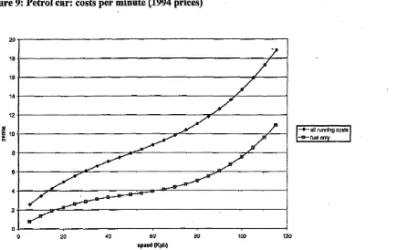
those related to the cost of the employee (which is what we want), and those relating to vehicle operating cost. In making comparisons of different results, it is important to keep this in mind

In the latest TEN, Working Values of T i in pence per hour are provided for a number of "driver" categories: these are in average 1998 values and prices, based on average wage rates from the 1998 New Earnings Survey, factored up by a factor of 1.241 to reflect overheads, and are thus in line with the theoretical discussion above.

Converting to end-1994 values, for comparison with AHCG results, we allow for a growth in real GDP per head of 8.9% and 12.3% inflation, giving an overall deflator of 1.223. We use the "perceived" values from the TEN table:

The question of relevance is then whether the AHCG empirical data and analysis has something to contribute to the discussion of working time values. In addition to the topic of "business" travellers to which we return below, SP surveys were canied out for Coach & Bus Operators, and Freight Operators. We discuss these in turn.

Category Car driver

LGV occupant (driver or passenger) OGV occupant

PSV driver

3.2 Coaches and Buses

TEN VTTS converted to end 1994 plmin 23.8

10.0 10.0 9.1

For Coach and Bus Operators, AHCG sampled 10 Scheduled Bus Operators, 9 Scheduled Coach Operators, and 28 Chartered Coach Operators: the aim was to contact the "Key Decision Maker regarding routeing"

-

specifically not the driver himself. In addition to collecting considerable information about the mode of operation, fleet composition etc., the respondent was presented with 2 SP experiments, one relating to "within-route" options where 'total transport time" and "total transport costs" were traded, along with two other attributes relating to information and unexpected delay, and the other a choice between an untolled and a tolled route, with transport costs otherwise constant, but transport time varying and, on the tolled route only, some information provision.

From the interview transcripts provided by AHCG it is clear that the "Total Transport Costs" are meant to represent the cost of operating the service for a one-way journey, specifically "includiig drivers wages, fuel etc." On this basis, it is far from clear what the trade-off between "total transport time" and "total transport costs" implies, since all time-related costs should have been converted into money terms.

Trunk Road Charters" (p 235). It appears that the Charter segment has been split on the basis of response to the 'type of road used most extensively" for the service in question, with approximately 40% assigned to Trunk roads. Bearing in mind that the estimations have not been corrected for repeated observations, none of these results carries a high level of statistical significance.

In the case of Experiment 2, respondents were asked to identify an alternative route and to estimate the total cost (including wages) and time: these values are then used as the basis for the variations in the SP variables. Once again it is hard to interpret the trade-off actually being made: for example, the costs are only varied in respect of the toll, but the times on both routes vary independently, without any impact on wage costs. On grounds of practicality, Experiment 2 was not given to Scheduled Bus operators.

Two models are presented, one which excludes the subset who always rejected the tolled route (possible policy response bias): in terms of VTTS, the differences are small, and using the results which exclude the subset noted above, the values are about 58 plmin for Scheduled Coaches, 24 plmin for "Motorway Charters", and 20 plmin for Trunk Road Charters. Only in the case of Motorway Charters is a high level of significance reported.

In drawing conclusions,

AHCG

note the following:

For coach, the study was designed to offer a new insight into factors affecting operators' valuations of travel time by interviewing the operators themselves, differing from the COBA approach which looked instead at the VOTs for driver and passengers. As with freight, the direct approach to the operators, as taken in this survey, has been judged to yield the appropriate VOTs for forecasting: for evaluation, however, we would recommend retaining the COBA approach, rather than adding on passengers utility change from the time savings/gains to the operator's VOT. This difference is due to the expectation that the operator's VOT will include the expected fare increasddecrease that could be charged for a faster/slower service, which will in turn be some fraction of the passengers' utility change from the time savingdoss. Simply adding the two would then result in double counting. [p

2951

In our judgment, it is highly unlikely that in responding to the SP tasks, the operators have been able to take into account the assumed elasticity of demand to travel time variations and the potential for recouping this through the farebox! More generally, we have concerns about the whole context of the tradeoffs. Assuming that they are intended to represent both wage costs and operating costs, we might expect the element for operating costs, based on the formula in TEN, to contribute about 50pImin for coach (assuming an average speed of 80 kph) and around 2lplmin for Scheduled Bus (assuming a running speed of 20 kph). Note that these are in 1998 values, so for comparison might be reduced by 20%.

3.3 Commercial Vehicles

Turning now to the corresponding freight surveys, essentially similar methodology was used. AHCG sampled 165 Hauliers (of whom 118 were classified as HGV) and 105 "Own Account" Operators (of whom 48 were classified as HGV). Both the identification of the "Key Decision Maker" and the presentation of the SP experiments followed the lines of the Coach surveys.

In this case the interview transcripts make it clear that the "Transport Costs" are meant to represent the "typical cost for a shipment", excluding loading, unloading and handling costs.

It appears that this should therefore also include driver's wages, fuel etc. Once again, therefore, it is far from clear what the tradeoff between "total transport time" and "total transport costs" implies.

For the fust experiment, AHCG report "VOTs for the Hire and Reward segments are about 45plmin and for the Own Account segments about 35p/min, with almost no differences between LGV and HGV" (p 232). The level of statistical significance is reasonable. We have some reservations about the credibility of the timelcost trade-offs offered in this experiment since we think that routes with big time/cost trade offs are quite rare in the

UK.

(Portsmouth and Southampton to various destinations is one example).

The second experiment involves choosing a toll to use the quicker (current) route against a slower free alternative. This is believable, but causes a different problem, an anti-toll bias. Values are around 20plmin except HGV own account which is 33pImin. However, 25 per cent of the sample refused to trade time for money and the results therefore depend on the plausibility of the responses of this group. The models excluding the subset who always rejected the tolled route produce generally similar VoTs, except for HGV Own Account, where the value rises to 59 plmin.

As with the coach SP, respondents were asked to idenufy an alternative route and to estimate the total cost (including wages) and time: these values are then used as the basis for the variations in the SP variables. Once again it is hard to interpret the tradeoff actually being made: for example, the costs are only varied in respect of the toll, but the times on both routes vary independently, without any impact on wage costs.

In contrast to the Coach surveys, the two experiments lead to results which are significantly different. Apart from the HGV Own Account group, which are more or less the same between the two experiments, but increase strongly (as noted) when the "non-traders" &removed, the experiment 2 values tend to be about half the experiment 1 values. This might be expected on the basis of

a

toll response bias, but it was not found with the Coach SP.

As with the coach surveys, we have concerns about the whole context of the tradeoffs. Assuming that they are intended to represent both wage costs and operating costs, we might expect (assuming an average speed of 50 Kph) to add about 9 plmin for LGV operating costs and between 20 (OGV1) and 35 (OGV2) plmin for HGVs: these are in 1998 values, so for comparison might be reduced by 20%.

In line with the arguments used elsewhere in this report, AHCG favour the use of results which are not based on tolls. Accordingly, they recommend the use of the values from Experiment 1 quoted above. Other work, some of it recent work for the Highways Agency, is reported in the working paper. However much of this work is aiming at the value of reducing unexpected delays rather than the value of a pure 'anticipated' time saving. It is difficult to make secure deductions about the latter from evidence on the former.

Expt 1 TEN adjusted

Expt 2 (excl non-traders)

While the Experiment 2 LGV figures are consistent with the TEN values, all the AHCG Experiment 1 figures apart from the HGV Own Account are well in excess of the "wage rate plus" values. The lack of difference between LGV and HGV is difficult to accept, given the much higher operating costs for the latter.

It is worth noting that deriving reliable values of time savings for freight transport from willingness to pay based approaches is a notoriously difficult task.

LGVHgrR 43.5

17.5 15.1

the industry is heterogeneous and there is a problem of finding a suitable sampling frame from which to ensure a representative sample is taken;

the respondent, who might be a transport manager, is unlikely to have a comprehensive perspective of the impact of time savings on the overall value to the logistics chain; this is particularly true of respondents in the Hire and Reward sector

there are difficulties in representing designs and choices which are relevant and credible to the respondents; some researchers have sought to overcome this problem by using adaptive SP methods

ideally we would like to separate out the value of a unit time saving or loss which is fully understood and anticipated in advance by the firm (such as a decision to impose a legal

maximum speed limit of 90 kph) from the value of changes in unexpected delays (policy actions which reduce travel time variability). In practical SP experiments, this can be problematic.

On balance, we do not think the empirical evidence is sufficiently strong to warrant moving away from the traditional COBAITEN approach to valuing "pure" time savings. We note that the TEN currently assumes a vehicle occupancy of unity for commercial vehicles. We recommend a small study be undertaken to establish the acceptability of this assumption.

LGVOA 35.5

17.5 17.7

3.4 ccBriefcase" Travellers

For these people it is clearly an empirical question whether r and p in the Hensher formula are sufficiently different from zero to be worth calculating. To date, the UK authorities have not been convinced of this. A particular problem is how to pose the survey questions to obtain reliable answers.

HGVHBrR 47.1 26.7-39.2 20.5

In an earlier discussion, Fowkes et a1 (1986a) made a number of observations, based on surveys of business travellers intercepted travelling on East Coast Main L i e trains, or via employers in Newcastle.

HGVOA 35.5 26.7-39.2 59.3

average indifferent between travelling (working or not) and working in the office. This hardly seems satisfactory from a theoretical point of view, but might not be far wrong on average.

For p, the proportion of travel time savings which is at the expense of work done whilst travelling, Fowkes et al felt that those who do work while travelling generally work for a sufficiently short time that realistic travel time savings would have no impact. So while the proportion of

total

travel time spent working has empirically been found to be greater than zero for groups of business travellers, giving the value of p used by Hensher, Fowkes et al felt that this should be called p*, with true p lying between zero and p*. Estimated values of p* ranged from 0.03 for car to 0.21 for rail.

For q, Fowkes et a1 followed previous practice by asking how long was worked on a particular trip, and how long that work would have taken in the office. They state that, due to the expected overreporting of work done, it is to be expected that q will be biased upwards, but really it is a second bias effect affecting q that is the problem. It is not that a lot of work was done while travelling, it is more the claim that it was no less productive per minute as work in the office. For car the reported average value of q was above unity, and it is hard not to imagine that as an overestimate. For air the average was 0.98 and for rail 0.95.

For r, Fowkes et al rejected the use of the proportion of total travel time which occurs in leisure time. Firstly it was felt that for day trips starting and ending at home, where there is sufficient work to be done at the destination, travel time savings are likely to result in more time spent at the destination, rather than a later start from home or an earlier arrival back (though this is complicated by public transport schedules). Secondly, business travellers may be able to substitute travel out of normal work hours for work time on another day. Accordingly, Hensher's value was denoted r*, and the true value of r taken to lie between zero and r*. Values of r* found varied from 0.32 for car to 0.42 for rail and air.

All this implies that the Hensher formula will be some weighted average of MP and the private VoT,

VL.

Since VLcMP, the formula will in general give lower values

than

the wage rate approach. On plausible assumptions, VTTS for car might be 80-90 per cent of the wage rate, for rail and air perhaps 65-75 per cent. However, it seems that employers' willingness to pay for time savings is greater than the gross wage rate (perhaps MPF

>O,

or additional time at the destination is particularly valuable) so that the final VTTS for business travel is not very different from the gross wage (Fowkes et al, 1986).

Having discussed the formula in general, now we consider how

AHGG

implemented it.

In order to estimate values corresponding to the Fowkes et a1 parameters (1-r*), p* and q,

AHCG

asked car travellers the following questions:

Q20 Suppose that the business trip that you were making had taken 15 minutes longer as a result of congestion on the roads. Would that extra time have been paid by your employer, or would it have come mostly out of your own time [or a combination of both]?

Q21 Did you use any of the time during that trip to do work which you otherwise would have done elsewhere; for example preparing for a meeting, conversations on a portable telephone, etc?

If

so, about how much time?

Given that total travel time is known, this question allows us to estimate p*, the proportion of travel time spent working. AHCG found that 22.2% of respondents did do some work, the average proportion for these people being 0.195. Hence p* = 0.222 (0.195) = 0.043. The Fowkes et a1 car value for p*, was 0.033, but this applied to long distance only, in which case the AHCG value rises to 0.052. Perhaps this reflects the increasing use of mobile phones, laptops etc., or perhaps 'mental' preparation was included thereby changing the defmition compared to the earlier study.

Q22 Approximately how long would that same work have taken you ifyou had done it at

your office or at your home?

This question is clearly an attempt at findimg q, the relative productivity of work done while travelling compared to in the office. The mention of 'or at your home' is a complication however, since it is quite possible to imagine the office being the most productive environment per minute work, followed by 'in car', with 'at home' being the least productive. In any event, values found were close to unity, averaging 1.02. Ignoring journeys of less than 30 minute reduces that to 1.01. Fowkes et al found q values of 0.96 and 1.07 in their two samples of car business travellers, averaging 1.01, thereby agreeing (rather by fluke) with the AHCG long distance car figure. The agreed figure is, however contrary to the expectation that q is significantly less than one. How to proceed from this point is not clear. The simplest approach is to say that there are no grounds for taking q to be any value other than 1.00. Another approach has been to replace q values above unity by unity, on grounds of plausibility, and then recompute the average. Attempts to do this can lead to big changes in q, though the effect on VTTS is not large.

All this suggests that the true value of pq is very little different from zero, and the main attention therefore turns tor.

The AHCG study gives the value of travel time savings on employers' business as

Compared to the "Hensher" equation, MPF is dropped, and it is assumed that

W

-

the "employee value" in the "Hensher" equation given earlier

-

can be taken as the Business Traveller's (private) VTTS. This implies that in responding to the SP tradeoff questions, Business travellers take into account whether time increases or reductions will be transferred tolfrom leisure or work. According to Gunn (2002), 'Exploratory work was done to check for biases in cases where employees might pay, both by stressing a non-reimbursement conditionZ prior to asking for the trade-off, and by checking for the impact of any re-imbursement on the derived values."

In the case of those who answered that time increases would come out of their own time to Question 20 above, ie r* = 1, we may assume that the expressed estimate of VP is equivalent to VL. The question then is: will those who give values of r* = 0 provide estimates of

VP

equivalent to VW (with an intermediate value for those who give r* = 0.5)? We find this a priori most unlikely, particularly in the light of the reimbursement condition. If Business respondents are encouraged to think that cost changes whether positive or negative will be borne by them personally, are they not likely to think the same for time changes? Note also

he instructions preceding the first Stated Preference experiment were: "If you did not actually pay for the journey yourself, please assume that you would receive a fixed amount of reimbursement equal

that Question 20 relates to time increases being paid for, rather than whether they would shorten the amount of time spent working. Hence, we incline towards the view that the SP is likely to provide a value of

VL,

irrespective of the value of r*

We note that the AHCG version of the equation is also used in Algers et a1 (1995), but with a slightly different interpretation:

"In this study, the value of time to the employee was not differentiated depending on whether the time saved would be spent at work or on leisure, and it was thus implicitly assumed that the private VOT (VP) is the same in both cases, or that VW equals

VL."

Setting VW equal to VL implies that the marginal utility to the employee of time in work is assessed equal to that spent in leisure. We feel that this is incorrect ; for most business travellers, VW cannot be assumed to equal VL, since travellers will not be indifferent between spending time working and leisure time. Although we understand that the equivalence was assumed because it was unclear whether the saved time would be transferred to leisure or working, we think it is more plausible to assume that

V W ,

as defined, equals zero.

At face value, therefore, allowing for the ''near zero" value of pq, this might suggest the simpler formula:

VTTS = (1-r).MP

+

r.VL

On our interpretation, a value of VL, the private value of time for Business travellers is available from AHCG, and for those travelling on their "own time and money" is reported as

6.7 p/min3. In order to calculate the final outcome, AHCG required an average wage rate for their business sample, which they estimated as 30.9 plmin. Their explanation of this is as follows (p 254):

This assumes that the annual household income (taken as the midpoint for the survey category) is divided by 1800 hours per year, and then adjusted for the number of workers in the household (because the business traveller generally earns the bulk of the household income, 2 workers is assumed to equal 1.5 equivalent 'work years' and 3 or more workers to equal 2.0 'work years). Finally, a factor of 1.4 is applied to account for extra wage-related costs.

There are several assumptions involved here, which taken together make the final figure highly unreliable. Our overall view is that the Hensher formula approach is data hungry, and that none of the various parameters r, p and q are at all easy to estimate with confidence. AHCG have made a fair attempt, but their basis for imputing the MP values is weak. Therefore we cannot recommend adoption of the approach taken and values derived in the AHCG report.

There remains the question of what should be done about the possibility that business travel time savings may be used for leisure purposes

(d).

There would appear to be two significant groups of interest: those who can take time off in lieu for travel time outside of normal working hours, and those who accept some out of hours travel as a condition of the job.

In the former case, any time saved for travel time reductions will either result in additional time spent at work directly, or indirectly due to less time taken off in lieu. Such arrangements

may only work imperfectly, but we feel that the gain to the employers will be near enough the gross wage rate.

In the latter case,

if

we assume that the labour market is working correctly, then it must be the case that remuneration packages for this group reflect that there is a significant amount of out of hours travel which cannot be set against time taken off in lieu. If there are travel time savings resulting in an hour saved, then some of that may result in extra work completed and some may reduce the amount of travel undertaken out of hours. To analyse this, it will suffice to consider the two extreme cases: all in work hours, all outside work hours.

When all travel is during working hours, it is clear that the benefit to the employer is most simply taken to be equal to the gross wage rate. Note that, particularly in the context of long distance day trips, having three hours at the destination instead of two could be especially valuable, e.g. three productive hours in a ten hour working day instead of two. In the second case, where the time at destination is held constant but the journey starts later and/or ends later, the employee receives the immediate benefit. For day hips there can be a considerable benefit, since extra time in bed in the early morning is paaicularly highly valued (according to the Fowkes et a1 sample), and presumably time saved late in the day may also be highly valued. In this context, we are attracted by a flexible wage assumption rather than the rigid wage assumption underpinning the Hensher formula. That is, given these improvements in the conditions of work, it is reasonable to assume that profit maximising employers will wish to take them into account when deciding aspects of the remuneration package.

Our

view is that the simplest assumption to make is that if employee A is spending one hour less on company duties, the employer will be able to pay that employee one hour's wage less, all else equal.

It has been suggested in discussion (Gunn (2002) that this requires an ability to forecast the way in which wage rates would alter to reflect changes in the onerousness of travel. However, the argument above does not relate to wage rates as such, but to the total remuneration. Salaries can fall if working hours are reduced without any implication for the wage rate.

To summarise our conclusions for the valuation of time savings for employers' business hips:

for professional drivers, there is a strong justification in principle for retaining the 'cost saving' approach;

there is a great deal of uncertainty about the 'true' values of the parameters in the Hensher model such as r, q and p, in spite of the effort put into devising suitable questions;

there is also doubt, in any case, about whether changes in the onerous nature of working conditions, including travel time on employers' business, are not anyway in the medium term reflected in the total remuneration;

given these uncertainties, and given that alternative assumptions give results either side of the Department's current value, we see no strong case for abandoning the cost saving approach for valuing savings in travel time for briefcase travellers;

4. SIZE AND SIGN OF TIME SAVINGS

The conventional

UK

approach has been to use standard values per minute regardless of the sign and size of the saving. This has attracted criticism from those who argue that small time savings should be valued at a lower unit value than standard (Welch and Williams, 1997). This is an important practical issue for road appraisal, since if "small" is defined as, say, less than 5 minutes, most time savings on most schemes would fall in that category.

Anticipating issues of practicality, it must be conceded that any attempt to introduce sign and size variation (more generally, non-linearity with respect to time changes) into the appraisal process is fraught with difficulties, for reasons which have been well rehearsed, relating to essential concepts such as additivity and reversibiiity within the Cost Benefit appraisal. Nonetheless, this in itself is no reason not to attempt to see whether such variation exists.

The AHCG study set out to examine this fully, and found that, "For any level of variation around the original journey time, gains (savings) are valued less than losses. For non-work related journeys, a time saving of five minutes has negligible value". However, AHCG did not recommend that values for appraisal should be differentiated by size and sign. We have reanalysed the AHCG data to see whether further light can be shed on the two findings above.

4.1 Sign of Time Savings

From first principles, one might expect an indifference map of the form shown in Figure 1. Starting from the origin, in quadrant 4 every unit cost increase requires increasing amounts of time saving to justify it as the money budget constraint binds tighter. In quadrant 2, every unit time increase requires increasing amounts of money to compensate as the time constraint binds tighter. While the expected curvature is clear, the scale of the diagram is unspecified. A reasonable conjecture is that the curves might approach linearity for small changes in cost and time, though empirical evidence could refute this.

Note that the theoretical form of the indifference curve requires the sign of the second

a2uk

derivative

-

to be non-positive, and this is incompatible with any implications that small at

-.

time savings are valued at a lower unit rate. Nonetheless, the theoretical form, of course, assumes that (utility maximising) behaviour is reassessed in the light of any changes in travel conditions, and in the short term this may not be the case.

The main AHCG stated preference experiment (see Appendix B) offered a series of pairwise comparisons where the two options were characterised solely in terms of changes in time and money. These involved the following types of trade-off:

A choice between an option which was slower than the current journey and an option which was more expensive, other things equal (quadrant 1).

A choice between an option reflecting the current situation and an option which was slower but cheaper than the current situation (quadrant 2).

A choice between an option which was quicker than the current journey and one which was cheaper, other things equal (quadrant 3).

The options were specified as changes to the current situation. Across all the different designs, nine levels of time variation were used: time savings and losses of 5, 10, 15 and 20

minutes and a 3 minute time saving.

Figure 1

-

The standard indifference map

In what follows we provide an abbreviated description of our investigations. More detail is available in ITS Working Paper

WP561,

and for most of the models mentioned here, details of the coefficients and model fit are given in Appendix E of this Report.

We began by reproducing the basic model results [Model 4-11 set out on page 162 of AHCG's final report. This model can be written:

where: i relates to an individual journey

k relates to a design "treatment"

-

ie a single SP painvise choice j relates to pairwise option A or B within treatment k

As is standard in Discrete Choice analysis, we work in terms of a "utility formulation". Since increased cost and time convey disutility, we expect the coefficients to be negative. In its simplest linear form, as given here, utility is directly compatible with "generalised cost", except that for the latter the coefficients are set to be positive, so that it is in fact a measure of disutility, The "value of time" is calculated straightforwardly as the ratio of the marginal utilities of time and cost, thus in this linear case, VTTS =

P/Pc.

In AHCG the model is estimated with a tree structure and the cost coefficient constrained to equal 1. This allows the value of time and the associated t-statistic to be a direct output of the model. We have dropped the tree structure and coefficients are freely estimated for time and cost changes. All our models have been estimated using GAUSS software (Aptech Systems, Inc, Maple Valley, WA 1996).

Table 1: M1 Base Models [=

AHCG

Model

4-11

All t-statistics are given relative to zero. As is the case with AHCG, we have not in this Report carried out any adjustment on the standard errors to allow for the "repeated measurements" problem (though AHCG report some later work using Jackknife techniques). Thus we should have some caution in interpreting the t-statistics and possibly the log- likelihood ratios as well: we can expect the level of significance to be generally somewhat overstated.

Investigations of this model (MI) suggested that the data would support a non-linear utility specification implying variation in VTTS with the sign and size of the time change. There are various ways in which non-linearity could be reflected. The basic AHCG approach was to allow for different coefficients on time and cost according to the sign of At and Ac. In fact, AHCG do not report the results of such a model, but move on immediately from the basic model (Ml) to one which includes other terms as well (AHCG Model 4-2), chiefly due to size effects. However, we have estimated this model ( ~ 5 3 . Because each combination of positive and negative values of At and Ac implies a different "quadrant", it is possible to calculate the implied variation in

VTTS

for each quadrant, and these are reported in Table 2 for each of the three journey purposes. It can be seen that the values obtained in quadrants 1 and 3 are

broadly similar; however in quadrants 2 and 4 they are spectacularly different (ratio 4.6,7.7, 8.4 for the three purposes).

Other -0.0545 (15.31) -0.0122 (25.36) 4.5 -0.632679 8038 Time Cost

value of time (plmin) Average

LL

No. Obs

Table 2: Re-Analysis of the

AHCG

Data (1994 pence per minute)

While the comparison between quadrants 2 and 4 appears to support the AHCG conclusion that losses are valued significantly more highly than gains, we have doubts about the validity of this interpretation. In the AHCG survey design, respondents were fust asked to give details of the journey being made at the time of recruitment. They were then offered various timelcost choices and asked to state their preferences. For the offers which fall in quadrants 1 and 3, the respondent's journey is used to frame the choices offered, but is not directly included in the set of choices offered. However, for the offers which fall in quadrants 2 and 4,respondents were offered a choice between their existing time and cost and a faster more expensive alternative( quadrant 4) or a slower cheaper journey (quadrant 2). Previous exploratory analysis (Bates, 1999) had indicated that AHCG's fmdings with respect to sign

Business

-0.0780 (26.30) -0.0075 (24.51)

10.4 -0.649687

9557

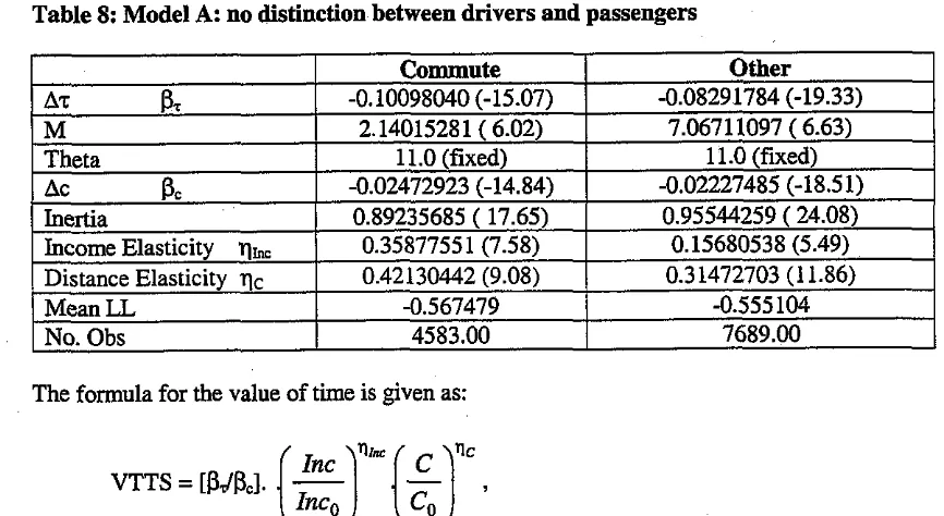
The details of the model are given in Table 8 of ITS WP.561

could be explained by the presence of an "inertia" effect. In this context, inertia is a systematic preference for the current situation, and in the

AHCG

design this is confined to choices relating to quadrants 2 and 4. If there is an inertia effect of this form, we would expect the values of time in quadrant 2 to be inflated since respondents will be less prepared to suffer a time loss in return for a cost saving. In quadrant 4, the inertia effect would lead to a lower willingness to pay than otherwise.

It is convenient to refer to the dummy variable which signifies that an option (in quadrants 2 or 4) coincides with the current joumey as "inertia". The presence of true inertia in transport behaviour is well-attested: however, the explanation has usually been advanced in terms of the cost of acquiring information about altematives, or, slightly differently, the uncertainty surrounding the performance of the alternative. In principle, neither of these reasons should apply to SP where the information about the altematives is provided directly and without qualifications (though there remains the possibility that the respondent may not believe it!). In addition, the altematives presented have no inherent characteristics (as might be the case, for example, with different modes), and therefore there is no reason to postulate any "brand loyalty". In this case, therefore, it is more difficult to conceive that a true inertia effect is present.

However, for an SP respondent, choosing the current situation in a choice context may be a safe option, and one which avoids having to make a careful assessment. There is also the possibility &at people may tend to believe m&e that they will get the costs than that they will get thi benefits! If a respondent is adequately satisfied with his current journey, he can avoid the effort of assessing the tradeoffs in Quadrants 2 and 4 by selecting the current joumey. Taken at face value, this will therefore in itself imply low values of time for time savings and high values of time for time losses, unless the possibility is allowed for. In the case of tradeoffs in quadrants 1

and 3, there is no obvious way in which one of the options can be regarded as "special".

If the effect in Model

(M5)

relates genuinely to the sign of the cost and time changes, then the same results should be obtained whether we confine the data to quadrants 1 and 3, on the one hand, or quadrants 2 and 4, on the other. We therefore estimate a partitioned version of Model

(M5)

for these two subsets of the data. The results were striking: confining the data to quadrants 1 and 3 produced no evidence of an effect due to sign. Moreover, when an inertia term was introduced into the estimated utility functions for the data in quadrants 2 and 4, it was found to be highly significant and no significant differences between the values of gains and losses remained. On this basis we pooled the data again, but included the inertia term for all observations relating to quadrants 2 and 4. We referto the corresponding model as (Mll).

As Table 3 shows, the overall fit? of the model with inertia (Mll) is far better than that which differentiates the values by sign (M5), despite the former containing one less parameter. We therefore do not accept the

AHCG

conclusion that the VTTS should be differentiated by sign.

Table 3: Comparison of Model Fit

(LL

per observation)

More details of the models are given in ITS WP561

[image:23.541.74.499.587.721.2]

We note that an inertia effect was also apparent in the findimgs of Dillen and Algers (1998) who used a similar design. We have also conducted some analysis on the Tyne crossing route choice SP data set collected in the first British national value of time study (MVA et al., 1987) and one collected in the

AHCG

study. In neither case is there evidence to support the VTTS varying by sign.

Hence, as set out in WPS61, we do not believe that the

AHCG

conclusions on variation by sign are safe, and within the likely range of variation, we do not believe that there is any empirical basis for distinguishing gains or losses.

4.2 Size of Time Change

Having introduced inertia terms to account for sign effects, we conducted further re-analysis of the

AHCG

data to examine the size effect. There are different ways in which this can be demonstrated, but we are in no doubt at all from the resulting models that, as

AHCG

found, the unit values of 'small' time changes come out very different from 'large'.

In investigating what the data tells us about small time changes, it will be sensible to correct, as far as possible, for the journey covariates. This is particularly the case since the smaller changes (3 and S minutes) tend to be presented in relation to the shorter journeys (See Appendix B on the design). It is convenient for the analysis of small time changes if we can confine the effect of the journey covariates to the cost coefficient: in fact, this turns out to be the preferred model specification (Model 6d).

We began by creating dummy variables for each time change, thus allowing us to estimate the utility for each of the values At = (-20, -15, -10, -5, -3, +S, +lo, +IS, +20). Note that this is close to the final specification adopted by

AHCG

(ignoring the inertia effects) except that they dropped the term corresponding with At = -3, thus presumably forcing it to have a zero valuation.

The findings (Model ~ 7 1 ~ ) are given in Table 4. For changes of 10 minutes or greater, values of time of around 5 pence per minute are found for non-work purposes. For changes of less than 10 minutes, the values are found to be close to zero, or even negative. Although our model specification is different, these findings are not essentially in disagreement with those reported by

AHCG.

Table 4: Values of T i e by Size of Time Change (plmin)

"ore details of the model estimation are given in ITS

WP

561

A number of tests were conducted to attempt to identify the likely causes of this pattern of results. On the face of it, it is possible to hypothesize a number of reasons as to why these results are occurring: they could be related to

problems with the analysis problems with the design

problems in responding to the SP tasks

The implied negative values of time are, taken at face value, simply illogical. However, it is critical to note that the design does not offer respondents any opportunity to display a negative value of time

-

e.g. by choosing a time increase rather than a cost decrease. Hence, if negative values are derived, this would seem to be an outcome of the model specification, and need not imply that the data is illogical. To see why we are obtaining these model results, we need to go back to the data.

In practice, we do not expect all respondents to evince the same value of time, and there will be a distribution. The proportion choosing the cost saving should rise as the cost saving increases. We therefore examined all the tradeoffs in Quadrants 1 and 3. Apart from minor variations, the data for each purpose confirmed that:

for a given value of At, the propensity to choose the lower cost option increased as the cost difference increased; and

for a given value of Ac, the propensity to choose the lower cost option decreased as the time difference increased

This is precisely what one would require on grounds of general rationality.

In a prior review of the

AHCG

study, Fowkes and Wardman (1999) had raised some concerns about the adequacy of the SP design. We therefore subjected the designs to testing using synthetic data and found it to be able to recover a large range of values of time remarkably well. We are confident that the results being obtained are not artefacts of the design.

We also used the mixed logit model of Revelt and Train (1998) to examine random taste variation but although the specification of a lognormal distribution for the time coefficient removed the negative values of time, the broad pattern of results for small time changes remained.

The phenomenon of apparent negative values is discussed at length in Working Paper 561. The explanation is technical and concerns the assumptions of the logit model in situations where large proportions of respondents refuse to trade time for money in the SP at any of the rates offered. This explanation suggests that the apparent negative values of time are not a true feature of the data, and that a model form is required which does not allow the value of time to go negative.

The most consistent model which we could develop to explain the data involved a "tapering" function

(MS),

whereby time changes offered in the SP exercise below a "threshold" of 11 minutes were progressively reduced (as if respondents perceived that the actual time change would be smaller). In place of including the presented time change At in the model specification, we substituted a modified value AT, where7:

AT = Sign (At)

*

{ ]At]

.

[ lAtl2 €I]

+

€I.( IAt]/€I)". [ ]At1

<

81

1

where 0 is the threshold value (estimated at 11 minutes), and m

>

1 an estimated "tapering" parameter. The rate of "tapering" was highest for Other purpose travel, and lowest for Business travel. Note that when m = 1, AT = At. The results for this model are given in Table 5:

Table 5:

MS

models with "perceived" time coefficient (8

=

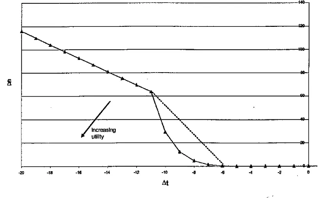
11)

If we transform to indifference curves, we obtain the pattern shown in Figure 2. While these curves now respect the theoretical condition on the first derivatives, thus avoiding implications of negative values of time, they clearly do not respect the conditions on the second derivatives. It should be noted that the symmetry results from the constraints imposed by the model form, where there is assumed to be no variation by sign.

In Table 6 we set out the statistics for overall model fit as relates to the size effect. Although our preferred model (Ma) is not the best fit to the data, it is considerably more parsimonious in terms of parameters and avoids illogical negative values of time, which we have shown are inconsistent with the data.

[image:27.541.82.476.49.259.2]

Figure 2: Indifference Curves with Perception Effect

1-

B U S ~ ~ ~ S S

-

Camrnute +Other

I

Although the data strongly indicates that a lower unit utility'attaches to small time changes (whether positive or negative), we feel it would be unwise to take these results at face value. In the first place, the results are inconsistent with the theoretical expectations on the shape of the indifference curve, at least when allowance is made for adjustments beyond the immediate short term. Moreover, it implies extremely high marginal values of time as the threshold of 11 minutes is approached.

[image:28.577.83.421.88.291.2]

Figure 3: Illwstration using Implied Indifference Curves

The inconsistency is associated with a violation of the convexity of preferences: according to this, if the average traveller is indifferent between say a time saving of 6 minutes with zero cost and a time saving of 11 minutes costing 64p, then we should be able to find some intermediate point along the dashed line joining these two points (e.g. a saving of.8.5 minutes costing 32p) which would make him at least as well off. In fact, the indifference curve lies below the dashed line, suggesting that he would be worse off at any intermediate point along the dashed line.

Effectively, the data is telling us that for time changes between 0 and 6 minutes, the value of time is more or less zero, for a further change of 5 minutes the marginal value of time is on average 12.8 plmin, and thereafter it reverts to about 5 plmin.

In general, the following kinds of explanation may be considered:

(a) The data reflects real perception and preferences. People are willing to trade at a lower rate for small changes than for large. This would lead to a recommendation (at least for modelling) of lower unit values for 5 mins or less than for 10 (or, perhaps, 11) mins or more.

(b)

The data relating to small time changes as presented in SP is unreliable. People's

perception of the problem is defective, there is a failure of belief, and they refuse to trade at a plausible rate. This may be because they believe such time savings would not actually come to pass or are minor alongside day-to-day variation in car journey times.

(c) Alternatively, people may take the SP offer at face value, but perceive themselves