4 Psycholinguistics
In psycholinguistic experiments, research factors such as word frequency, syntactic
construction, or linguistic context are manipulated in a set of materials and then participants provide responses that can be scored on a continuous scale - such as reaction time, preference, or accuracy. The gold standard approach to the quantitative analysis of this type of data
(continuous response measure, factorial experimental conditions) testing hypotheses about experimental factors is the analysis of variance (ANOVA).
Of course psycholinguistics is not the only subdiscipline of lingusitics for which ANOVA is relevant. In fact, the structure of this book around particular subdisciplines of linguistics is a little artificial because most of the techniques find application in most of the subdisciplines. Nonetheless, multifactor experiments with analysis of variance hypothesis testing is the primary methodology in psycholinguistics.
We are cycling around the two key ideas of chapter 2 that I called “patterns” and “tests”. In that chapter I introduced hypothesis testing and correlation. That was orbit number one. In chapter 3 we went further into the t test, emphasizing that the t test is a comparison (a ratio) of two
estimates of variability, and we spent some time discussing how to find the right estimates of variation for use in the t ratio. Then we dipped into the correlation matrix to see how to find data patterns using regression and principal components analysis. That was orbit number two. In this chapter we are going to stay with hypothesis testing all the way - keeping our focus on analysis of variance. Then in the following chapter on sociolinguistics we will stay in pattern discovery for a chapter. The interesting thing is that by the end of all this we will have blurred the line between hypothesis testing and pattern analysis showing how the same basic statistical tools can be used in both, concluding that the difference lies primarily in your approach to research rather than in the quantitative methods you use.
4.1 Analysis of Variance: One factor, more than two levels.
With only two levels of a factor (for instance sex is male or female) we can measure an
experimental effect with a t test. However, as soon as we go from two to three levels the t test is not available and we move to analysis of variance.
progressed then one might conclude that the priming effect has more to do with the listener’s strategy in the experiment than with a necessary benefit (or impediment) of phonological overlap.
In a phonological priming study the listener hears a prime word, to which no response is given, and then a target word, which does recieve a response. The response measured by Pitt and Shoaf was “shadowing time” - that is how long in milliseconds it took the listener to begin to repeat the target word. For example, in a 3-phoneme overlap trial the listener would hear the prime “stain” and then the target “stage” and then respond by saying “stage”. In a 0-phoneme overlap trial the prime might be “wish” and the target “brain”. Shadowing time was measured from the onset of the target to the onset of the listener’s production of the target. Pitt and Shoaf had a large number of listeners in the study (96) and were able to compare the first occurance of a
3-phoneme overlap trial (after a long initial run of trials with zero overlap) with the last 3-3-phoneme overlap at the end of the experiment. We’ll take advantage of their large subject pool to first explore Analysis of Variance with data sets that have a single observation per listener - reaction time from a single trial.
The simple models that we are starting with don’t work for most psycholinguistics experiments because psycholinguists almost always use repeated measures (see section 4.3), so I’m using simple models to test subsets of the Pitt & Shoaf data where we have only a single observation per listener. Keeping our analysis for now confined to a single data point per person allows us to avoid the complications that arise when we examine data that involve multiple observations per person. Another characteristic of these initial datasets that makes it possible to use classical ANOVA is that we have an equal number of measurements in each cell.
---A short note about models. The analysis of variance is a test of a statistical model of the data. “Model” is a pretty popular term and is used to mean different things in different research
Here’s a simple statistical model of the sort we are considering in this section:
€
x
ij
=
µ +
τ
i
+
ε
ij
“treatments” modelThis statement says that we can describe an observed value xij (a response time, or accuracy measure, for example) as made up of three components - the over all mean µ, the average effect of the ith treatment effect (τi), and a random error component (
εij
) that is unique to this particularobservation j of treatment i. This statistical model assumes that the treatment effects (τi) which
are the experimental factors or conditions in a psycholinguistic experiment are different from each other. When we find that the treatment effects are different from each other (see below) we can report that there was “a main effect of factor τ” (we’ll get to interaction effects later). This
means that the best fitting statistical model includes this factor. The ANOVA compares the model with τ against the null hypothesis which says that we can just as accurately describe the
data with a “no treatments” model.
€
x
ij
=
µ
+
ε
ij
“no treatments” modelBut, “describe the data” is the right way to characterize what these statistical models do. An explanatory account of why the treatment affects the response requires a theory that specifies the mechanism - the statistical model is good for testing whether there is any effect to be explained but does not provide the explanation.
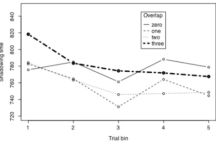
---The analyses that I will describe in this section and in section 4.2 assumes that each observation in the data set is independent from the others. I selected data from Pitt & Shoaf’s raw data files so that this would be true by following the sampling plan shown schematically in table 4.1. Listener S1 provides a data point (x1) in the no overlap, early position condition, listener S2 provides a data point in the no overlap, mid position cell, and so on. With this sampling plan we know that observation x1 is independent of all of the other observations as assumed by the analysis of variance. It was possible to follow this data sampling plan because Pitt & Shoaf tested 96 listeners (16 in each column of table 4.1) and this is a large enough sample to provide relatively stable estimates of shadowing time.
3-phone overlap
x6 x5
x4
S6 S5 S4
x3 S3
x2 x1
S2 S1
late mid
early late
mid early
no overlap
In this section we will discuss an analysis of variance that only has one factor and this factor has three levels, or in terms of the model outlined above we have three “treatments” that will be compared with each other - the reaction time when prime and target overlap by three phones at the beginning, middle and end of a list of phonological priming trials. The measurements of reaction time (RT) for the beginning trial is modeled as:
€
RT
beg
=
µ
+
τ
beg
+
ε
beg
,
j
€
RT
beg
=
810
+
78
+
ε
beg
,
j
Our best guess for RT at the beginning of the list.where µ is estimated by the overall sample average (810 ms) and
τbeg
is estimated by thedifference between the average RT for the beginning trial and the overall average (78). The model predictions for the other list predictions are constructed in the same way. Now the test is
whether the treatment effects, the τi, are reliably different from zero. Another way of stating this
null hypothesis is to say that we are testing whether the treatment effects are the same, that is:
τbeg=τmid=τend
.Now the treatment effects that we observe in the data (the differences between the means of reaction time at different positions and the overall mean) are undoubtably not exactly equal to each other - it would be odd indeed to take a random sample of observations and find the average values exactly match each other even if the treatments are actually not different - so the question we have to answer is this: Are the observed differences big enough to reject the null hypothesis?
The analysis of variance addresses this question by comparing a model with treatments specified to one with no treatments specified. If the null hypothesis is true in supposing that any
εij
in a model which does not have treatment effects, then the magnitude of the differences between beginning, middle, and end positions for example, should be comparable to the magnitude of the random componentεij
.So we have two ways to estimate the random, error variance. If variance measured from the τi is
equivalent to variance measured from
εij
(in the model with treatment effects), then we can assume that the null hypothesis is correct - the differences among the τi are due solely to errorvariance of
εij
and the null hypothesis model is correct.To calculate an estimate of error variance from the treatment means in the Pitt and Shoaf dataset we compare the means for 3-phone overlap trials from different list positions with the overall mean of the dataset.
The overall average RT of the 96 measurements in our dataset is 810 ms. We will symbolize this as
€
x .. - read this as “x-bar, dot, dot”. (Ninty-six measurements are for 32 listeners tested at each
list position - beginning, middle, end. In this section we will take a subset of these data so that we have only one measurement from each listener.) The squared deviation between the means of the conditions (the “treatment” means) and the overall mean is calculated in table 4.2. 10891 is sum of squared deviations from the treatment means from the grand mean. To get sum of squared deviations per observation from this we multiply by the number of observations in each cell (in the formula below “r” is used as the number of observations per treatment). Thus, each mean in table 4.2 stands for 18 observations and so represents 18 deviations of about this magnitude. We have then a sum of squared deviations due to differences among consonants (SStreatment) of 347,155 (~32*10891). This measure is then converted to variance (the mean squared deviation) by dividing by the degrees of freedom of the estimate, which in this case is 2 (the number of treatments minus 1). This gives an estimate of the variance in our dataset of 173,577.
€
SStreatment=r
∑
(x i.−x ..)2 Sum of squares - treatment€
MS
treatment=
SS
treatmentdf
treatment Mean Square deviation (variance) - treatmentdifferences between the list position averages, but it is still not a good estimate of variance in the dataset because it includes the list position differences. We need to be able to remove variance that is due to position differences from our estimate of the random effect in the treatments model.
Table 4.2. Calculation of the sum of the squared deviations of the treatment means from the overall mean RT value in the Pitt_Shoaf1.txt data set.
sum = 10,891 4759
21.1 6111
€
(x i. −x ..)2
-69 -4.6
78
€
x i.−x ..
€
x .. =810
741 805
889
€
x i.
overall end
middle beginning
One way to partition out the consonant (treatment) variance is to subtract the sum of squared divation due to consonant differences from the total sum of squared deviations. The total sum of squared deviation is found by summing the squared deviations between each data point compared with the grand mean, without regard for which consonant (treatment) the data point represents.
€
SStot =
∑
(xij−x ..)2 SS
total is caluclated from the grand mean
This measure of the sum of squares total for the Pitt & Shoaf dataset is 3,483,523. So we can estimate that the sum of squares that results from removing the treatment effect from the total is 3,136,368 (= 3,483,523 - 347,155). This is called the sum of squares of error, SSerror, or the residual sum of squares. It is a measure of how much random variation exists within each cell of the design. We calculated it by subtracting SStreatment from SStotal, but we could have also
calculated it directly. For example, we could add the sum of squared deviations of the beginning reaction times from the average RT for beginning trials with the sum of squared deviations for middle RTs and for the end RTs. This somewhat direct approach measures how variable the items are within the set of RTs for trials at each position in the list. I used this method to measure the SSerror for this dataset and found it to be 3,136,368. This divided by the degrees of freedom for the calculation (n-t = 96-3 = 93) yields an estimate of within-treatment variance of 33,724 (recall that the variance when we ignored treatment differences was 36,669).
€
SSerror =
∑
(xij−x i.)2 SSerror is calculated from the treatment means€
x
ij
=
µ +
τ
i
+
ε
ij
The model assumed in a one-way analysis of variance.We have an estimate of variance from how widely the consonant means differ from each other (the treatment effect, τi) and from how variable the observations are when consonant doesn’t
vary (random error, εij). The ratio of these two estimates of variance (MStreatment/MSerror)
has a known distribution (named the “F distribution”) for the null hypothesis that the treatment effects are all equal to 0. In particular, if the treatment effects are all equal to 0 then the F ratio (MStreatment/MSerror) should be close to 1. Because we are dealing with a sample of data from
a larger population we can estimate the probability that a particular F value is drawn from a population where the treatment effects are all 0. The procedure for estimating this F ratio
probability distribution is analogous to the procedure used to derive the t distribution. In essence though, the further an F value is from 1, the less likely it is that the null hypothesis is correct. A “significant” F value (p < 0.05) thus indicates that in all likelihood the best fitting statistical model is one that includes treatment effects - that is, that the treatments differ from each other.
[image:7.612.103.505.406.486.2]H0: τ/d/ = τ/g/ = τ/t/ = τ/k/ = 0 The null hypothesis
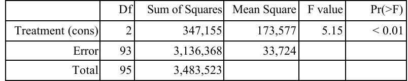
Table 4.3 Analysis of Variance table for reaction times in Pitt_Shoaf1.txt.
95 3,483,523 Total
33,724 3,136,368
93 Error
< 0.01 5.15
173,577 347,155
2 Treatment (cons)
Pr(>F) F value
Mean Square Sum of Squares
Df
Table 4.3 shows the analysis of variance table for the Pitt & Shoaf reaction time data (one
observation per listener). The F value is the ratio between variance calculated from the treatment effects (MStreatment) and the pooled variance of the observations within each treatment
(MSerror). This value should be equal to 1 (MSt = MSe) if there are no treatment effects in the data. The observed F value for this data set is so large that it is unlikely that these data could have been generated by a “no treatments” model - the differences between the treatments are too large to be the result of random differences.
assumes that the error values εij are normally distributed and independent from each other. In practice, these assumptions are approximately correct psycholinguistic data, and when the assumptions aren’t exactly met by psycholinguistic data, the mismatch between model assumptions and data isn’t enough to cause concern (ANOVA is actually pretty robust in the face of assumption violations, except that the independence assumption turns out to be very important. We’ll discuss this further in a later section).
---R note. The data for this first illustration are in the file “Pitt_Shoaf1.txt”. The reaction time measurements are in the column “rt”, and the list position is indicated in column “position”.
> ps1 <- read.delim(“Pitt_Shoaf1.txt”, sep=” “) > attach(ps1)
There are thirty-two (r = 32) instances of each of three (t = 3) positions. I extracted this data from Pitt & Shoaf’s larger data set by arbitrarily assigning the 96 listeners to either the early, mid, or late groups and then taking a single reaction time measurement from each listener’s data. This arbitrary selection of data defeats Pitt & Shoaf’s careful construction of test lists that put each word in each position an equal number of times. Later in the chapter we will use the full controlled data set in a repeated measures ANOVA. Although the data are more variable taking one observation from each listener, the conclusions that we draw from them are the same.
Recall that the definition of variance is:
€
var(x)= (xij−x ..)
2
∑
rt−1where r is the number of observations in each treatment and t is the number of treatments.
The reason for dealing in squared deviations rather than variance in analysis of variance is that we can linearly partition the sum of squared deviations into deviations due to differences between the treatments (table 4.2) and to deviation within treatment conditions without worrying about the divisors that are used in calculating variance. We are working here with squared deviations from the mean, and if you will recall, the variance of a data set is the average of the squared deviations from the mean - the sum of squared deviations divided by the number of observations in the dataset. Therefore, if we know the variance in a dataset we can calculate the sum of squared deviations by multiplying the variance times the degrees of freedom.
€
SS
tot=
∑
(
x
ij−
x
..)
2=
(
rt
−
1) var(
x
)
I used this association between variance and sum of squared deviations (SS = variance * df) to calculate the SSerror for this VOT dataset. It is:
> var(rt[position=="early"])*30 + var(rt[position=="mid"])*31 + var(rt[position=="late"])*32
[1] 3136368
The total sum of squared deviations (SStot) in the data set can also be calculated from the variance. There are 96 measurements in the dataset so the degrees of freedom is 95. You should notice that these two numbers are in table 4.3.
> var(rt)*95
[1] 3483523
Subtract SSerror from SStot to get SStreatment or calculate the treatment effect from table 4.2. Either way we get about the same answer (the uneven number of observations in different list positions complicates this slightly).
Naturally, you don’t have to do these calculations to do analysis of variance in R. There is a way of reporting, or summarizing a linear equation model to give the analysis of variance table. This is the same lm() that we used to perform linear regression in the last chapter. It is clearly a very versatile function.
> anova(lm(rt~position,data=ps1)) Analysis of Variance Table
Response: rt
Df Sum Sq Mean Sq F value Pr(>F) position 2 347155 173577 5.1469 0.007586 ** Residuals 93 3136368 33724
---Signif. codes: 0 ‘***’ 0.001 ‘**’ 0.01 ‘*’ 0.05 ‘.’ 0.1 ‘ ’ 1 >
Shadowing times from the middle and end of the list were not reliably different from each other [t(63)=1.3, p=0.189].
> t.test(rt[position=="early"],rt[position=="mid"],var.equal=T)
Two Sample t-test
data: rt[position == "early"] and rt[position == "mid"] t = 2.0621, df = 61, p-value = 0.04346
alternative hypothesis: true difference in means is not equal to 0 95 percent confidence interval:
2.509136 163.027154 sample estimates:
mean of x mean of y 888.5806 805.8125
> t.test(rt[position=="early"],rt[position=="late"],var.equal=T)
Two Sample t-test
data: rt[position == "early"] and rt[position == "late"] t = 3.0401, df = 62, p-value = 0.003462
alternative hypothesis: true difference in means is not equal to 0 95 percent confidence interval:
50.39623 243.91657 sample estimates: mean of x mean of y 888.5806 741.4242
---4.2. Two factors - interaction.
Now, the finding that reaction time is slower at the beginning of an experiment than at the end may simply suggest that listeners get better at the task, and thus have nothing to do with a response strategy. Pitt & Shoaf thought of this too and added a condition in which the prime and the target do not overlap at all. Contrasting this no overlap condition at the beginning, middle and end of the experiment with the 3-phone overlap condition that we examined above will give a clearer picture as to whether we are dealing with a practice effect (which should affect all responses) or a phonological priming effect (which should affect only the overlap trials).
overlap factor (zero vs three phones overlap between the prime and the target), and the list position factor (trials early, mid, and late in the experiment). Their argument was that if
[image:11.612.186.402.239.330.2]phonological overlap affects lexical processing in general then the effect of overlap should be seen throughout the experiment. Instead, Pitt & Shoaf found an interaction: that the overlap effect was only present in the first part of the trial list.
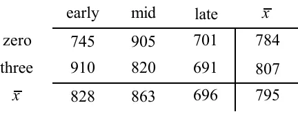
Table 4.4. Two factors in a study of phonological priming.
863 820 905 mid
795 696
828
€
x
807 691
910 three
784 701
745 zero
€
x late
early
The model tested in this two-factor analysis is:
€
x
ijk
=
µ +
α
i
+
β
j
+
α
i
β
j
+
ε
ijk
The αi and βj effects are exactly analogous with the τi (treatment) effect that we examined in the
one-factor ANOVA of section 4.1. The estimated variance (MSposition and MSoverlap in our example) is derived by comparing treatment means (the row and column means in table 4.4) with the grand mean. The sum of square total, SStot, is also caluclated exactly as in section 4.1. The interaction effect αiβj though is new. This effect depends on the interaction of the two factors α
and β.
---A note on effects. In the two factor analysis of variance, we have two main effects (a and b) and one interaction effect (ab). It is pretty easy to compute each one of the coefficients in the model directly off of the average values in table 4.4. For example, the effect for three-phone overlap is
α[3] = 807 - 796 = +11, the difference between the RT of overlap trials and the overall average
RT in the data set. The other main effect coefficients are calculated in the same way, subtracting the actual value from the predicted value. Note that the treatment effects coefficients for an effect sum to 0.
β[early] = 828 - 795 = +32.2 β[mid] = 863 - 795 = +67.1 β[late] = 696 - 795 = -99.3
The interaction effects can also be easily calculated now that we have the main effects. For instance, given our main effects for position and overlap we expect the RT for early 3-phone overlapped trials to be 839 - the overall mean (795 ms) plus the effect for overlap (+11.6 ms), plus the effect for being early in the list (+32.2 ms). The actual average RT of 3-phone
overlapped trials early in the list was 910 ms, thus the interaction term α[3]β[beg] is 910 - 839 = 71 ms.
€
RT
[ 3][beg]k=
µ
+
α
[ 3]+
β
[beg]+
α
[ 3]β
[beg]+
ε
=
795
+
12
+
32
+
71
+
ε
=
910
+
ε
It is useful to look at the size of the effects like this. The position effect is larger than the overlap effect while the interaction is the largest effect of all. You can work out the other interaction effect terms to see how symmetrical and consistently large they are.
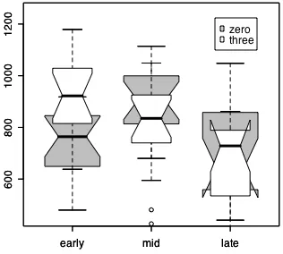
---The shadowing time data distributions are shown in figure 4.1. As we saw when we looked at the 3-phone overlap data, shadowing times seem to be longer in the 3-phone overlap trials early in the experiment but not later. Now comparing data from a control condition - trials that have no overlap between the prime and the target - we can test whether the faster shadowing times that we see in the later 3-phone overlap trials are a result of a general improvement over th course of the experiment. In the general improvement case we would expect the no-overlap data to pattern with the 3-phone overlap data. This is a test of an interaction - do the factors list position and overlap interact with each other? The “general improvement” hypothesis predicts that there will be no interaction - the overlap conditions will show the same pattern over the different list positions. The “something is going on with overlap” hypothesis predicts that the pattern over list positions will be different for the no overlap and 3-phone overlap trials. This means that the interaction terms α[3]β[beg], α[3]β[mid], α[3]β[end], etc. will be different from
Figure 4.1. Shadowing time for no overlap (gray) and 3-phone overlap (white) phonological priming, as a function of list position (a subset of data from Pitt & Shoaf, 2002, experiment 2).
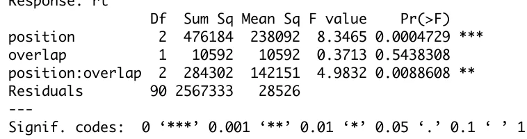
The analysis of variance (table 4.5) of this subset of the Pitt & Shoaf (2002, experiment 2) data suggests that there is a reliable interaction. We find a significant main effect of position [F(2,90) = 8.6, p < 0.01] and more importantly for the test distinguishing our two hypotheses we find a reliable interaction between position and overlap [F(2,90)=4.7, p<0.02]. This crucial interaction is shown in Figure 4.1.
Table 4.5. Two factor analysis of variance of the “Pitt_Shoaf2.txt” dataset. The R command to produce this table was: anova(lm(rt~position*overlap, data=ps2)).
Response: rt
Df Sum Sq Mean Sq F value Pr(>F) position 2 476184 238092 8.3465 0.0004729 *** overlap 1 10592 10592 0.3713 0.5438308 position:overlap 2 284302 142151 4.9832 0.0088608 ** Residuals 90 2567333 28526
---Signif. codes: 0 ‘***’ 0.001 ‘**’ 0.01 ‘*’ 0.05 ‘.’ 0.1 ‘ ’ 1
A set of planned comparisons between the no overlap “control” data and the 3-phone overlap phonological priming data indicate that the 3-phone overlap pairs were shadowed more slowly than the no overlap prime-target pairs at the beginning of the experiment [t(26.7) = -3.4, p<0.01], while the no overlap and 3-phone overlap conditions did not differ from each other in the middle of the experiment [t(29.2) = 1.4, p=0.18] and at the end of the experiment [t(30)=0.29, p=0.78].
---R note. The data for this section are in the file “Pitt_Shoaf2.txt”. As with Pitt_Shoaf1.txt, I took only a single reaction time measurement from each listener in the experiment for the dataset in Pitt_Shoaf2.txt. We have six groups (3 positions X 2 overlaps), each of which is made up of 16 listeners. The selection of which listeners would be in each group was done arbitrarily.
> detach(ps1)
> ps2 <- read.delim("Pitt_Shoaf2.txt", sep=" ") > attach(ps2)
The factor() function is used to put the levels of the “position” factor into a sensible (nonalphabetic) order so Figure 4.1 will look right.
[image:14.612.102.481.110.210.2]> ps2$position <- factor(ps2$position,levels=c("early","mid","late"))
Figure 4.1 was created using the boxplot() procedure. The first call plots the gray boxes for the subset of shadowing times where there was no phonological overlap between prime and target. The second call adds narrower white boxes plotting the distributions of times when the overlap was three phones.
> boxplot(rt~position,data=ps2,notch=T, col="gray", subset=overlap=="zero", boxwex=0.7, ylim=c(450,1250))
> boxplot(rt~position,data=ps2,notch=T, col="white", subset=overlap=="three", boxwex=0.5, add=T)
Boxplot() produces a “box and whisker” summary of the data distributions. The box has a notch at the median and covers the first and third quartiles of the distribution. This means that 50 percent of the data points lie within the box. The whiskers extend out to the largest and smallest data values unless they are beyond 1.5 times the length of the box away from the box, in which case the outlier data values are plotted with dots. So what we see in figure 4.1 is a representation of six distributions of data.
The planned comparisons that explore the position X overlap interaction are shown below. Note that I used the subset syntax to select RT measurements to include in the tests. For example, rt[position==”early” & overlap==”zero”] selects the reaction times for the 16 listeners who were selected to represent the no overlap, early condition.
> t.test(rt[position=="early" & overlap=="zero"],rt[position=="early" & overlap=="three"])
Welch Two Sample t-test
data: rt[position == "early" & overlap == "zero"] and rt[position == "early" & overlap == "three"]
t = -3.4015, df = 26.669, p-value = 0.002126
alternative hypothesis: true difference in means is not equal to 0 95 percent confidence interval:
-278.23698 -68.78802 sample estimates:
mean of x mean of y 744.6875 918.2000
---4.3 Repeated measures
As I mentioned in section 4.1, the analyses described in sections 4.1 and 4.2 assume that each observation in the data set is independent from the others, and made it this way by selecting data from Pitt & Shoaf’s raw data files following the sampling plan shown in table 4.1.
study, we collect six reaction time values from each listener. Recall that I said that the “no overlap” condition was added as a control to help guide our interpretation of the 3-phone overlap condition. In the independent observations scheme of table 4.5 listeners S1, S2, and S3 provide the control reaction times which will then be compared with the reaction times given by listeners S4, S5, and S6. Thus, any individual differences between the listeners (alertness level, motivation, etc.) contribute to random unexplained variation among the conditions. When we compare
[image:16.612.72.538.282.427.2]listener S1’s reaction times in the six conditions, though, we have a somewhat more sensitive measure of the differences among the conditions because presumably his/her alertness and motivation is relatively constant in the test session.
Table 4.6. Data sampling plan using repeated measures - six observations per listener.
x12 x11 x10 x9 x8 x7
and so on...
x6 x5 x4 x3 x2 3-phone overlap S6 S5 S4 S3 x1 S2 S1 late mid early late mid early no overlap
The statistical complication of the repeated measures sampling scheme is that now the individual observations are not independent of each other (e.g. x1-6 were all contributed by S1) so the standard analysis of variance cannot be used.
We saw in chapter 3 that if you have two measurements from each person you can use a paired t test instead of an independent samples t test and the test is much more powerful because each person serves as his/her own control. Recall, in the paired t test the overall level for a person may be relatively high or low but if people with slow reaction times show a difference between conditions and people with fast reaction times also show a difference, then the overall difference between people doesn’t matter so much - the paired comparison tests the difference between conditions while ignoring overall differences between people.
In a dataset with more than one observation per person, the observations all from one person (within subject) are often more highly correlated with each other than they are with
observations of other people. For example, in reaction time experiments subjects typically differ from each other in their average reaction time. One person may be a bit faster while another is a bit slower. It may be that despite this overall difference in reaction time an experimental
manipulation does impact behavior in a consistent way for the two subjects.
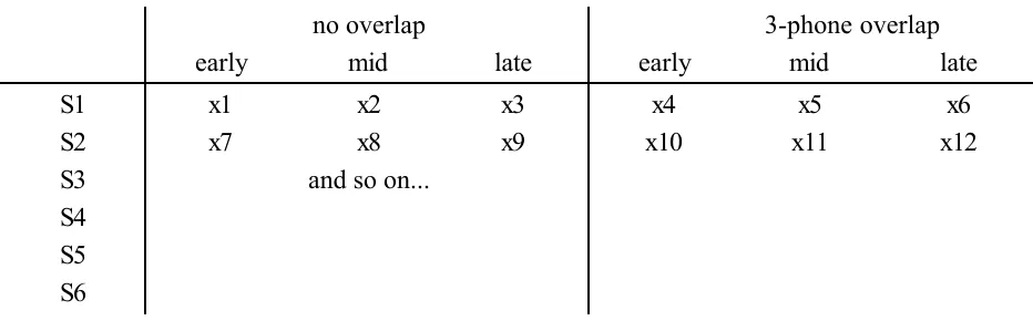
Here’s an illustration using hypothetical data to show how repeated measures analysis of
variance works. If we want to know if an effect is consistently present among the participants of a study we need to look at the subjects individually to see if they all show the same pattern. This is shown in the comparison of two hypothetical experiments in Figures 4.2 and 4.3. In these hypothetical data we have two experiments that resulted in the same overall mean
difference between condition A and condition B. In condition A the average response was 10 and in condition B the average response was 20. However, as the figures make clear, in experiment 1 the subjects all had a higher response for condition B than condition A, while in experiment 2 some subjects showed this effect and some didn’t.
5 10 15 20 25
A
B
Experiment 1
Response
[image:17.612.132.480.374.675.2]condition
in condition B was 20. In this hypothetical experiment the subjects (each of which is plotted individually) showed the same basic tendency to have a higher response in condition B. Thus the condition by subjects interaction is relatively small.
0 5 10 15 20 25 30
A
B
Experiment 2
Response
[image:18.612.128.485.259.572.2]Condition
Figure 4.3. In this experiment the average response in condition A was again 10 and the average response in condition B was 20, but this time there was a subset of subjects (marked with filled symbols) who showed the opposite trend from that shown by the majority of the subjects.
independent observations ANOVA was F(1,30) = 212, p < 0.01, and for experiment 2 it was F(1,30)=13.2, p < 0.01. However, when we conduct the ANOVA with repeated measures we find that the difference between conditions A and B was significantly greater than chance in experiment 1 [F(1,15) = 168, p < 0.01] while this distinction was less reliable in experiment 2 [F(1,15)=7, p = 0.018]. The inconsistency among subjects in realizing the AB contrast results in a lower likelihood that we should conclude that there is a real difference between A and B in this population even though the average difference is the same.
---R note. The comparison of the hypothetical experiments 1 and 2 (figures 4.2 and 4.3) was done with the following R commands.
e12 <- read.delim("exp1versusexp2.txt") # read the data
e12$subj <- factor(e12$subj) # treat subject as a nominal variable e1 <- subset(e12,experiment=="exp1") # get the exp1 data
e2 <- subset(e12,experiment=="exp2") # get the exp2 data
# an incorrect analysis of variance - yes R lets you make mistakes anova(lm(response~condition,data=e1)) # incorrect!!!!
To see what is happening in the repeated measures analysis - the correct analysis with (subj) as the error term in the test of the condition main effect, look at these three ANOVA tables. First, we have a test of lm(response~condition, data=e2).
Df Sum Sq Mean Sq F value Pr(>F) condition 1 736.80 736.80 13.261 0.001012 ** Residuals 30 1666.85 55.56
The F value here is 736.8 divided by 55.6. The error term, 55.6, is the variance of the data values around the means of conditions A and B, incorrectly treating each observation as if it is independent of all the others. We saw in Figure 4.4 that the subjects were not consistent in their responses to the A/B contrast, so we might expect the interaction between condition and subject to be large in this data set. The table produced by lm(response~condition*subj) shows a pretty large MS value (variance) attributable to the condition:subj interaction, as we would expect because the subjects showed different patterns from each other.
To test whether the condition main effect was consistent across subjects we use the MS for the
condition:subj interaction as the denominator (error term) in the F ratio. In this case that means that we would take F(1,15) = 736.8/105.16 = 7. Note that the variance due to condition is the same in both the repeated measures analysis (with condition:subj as the error term) as it is in the non-repeated measures analysis (with the residual mean square as the error term). The only change is in the selection of the error term. The correct error term is selected automatically in R using aov() with subject specified as the error variable, and that we have repeated measures over the factor condition.
> summary(aov(response~condition+Error(subj/condition),data=e2))
Error: subj
Df Sum Sq Mean Sq F value Pr(>F) Residuals 15 89.382 5.959
Error: Within
Df Sum Sq Mean Sq F value Pr(>F) condition 1 736.80 736.80 7.0062 0.01830 * Residuals 15 1577.47 105.16
This analysis uses the MS for the condition:subj interaction as the error term (denominator) in the F ratio testing whether there was a reliable or consistent effect of condition. And in general the key method in repeated measures analysis of variance, then, is to test the significance of an effect with the effect:subjects interaction as the error term in the F ratio. The aov() function with its option to specify the Error term simplifies the analysis of complicated designs in which we have several within-subjects factors (for which we have repeated measures over each participant) and between-subjects factors (for which there were different groups of people).
---4.3.1 An example of repeated measures ANOVA
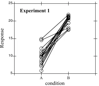
Now, at long last, we can analyze Pitt & Shoaf’s (2002) data. Figure 4.4 shows the shadowing time distributions for all of the critical trials at the beginning, middle, and end of the experimental session, for no overlap prime/target pairs and for 3-phone overlap pairs. The pattern that we saw in sections 4.1 and 4.2 is now quite clear. Responses in the early 3-phone overlap trials are longer than any of the other responses which are centered around 800 ms. We found with a subset of these data that there was an interaction between position and overlap and it looks like that will be the case again, but how to test for it?
Notice from the analysis of variance table produced with this model (rt ~ position*overlap*subj) that there are no F values. This is because all of the variance in the data set is covered by the variables - by the time we get to the early, no overlap reaction time produced by subject S1 there is only one value in the cell - and thus no residual variance between the model predictions and the actual data values.
Figure 4.4. Phonological priming effect contrasting trials with 3-phones
This is just as well, because the analysis of variance table in table 4.7 is incorrectly based on the assumption that the observations in the dataset are independent of each other. We need to perform a repeated measures analysis. At this point we can either use the values in table 4.7 to compute the repeated measures statistics by hand, or use a different R call to compute the repeated measures statistics for us. It isn’t hard to compute the F values that we are interested in. The position main effect is MSp/MSp:s = 55829/25967 = 2.15. The overlap main effect is
[image:22.612.71.507.296.467.2]MSo/MSo:s = 19758/15566 = 1.27. And the position by overlap interaction is MSp:o/MSp:o:s = 142212/14051 = 10.12.
Table 4.7. Analysis of variance table for the repeated measures analysis of Pitt & Shoaf (2002, experiment 2). The R call to produce this table was:
anova(lm(rt~position*overlap*subj,data=ps3)) 0 0 Residuals 14051 2697804 192 position:overlap:subj 15566 1494378 96 overlap:subj 25967 4985721 192 position:subj 142212 284424 2 position:overlap 106118 10187344 96 subj 19758 19758 1 overlap 55829 111658 2 position Pr(>F) F value Mean Sq Sum Sq Df
A call to summary(aov()) with these data, and the error term Error(subj/(position*overlap)) indicating that position and overlap are within-subject factors, produces the same F values that I calculated above, but also gives their probabilities.
Table 4.8. Repeated measures ANOVA table for Pitt & Shoaf (2002) experiment 2. The R call to produce this table was:
14051 2697804 192 position:overlap:subj <0.01 10.12 142212 284424 2 position:overlap 15566 1494378 96 overlap:subj 0.26 1.27 19758 19758 1 overlap 25967 4985721 192 position:subj 0.12 2.15 55829 111658 2 position Pr(>F) F value Mean Sq Sum Sq Df
In the earlier analysis we had a significant main effect for position as well as the significant interaction between position and overlap. With the larger set of data it becomes apparent that the interaction is the more robust of these two earlier findings.
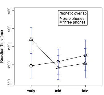
Naturally, we want to explore these findings further in a planned comparison or post-hoc test. However the t-tests that we used earlier assume the independence of the observations, and since we have repeated measures we can’t use t-test to explore the factors in more detail. The usual strategy at this point in psycholinguists is to perform another repeated measures ANOVA on a subset of the data. For example, I looked at the effect of overlap for the early, mid, and late trials in three separate repeated measures ANOVAs and found a significant difference between no overlap and 3-phone overlap conditions in the early list position [F(1,96)=21, p<0.01], but no significant phonological priming effects at the middle [F(1,96)=1.3, p=0.25] or end
[F(1,96)=1.16, p=0.28] of the experiment. These analyses suggest that the first few trials involving a substantial amount of phonetic overlap between prime and target are in some sense surprizing to the listener resulting in a delayed shadowing response.
Figure 4.5. Response to phonological overlap between prime and target in Pitt & Shoaf (2002) experiment 2, as the experiment progressed from the first bin of 7 trials to the end.
---
---R-note. Specifiying the Error term in the aov() command is a little tricky. For example, the specification Error(subj/position*overlap) is interpreted to mean that we want to test for a set of error terms - subj:position, overlap, and subj:position:overlap. This is not quite right. We want subj:position, sub:overlap, and subj:position:overlap and to get this set of error terms we need to specify the error term as Error(subj/(position*overlap)) - that position and overlap are both within-subject factors.
When the number of observations in each cell of the model is not equal, the printout from aov() includes a number of additional tests. The wanted F values ARE printed and can be checked against the simple anova(lm()) printout, so I just ignore the extraneous tests given by aov().
Error: subj
Df Sum Sq Mean Sq F value Pr(>F) Residuals 96 10187344 106118
Error: subj:position
Df Sum Sq Mean Sq F value Pr(>F) position 2 111658 55829 2.15 0.1193 Residuals 192 4985721 25967
Error: subj:overlap
Df Sum Sq Mean Sq F value Pr(>F) overlap 1 19758 19758 1.2692 0.2627 Residuals 96 1494378 15566
Error: subj:position:overlap
Df Sum Sq Mean Sq F value Pr(>F) position:overlap 2 284424 142212 10.121 6.623e-05 *** Residuals 192 2697804 14051
---Signif. codes: 0 ‘***’ 0.001 ‘**’ 0.01 ‘*’ 0.05 ‘.’ 0.1 ‘ ’ 1
The planned comparisons that I performed with this repeated measures ANOVA was done by taking a subset of data, and then performing a one-way ANOVA on the subset, still using the subject:overlap mean square as the error term since we have repeated measures on the items being compared.
> subset(ps3,c(position=="early")) -> ps3.early
> summary(aov(rt~overlap+Error(subj/overlap),data=ps3.early))
Error: subj
Df Sum Sq Mean Sq F value Pr(>F) Residuals 96 4133049 43053
Error: subj:overlap
Df Sum Sq Mean Sq F value Pr(>F) overlap 1 266252 266252 21.55 1.093e-05 *** Residuals 96 1186098 12355
[image:25.612.75.462.99.384.2]---Signif. codes: 0 `***' 0.001 `**' 0.01 `*' 0.05 `.' 0.1 ` ' 1
from CRAN using the “package installer”. Once it is downloaded you use the library() function to make the functions in the package available in your R session. Here are the commands that I used for Figure 4.4.
> plotmeans(rt~position,data=ps3, subset=(overlap=="zero"), n.label=F, ylim=c(750,950), ylab="Reaction Time (ms)", xlab="", cex=2)
> plotmeans(rt~position,data=ps3, subset=(overlap=="three"), n.label=F, cex=2, pch=2, add=T)
> legend(2,950,title="Phonetic overlap",legend=c("zero phones","three phones"),pch=c(1,2))
---4.3.2 Repeated Measures ANOVA with a between-subjects factor.
Here’s another quick example of repeated measures ANOVA, this time with a between-subjects grouping variable. We’re using a data set of reaction times in an AX phonetic discrimination task. Listeners hear two sounds and press either the “same” button if the two are identical or the
“different” button if the two sounds are different in any way.
The raw data (correct responses only) were processed to give the median reaction time
measurement for each listener for each pair of sounds presented. These are our estimates of how long it took each person to decide if the pair is the same or different, and we think that this is a good measure of how different the two sounds are. So each listener is measured on each of the pairs of sounds. This is our “within-subjects” repeated measurements variable because we have repeatedly measured reaction time for the same person, and we have an estimate of reaction time for each listener on each of three different pairs of sounds.
We also have one “between-subjects” variable because we have four groups of listeners - American English native speakers who never studied Spanish, have a beginner’s knowledge of Spanish, or have an “intermediate” knowledge of Spanish, and then a group of Latin American Spanish native speakers.
When I analyzed this data in SPSS I set the data up so that there was one line for each listener. So subject 229, who is in the “beginning Spanish” group of listeners had a median RT for the same pair /d/-/d/ of 645 milliseconds, for the different pair /d/-/D/ of 639, and so on.
begin 234 746.0 781.5 719.5 704.0 768.0 715.0 begin 235 800.5 708.5 668.0 708.0 663.0 719.5 begin 236 582.0 849.5 596.0 557.5 629.5 585.0
The SPSS “repeated measures” analysis produced using this data organization is very complete. Here’s what I did to produce a similar analysis in R.
Note, this analysis style has the advantage that if you test several within subjects factors the data file is easier to produce and manage.
1) Organize the data with a single column for the dependent measure - MedianRT, and a column also for each independent measure. I used the E-Prime utility program “Data Aid” to produce this data file. You can also use a spreadsheet program, just remember that R wants to read files in raw .txt format. Here are the first few lines of the data file.
group pair listener MedianRT begin d_d 229 645.0 begin d_d 230 631.0 begin d_d 234 746.0 begin d_d 235 800.5 begin d_d 236 582.0 begin d_d 247 646.0 begin d_d 250 954.0 begin d_d 252 692.5 begin d_d 253 1080.0
2) Read the data into R.
> spaneng <- read.delim("spanengRT.txt") > spaneng$listener <- factor(spaneng$listener)
3) Take a subset of the data - just the “different” pairs. I could have done this in step 1) above, but it isn’t too hard to do it in R either.
> speng.subset <- subset(spaneng, pair == "d_r" | pair == "d_th" | pair == "r_th", select=c(group,pair,listener,MedianRT))
making this a repeated measures analysis.
> summary(aov(MedianRT~pair*group+Error(listener/pair),data=speng.subset))
Error: listener
Df Sum Sq Mean Sq F value Pr(>F) group 3 461500 153833 3.3228 0.02623 * Residuals 55 2546290 46296 ---
Signif. codes: 0 `***' 0.001 `**' 0.01 `*' 0.05 `.' 0.1 ` ' 1
Error: listener:pair
Df Sum Sq Mean Sq F value Pr(>F) pair 2 121582 60791 47.9356 1.069e-15 *** pair:group 6 38001 6334 4.9942 0.0001467 *** Residuals 110 139500 1268 ---
Signif. codes: 0 `***' 0.001 `**' 0.01 `*' 0.05 `.' 0.1 ` ' 1
I’ll leave as an exercise for the reader to explore the “pair by group” interaction further with planned comparisons and graphs. Here’s one way to graph the results of this experiment.
> plotmeans(MedianRT~pair,data=speng.subset,subset=group=="nospan", n.label=F, ylim=c(600,950), ylab="Reaction Time (ms)",cex=2)
> plotmeans(MedianRT~pair,data=speng.subset, subset=group=="spannat", n.label=F, cex=2,add=T,pch=2,)
---4.4 The “language as fixed effect” fallacy.
words or sentences1 .
I will use an interesting data set donated by Barbara Luka (Psychology, Bard College) to illustrate the use of two F values to test every effect - the subjects analysis and the items analysis. Following Clark ‘s (1973) suggestion we will combine F values found in the subjects analysis and F values from the items analysis to calculate the minF’ - our best estimate of the reliability of effects over people and sentences. Luka and Barsalou (2005) tested whether subjects’ judgement of the grammaticality of a sentence would be influenced by mere exposure to the sentence, or even by mere exposure to a sentence that has a similar grammatical structure to the one they are judging. In their experiment 4, Luka and Barsalou asked participants to read a set of sentences outloud for a tape recording. Then after a short distractor task (math problems) they were asked to rate the grammaticality of a set of sentences on a scale from 1 “very ungrammatical” to 7 “perfectly grammatical”. One half of the 48 sentences in the grammaticality set were related in some way to the sentences in the recording session - 12 were exactly the same, and 12 were structurally similar but with different words. Half of the test sentences were judged in a pretest to be highly grammatical and half were judged to be moderately grammatical.
(1) highly grammatical
reading task It was simple for the surgeon to hide the evidence. identical It was simple for the surgeon to hide the evidence. structural It is difficult for Kate to decipher your handwriting.
(2) moderately grammatical
reading task There dawned an unlucky day. identical There dawned an unlucky day. structural There erupted a horrible plague.
After the experiment was over Luka and Barsalou asked the participants whether they noticed the identical and structural repetition. 22 of 24 said they noticed the identical repetitions and 18 of 24 said that they noticed the structural repetitions - saying things like “grammatical errors were alike in both sections” or “wording of the sentences was in the same pattern”, but also “same type of words”. So, just as with the Pitt & Shoaf (2002) phonological priming study, the participant’s awareness of repetition and perhaps strategic response to the repetition may be a factor in this experiment.
In a nutshell (see figure 4.6), what Luka and Barsalou found is that repetition, either identical or structural, results in higher grammaticality judgements. This finding is rather interesting for a
1 Raaijmakers et al. (1999) emphasize that it is important to report the minF’, which will be discussed later in this
couple of different reasons, but before we get to that let’s talk about how to test the result. The first step is that we conduct a repeated measures analysis of variance with repetitions over subjects. Luka & Barsalou did this by taking the average rating for each person in the experiment, for each combination of factors - familiarity, grammaticality, and type of repetition. This results in eight average rating values for each subject, corresponding to the eight boxes in figure 4.6. Keep in mind here that we are averaging over different sentences, and acting as if the differences between the sentences don’t matter. This is OK because later we will pay attention to the differences between the sentences.
The “subjects” analysis then is a repeated measures analysis of variance exactly as we have done in each of the examples in section 4.3. Using the raw rating data we get exactly the same F values reported by Luka & Barsalou (2005). I decided to use the arcsine transform with these data because the rating scale has a hard upper limit and ratings for the “highly grammatical” sentences were smooshed up against that limit, making it difficult to measure differences between
sentences. In this analyis, as in Luka & Barsalou’s analysis, we have main effects for
grammaticality [F1(1,25)=221, p<0.01] and familiarity [F1(1,25)=10.5, p<0.01]. Two effects
came close to significant (this analysis is using α=0.01 as the critical value): repetition type
[F1(1,25)=5.6, p<0.05], and the three-way interaction between grammaticality, familiarity, and
repetition type [F1(1,25)=3.7,p=0.06]. Notice that in this report I am using the symbol F1 in place of plain F. Following Clark (1973), this is the usual way that psycholinguists refer to the F values obtained in a subjects analysis. The items analysis F values are written with F2 and in general we expect that if we are going to claim that we have found an effect in the experiment it must be significant in both the subject analysis and in the item analysis and the minF’
Figure 4.6. Results of Luka & Barsalou (2005) experiment 4. The two boxes on the left show results for the highly grammatical sentences, while the two boxes on the right are for the moderately grammatical sentences. Within these groupings the identical repetitions are on the left and the structural repetitions are on the right. Gray boxes plot the grammaticality rating when then sentence was repeated (identically or structurally) and white boxes plot the ratings when the same
sentence was not primed during the reading portion of the experiment.
The items analysis of these grammaticality rating data has repeated measures over just one factor. Sentences were reused in different lists of the materials so that each sentence was presented half the time as a novel sentence and half the time as a repeated sentence (either structural repetitition or identical repetition). Obviously Luka & Barsalou couldn’t have used the same sentence in both the highly grammatical condition and in the moderately grammatical condition, so
This analysis, again using the arcsine transform to make the data distributions more normal, found the same two significant effects that we found in the subjects analysis. Highly grammatical sentences were judged to be more grammatical than the moderately grammatical sentences
[F2(1,43)=77, p<0.01]. This indicates that the participants in the experiment agreed with the
participants in the pretest (whose judgements were used to determine the grammaticality category of each sentence). There was also a significant effect of familiarity [F2(1,43)=9.4, p<0.01]. New items had an average familiarity rating of 5.6 while repeated items (averaging over identical repetition and structural repetition) had a higher average rating of 5.8. This increased “grammaticality” for repeated sentences and sentence structures was found to be significant in both the subjects analysis and in the items analysis.
Now we combine the information from the subjects analysis and the items analysis to calculate the minF’ - the ultimate measure of whether the experimental variable had a reliable effect on responses, generalizing over both subjects and items. MinF’ is an estimate of the lower limit of the statistic F’ (F-prime) which cannot usually be directly calculated from psycholinguistic data. This statistic evaluates whether the experimental manipulations were reliable over subjects and items simulataneously. I would say at this point that the minF’ statistic is a high bar to pass. Because minF’ is a lower-limit estimate, telling us the lowest value F’ could have given the
separate subjects and items estimates, it is a conservative statistic which requires strong effects in both subject and items analyses (which means lots of items). In experiments where the items are matched across conditions or counter-balanced across subjects, it may not necessary to use items analysis and the minF’ statistic. See Raaijmakers et al. (1999) for guidance.
To calculate minF’ divide the product of F1 and F2 by their sum:
€
minF'
=
F
1
*
F
2
F
1
+
F
2
The degrees of freedom for the minF’ is also a function of the subjects and items analyses:
€
df
=
(
F
1
+
F
2
)
2
F
1
2
*
n
2
+
F
2
2
*
n
1
In this formula, n1 is the degrees of freedom of the error term for F1 and n2 is the degrees of freedom of the error term for F2.
Table 4.9 shows the results of the minF’ analysis of Luka and Barsalou’s data. Both the
[image:33.612.189.426.284.407.2]grammaticality and familiarity main effects are significant in the minF’ analysis, just as they were in the separate subjects and items analyses, but the minF’ values make clear that the repetition type effect which was significan by subjects and somewhat marginally significant in the items analysis (p=0.195) is not even being close to significant.
Table 4.9. MinF’ values (and the error degrees of freedom) in the analysis of Luka and Barsalou’s data. The F values found in the subjects analysis are shown in the first column. The second column shows the F values from the items analysis. F values that are significant at p< 0.05 are underlined.
65 0.95 1.3 3.7 gram*fam*rep 45 1.00 3.5 1.4 fam*rep 63 1.32 1.7 5.6 repetition type
65 4.96 9.4 10.5 familiarity 65 57.10 77.0 221.0 grammaticality df minF’ F2 F1
Before wrapping up this chapter I would like to say that I think that Luka and Barsalou’s (2005) finding is very interesting for linguistics because it suggests that grammaticality is malleable -that “mere exposure” tends to increase the acceptability of a sentence structure. Additionally, it is interesting to me that it is structure that seems to be exposed in these sentences because there were no reliable differences between the identical repetitions and the structural repetitions and because the identical repetitions are also structural repetitions. The implication is that sharing the words in the repetition added nothing to the strength of the repetition effect. The picture of syntactic knowledge that seems to emerge from this experiment (and others like it in the literature) is that syntactic knowledge is about structures rather than exemplars, and yet that it emerges gradiently from exposure to exemplars.
> LB1 <- read.delim("LukaBars05Exp4_subj.txt") > LB1$SUBJ <- factor(LB1$SUBJ)
> summary(aov(2/pi*asin(sqrt((RATING/7)))~GRAMMATICALITY*FAMILIARITY*
TYPE.TOKEN+Error(SUBJ/(GRAMMATICALITY*FAMILIARITY*TYPE.TOKEN)),data=LB1))
Note that I’m using the arcsine transform for this analysis. I felt that this was appropriate because the rating scale has a strict maximum value and there was a good deal of compression at the top of the range for the highly grammatical sentences. The arcsine transform expands the scale at the top so that rating differences near 7 will come out.
The items analysis uses a different data file which has the average rating value (averaged over subjects) for each test sentence. Different test sentences were used for the grammaticality and type.token experimental factors, so the only repeated factor was familiarity. That is the same sentence was used (with different participants) as a novel or repeated sentence.
> LB2 <- read.delim("LukaBars05Exp4_items.txt") > LB2$Item <- factor(LB2$Item)
> LB2 <- na.omit(LB2) # one sentence had to be omitted
> summary(aov(2/pi*asin(sqrt(RATING/7)) ~ GRAMMATICALITY * FAMILIARITY * REPETITION + Error(Item/FAMILIARITY),data=LB2))
Finally, for your appreciation and admiration, and so I’ll have something to refer back to in similar cases, the lines below were used to create figure 4.6. To keep the “boxplot” statements relatively clean I used subset to select data for the plot statements.
> subset(LB1,FAMILIARITY=="New")->LB.New > attach(LB.New)
> boxplot(2/pi*asin(sqrt(RATING/7))~ TYPE.TOKEN + GRAMMATICALITY, notch=T, ylab="Arcsin(rating)", boxwex=0.7)
> subset(LB1,FAMILIARITY=="Old")->LB.Old > attach(LB.Old)
> boxplot(2/pi*asin(sqrt(RATING/7)) ~ TYPE.TOKEN + GRAMMATICALITY, notch=T, boxwex=0.5, col="lightgray",add=T)
> legend(2.7,0.99,legend=c("Repeated","Novel"),fill=c("gray","white"), title="Familiarity")
---Exercises.
estimates? i.e. what is the numerator in the F statistic, and what is the denominator, and why is a ratio a meaningful way to present and test the strength of a hypothesized effect?
2. In Luka and Barsalou’s (2005) experiment 4, the three way interaction grammaticality by repetition type by familiarity was almost significant in the subjects analysis. The likely cause of the three way interaction is visible in the data in figure 4.6. What aspect of the results shown in figure 4.7 would lead you to suspect that a three way interaction might be present?
3. Suppose that you analyze the results of an experiment using both subjects analysis and items analysis and find that F1 is significant F2 is not. What is going on?
4. The data file VCVdiscrim.txt is available on the book website. This “question” takes you step-by-step through a repeated measures ANOVA of this data. The interesting thing about this dataset is that it has two within subjects factors.
4.1. Use these commands to read this data into R and verify that it was read successfully.
vcv <- read.delim("VCVdiscrim.txt") vcv$Subject <- factor(vcv$Subject) summary(vcv)
4.2. vowel and pair2 are within-subjects factors. How many different listeners participated in this experiment, and how many repeated measures were taken of each listener? The table()
command may help you answer these questions.
table(vcv$Subject)
table(vcv$vowel,vcv$pair2)
4.3. Now, do a univariate non-repeated measures analysis of variance. Be very patient, it is calculating a very large covariance matrix and a regression formula with several hundred
coefficients. It didn’t die it is just working. With a long calculation like this it is helpful to save the result - I put it in a linear model object that I namedmylm.
mylm <- lm(medianRT~L.lang*pair2*vowel*Subject,data=vcv)
To see the coefficients you can type: summary(mylm)
But we are really most interested in the anova table: anova(mylm)
vowel and pair2 are within-subjects effects.
What are the error terms for the following tests, and what is the F ratio assuming those error terms?
L.lang:pair2 pair2:vowel
L.lang:pair2:vowel L.lang:vowel vowel pair2 L.lang
F MS error
MS treatment name of error term
4.4. You can find the correct answers for this table by using the aov() command with the error term: Subject/(pair2*vowel)
This calculates separate anova tables for the following error terms Subject, pair2:Subject,
vowel:Subject, and pair2:vowel:Subject. Then aov() matches these to the correct effects, just like you did in the table :)
summary(aov(medianRT~L.lang*pair2*vowel+Error(Subject/(pair2*vowel)), data=vcv))
4.5. One of the effects found in this analysis is the vowel main effect. It was also found that this effect was present for both groups of listeners (the vowel:L.lang interaction was not significant).
Look at the table of reaction times, and the (hacky) graph produced by the following commands. What would it look like for there to be an interaction in these data? (hint: you can make up data and plot it using c() the way I made up the x axis for the plot).
myv <- aggregate(vcv$medianRT,list(v=vcv$vowel,lang=L.lang),mean)
myv
plot(c(1,2,3),x[lang=="AE"],type="b",ylim=c(600,750),xlim=c(0.5,3.5))
lines(c(1,2,3),x[lang=="D"],type="b")
5. Try a repeated measures analysis of a different dataset.
This example shows the analysis of an experiment with one within-subjects varianble and one between-subjects variable. We want to know whether these two factors interact with each other. Amanda Boomershine asked Spanish speakers to judge the dialect of other Spanish speakers. The question was: “does this person speak local Spanish, or is he/she from another country?” The talkers and listeners were from Mexico and Puerto Rico. The data are in “dialectID.txt”. The dataset has four columns T.lang is the dialect of the talker (Puerto Rican or Mexican), L.lang is the dialect of the listener (PR or M), Listener is the ID number of the listener, and pcorrect is the proportion of correct responses. We have two groups of listeners so the Listener variable is “nested” within the L.lang variable (subject #1 for example only appears in listener group M).
Boomershine took repeated measures of the talker dialect variable. That is, each listener provided judgements about both Puerto Rican and Mexican talkers. So T.Lang is a “within-subjects” variable because we have data from each listener for both levels. The L.lang variable is a
“between-subjects” variable because for any one person we only have one level on that variable - each listener is either from Puerto Rico or Mexico. You should also apply the arcsine transform to the probability correct data.
2/pi*asin(sqrt(pcorrect)) # arcsine transform
dlect <- read.delim("dialectID.txt") # read the data