Stochastic control methods to individualise drug therapy by incorporating pharmacokinetic, pharmacodynamic and adverse event data

STOCHASTIC CONTROL METHODS TO

INDIVIDUALISE DRUG THERAPY BY

INCORPORATING PHARMACOKINETIC,

PHARMACODYNAMIC AND ADVERSE EVENT

DATA.

Thesis submitted in accordance with the requirements

of the University of Liverpool for the degree of Doctor

in Philosophy

by

Ben Robert Francis

There are a number of methods available to clinicians for determining an individualised

dosage regimen for a patient. However, often these methods are non-adaptive to the

patient’s requirements and do not allow for changing clinical targets throughout the course

of therapy. The drug dose algorithm constructed in this thesis, using stochastic control

methods, harnesses information on the variability of the patient’s response to the drug

thus ensuring the algorithm is adapting to the needs of the patient.

Novel research is undertaken to include process noise in the

Pharmacokinetic/Pharmacodynamic (PK/PD) response prediction to better simulate the

patient response to the dose by allowing values sampled from the individual PK/PD

parameter distributions to vary over time. The Kalman filter is then adapted to use these

predictions alongside measurements, feeding information back into the algorithm in order

to better ascertain the current PK/PD response of the patient. From this a dosage regimen

is estimated to induce desired future PK/PD response via an appropriately formulated cost

function. Further novel work explores different formulations of this cost function by

considering probabilities from a Markov model.

In applied examples, previous methodology is adapted to allow control of patients that

have missing covariate information to be appropriately dosed in warfarin therapy. Then

using the introduced methodology in the thesis, the drug dose algorithm is shown to be

adaptive to patient needs for imatinib and simvastatin therapy. The differences, between

standard dosing and estimated dosage regimens using the methodologies developed, are

wide ranging as some patients require no dose alterations whereas other required a

substantial change in dosing to meet the PK/PD targets.

The outdated paradigm of ‘one size fits all’ dosing is subject to debate and the research in

this thesis adds to the evidence and also provides an algorithm for a better approach to the

challenge of individualising drug therapy to treat the patient more effectively. The drug

dose algorithm developed is applicable to many different drug therapy scenarios due to the

enhancements made to the formulation of the cost functions. With this in mind,

application of the drug dose algorithm in a wide range of clinical dosing decisions is

possible.

Preface ____________________________________________________________ 7 Declaration _________________________________________________________ 8 1 Introduction _____________________________________________________ 9 1.1 Introduction to Individualised Drug Therapy ____________________________ 9 1.2 The Variability of Drug Response in the Population _____________________ 10 1.3 The Stages Involved in Individualising Drug Therapy ____________________ 12 1.4 The Types of Individualised Drug Therapy _____________________________ 15 1.5 The Reception of New Research into the Individualisation of Drug Therapy __ 17 2 Pharmacokinetics and Pharmacodynamics ___________________________ 20 2.1 Background Science and Basis of Translational Objective _________________ 20 2.1.1 What is Pharmacokinetics? _______________________________________________ 20 2.1.2 What is Pharmacodynamics? ______________________________________________ 21 2.1.3 The Use of Mathematical Models in Pharmacokinetics and Pharmacodynamics _____ 22 2.1.4 Data in Pharmacokinetics ________________________________________________ 23

2.2 Formulating the Pharmacometric Model ______________________________ 24 2.2.1 Modelling Methodologies ________________________________________________ 24 2.2.2 Compartmental Modelling _______________________________________________ 25 2.2.3 Commonly-used PK Parameters ___________________________________________ 27 2.2.4 Commonly-used Compartmental Models ____________________________________ 29 2.2.5 Pharmacodynamic Modelling _____________________________________________ 35

2.3 Software Packages for Pharmacometric Analysis _______________________ 38 2.3.1 Parametric Approach Software ____________________________________________ 38 2.3.2 Non-Parametric Approach Software ________________________________________ 39

3 Assessment of a Drug Dose Algorithm Not Informed by a Pharmacometric Model ____________________________________________________________ 43

3.1 A Review of A Priori Regression Models for Warfarin Maintenance Dose

Prediction ____________________________________________________________ 44 3.1.1 Introduction ___________________________________________________________ 44

3.1.2 Methods ______________________________________________________________ 48 3.1.3 Results _______________________________________________________________ 52 3.1.4 Discussion _____________________________________________________________ 57

4 Stochastic Control Methodology ___________________________________ 63 4.1 What is Stochastic Control? ________________________________________ 64 4.2 A Brief History of Control Methodologies in Drug Therapy ________________ 65 4.3 A New Approach in the Application of Stochastic Control Theory in PK/PD __ 69 4.4 Considerations for Application to Pharmacokinetics_____________________ 71 4.4.1 Preliminaries for Stochastic Control Application ______________________________ 71 4.4.2 The Mechanism of Stochastic Control in Pharmacokinetics______________________ 72

4.5 Derivation of the Cost Function Distribution ___________________________ 76 4.5.1 Prior Distributions ______________________________________________________ 76 4.5.2 The Distribution of Predicted Plasma Concentration ___________________________ 78 4.5.3 Using the Cost Function to Determine the Optimal Dosage Regimen ______________ 84

4.6 Enabling Feedback to the System ____________________________________ 86 4.6.1 Open-Loop and Closed-Loop Control _______________________________________ 86 4.6.2 Example of a System that Updates with Measurements ________________________ 88 4.6.3 Application of the Kalman filter for the dosing of lopinavir ______________________ 96

4.7 Discussion _____________________________________________________ 103 5 Stochastic Control with Pharmacokinetic Targets _____________________ 107 5.1 Example of Obtaining an Optimal IV Infusion Regimen without Feedback __ 107 5.1.1 Introduction __________________________________________________________ 107 5.1.2 Method ______________________________________________________________ 108 5.1.3 Results ______________________________________________________________ 111 5.1.4 Conclusion ___________________________________________________________ 115

5.2 Example of Obtaining an Optimal Oral Dosage Regimen with Noise Introduced and an Altered Multiple Model Approach __________________________________ 118

5.3 Example of Obtaining an Optimal Oral Regimen with Parameter Noise

Introduced and Measurements Used to Update the System ___________________ 129 5.3.1 Introduction __________________________________________________________ 129 5.3.2 Method ______________________________________________________________ 130 5.3.3 Results ______________________________________________________________ 134 5.3.4 Conclusion ___________________________________________________________ 140

6 Stochastic Control Incorporating Discrete Outcome Probabilities ________ 144 6.1 Examples of Discrete Outcomes in Pharmacometrics Application _________ 144 6.1.1 Adverse Drug Reactions _________________________________________________ 144 6.1.2 Therapeutic Outcomes _________________________________________________ 146

6.2 Discrete Event Reporting _________________________________________ 147 6.3 Post-Control Determination of Discrete Event Probability _______________ 148 6.3.1 Use of Discrete Event Data Stratified by Dose _______________________________ 148 6.3.2 Use of Discrete Event Data Stratified by PK response _________________________ 150 6.3.3 Considerations of Post-Control Discrete Event Probability Derivation ____________ 151

6.4 Intra-Control Determination of Discrete Event Probability _______________ 154 6.4.1 Development of Discrete Event Control ____________________________________ 155

6.5 An Example of Discrete Patient Response Control in Imatinib Dosing ______ 160 6.5.1 Introduction __________________________________________________________ 160 6.5.2 Method ______________________________________________________________ 161 6.5.3 Results ______________________________________________________________ 165 6.5.4 Conclusion ___________________________________________________________ 179

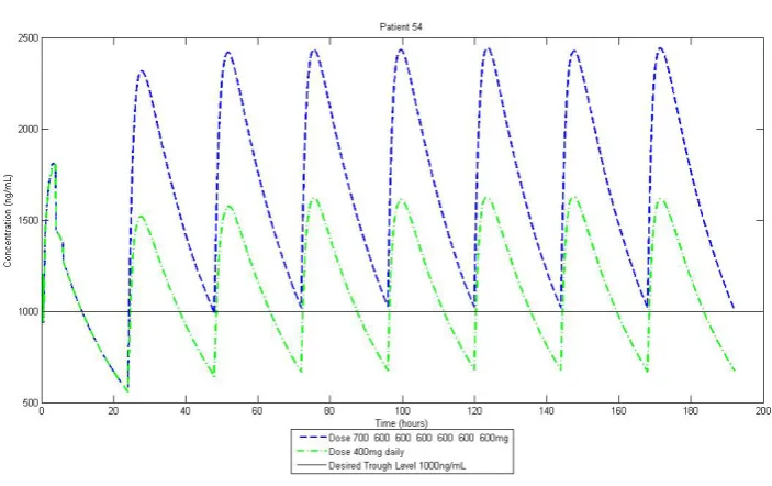
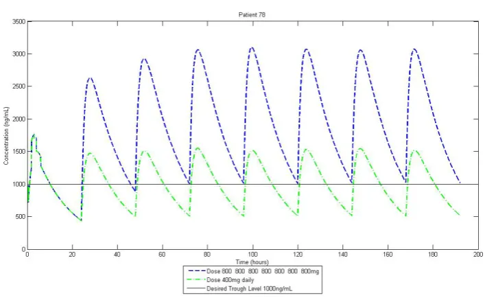
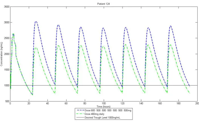
7 Stochastic Control with Pharmacodynamic Targets ___________________ 183 7.1 Example of Estimating an Optimal Dosage Regimen to Control a

Pharmacodynamic Response ____________________________________________ 183 7.1.1 Introduction __________________________________________________________ 183 7.1.2 Method ______________________________________________________________ 185 7.1.3 Results ______________________________________________________________ 192 7.1.4 Conclusions __________________________________________________________ 194

PREFACE

“At present you need to live the question. Perhaps you will gradually, without even noticing it, find yourself experiencing the answer, some distant day.”

Rainer Maria Rilke, Letters to a Young Poet.

I am sure my words lack ability to express the full extent of a rewarding experience that the research herein has provided, however, please accept this statistician’s attempt. My two supervisors Dr. Steven Lane and Dr. Andrea Jorgensen have been continual sources of motivation and support, I am sure that a better pair of mentors would be difficult to come by. I express my sincere gratitude to Professor Paula Williamson and Professor Munir Pirmohamed who both provided funding that allowed my studies to be possible. To Dr. Andrea Davies, Dr. Martin Smith and the members of the Laboratory of Applied Pharmacokinetics I express my thankfulness for your respective contributions to the research in this thesis.

To the department of Biostatistics I say thank you for providing an effective research environment and for always being there during the delights and pressures of the Ph.D. whether with a strategically placed coffee break or kind words.

DECLARATION

Work from Chapter 5 has been published in the following journals:

Francis B. DIA 2012 48th Annual Meeting Student Poster Abstracts. Drug Information Journal 2012; 46: 494-504.

The poster presentation ‘Using Stochastic Control Methods and Pharmacokinetics to Individualise Drug Therapy’ was awarded 2nd Place in The DIA 2012 Annual Meeting Student Poster Session.

1

INTRODUCTION

The following chapter contains background information on the motivation for the research conducted in this thesis. Particular attention is given to introducing individualised drug therapy and then explaining why it is important in healthcare.

In order to better treat the patient the stages of data collation to enable individualisation of drug therapy are explained. Following this, an explanation overviews the impact and reception of individualised drug dosing, highlighting the current level of research activity and with subsequent reasoning for this level.

1.1

The care of a patient involves effective diagnosis and treatment; during the treatment of a condition or disease the clinician will often prescribe some form of drug therapy. This drug treatment will aim to treat the ailment directly or indirectly by relieving one or all of the symptoms that are presented by the patient.

The list of drugs in healthcare used to treat various conditions and diseases is vast with new drugs added every year. Many drugs cause adverse events which are dose dependent, consequently there is a need to identify the correct dose for each specific patient, maximising the efficacy of the drug whilst minimising their risk of experiencing an adverse drug reaction (ADR).

the main objective of testing is to show an acceptable level of safety and efficacy in the general population. Most dose identification will be optimal for the ‘average patient’ and this is estimated from statistical analysis of the population using summary statistics such as the mean drug response.

The recent focus towards personalised medicine has highlighted this issue in drug dosing; the administration of the dose that is appropriate for the average patient will lead to a hugely variable response over the entire population. Identifying and measuring these sources of variability leads to drug dose algorithms which personalise drug therapy for the patient. The benefits of drug dose algorithms include more optimal treatment for the patient and the potential reduction in treatment costs from minimising the occurrence of adverse events.

1.2

The objective of a drug dose algorithm, to find the optimum dose, is complicated by the inter-individual variability in the response of each individual patient to a specific drug. Inter-individual variability is inherently biological due to each patient’s PK, what the body does to a drug, being unique. In a population of highly variable, in drug response, patients, patterns of variability must be identified.

patient has PK different from other patients; the modelling of this interplay is explained in Chapter 2 of this thesis.

Figure 1-1: Relationships of Sources of Variability Affecting the PKs of the Patient (Jamei et al., 2009).

The various relationships shown in Figure 1-1 and their effect on patient response will be more consequential for some drugs and nullified in others, for example, renal function will impact on clearance of all renally excreted drugs [2] whereas brain volume is only considered when drug molecules are small enough to enter the brain [3].

applied to the individualisation of a dosage regimen to aid clinicians in drug therapy decisions. Examples include linear regression methods in warfarin therapy [4], maximum a posteriori (MAP) Bayesian methods also in warfarin therapy [5] and stochastic control methods in digoxin [6]

Overall, the information for individualising a dosage regimen comes from many different sources. Identifying and measuring the variability that these sources cause in PK/PD response is important so that statistical methods can predict future PK/PD response of various patients in a population that require individualised dosage regimen to reach therapeutic targets. Often sources of variability are identified from specialised studies, such as clinical trials looking at the pharmacogenetics, the study of how genetic differences affect drug response. Gaining this information on variability from specialised studies means collaboration across disciplines is needed to incorporate the information effectively.

1.3

Often both sources of variability do not act in a linear way or act together to produce an enhanced effect on patient response to a drug. Understanding the magnitude of effect from the sources of variability is a requirement to facilitate individualise drug therapy. However, this understanding involves many different fields of medicine, which also relies upon effective collaboration. For example, to understand the effects of a patient’s genetics on drug response the expertise of a pharmacogenetic researcher is required, however, to then relay this expertise into a PK/PD model a pharmacometric researcher would be needed.

Figure 1-2: Flow Diagram of the Individualisation of Dosing.

The main focus of this thesis, the development of a drug dose algorithm, requires research into the magnitude of the variability caused by patient characteristics. Therefore the ability to estimate an individualised dose for a specific patient, currently, is only possible relatively late after a new drug is developed.

Figure 1-3 is taken from a publication highlighting the importance of genomically derived biomarkers by Meyer et al. (2002) [11]. Within the circle of Figure 1-3 there are phases of research that reveal sources of variability to individualise drug therapy. Moreover, Figure 1-3 shows research is conducted into the clinical targets for drug therapy, this research is a particular requirement to allow statistical methods to be utilised to individualise dosage regimens. For example, targeted studies confirm clinical PK/PD response targets that are used directly in algorithms as a mechanism to ‘judge’ dosage prospective dosage regimens; this will be explained further in Chapter 4.

Animal Modelling Biomarkers Target Study

Co-Morbidity Study

Co-Medication

Study Pharmacogenetics

Figure 1-3: Personalised medicine — integrating drug discovery and development through molecular medicine. Genomically derived biomarkers are being identified throughout the drug discovery and clinical development process. They will not only support personalized medicine, but will also enhance drug discovery and clinical development by generating new targets, validating targets and identifying patients that will benefit from novel therapeutics. ADMET, absorption, distribution, metabolism, elimination, toxicity [11].

The research in personalised medicine is shown in this section to be a connected network of various disciplines and areas of science. This research network seeks to improve the care of the individual patient by continual investigation of both intra- and inter-individual variability in patient response to drug therapy. This variability is then considered in statistical methodology to individualise dosage regimens that seek to bring a patient to therapeutic response.

1.4

Holford and Buclin (2012) [13] considered different levels of perceived variability of drug response and dosing methods available to create a criterion for dose individualisation. The different dosing types were population dosing (single dose for all patients), group dosing (different doses based on covariates) and target concentration intervention (doses estimated through monitoring measured drug responses) depending on the predictable and unpredictable variability seen in the drug response of the population. This thesis focuses on using stochastic control to achieve the latter type of individualised dosing.

Overall, when perceived variability complicates the estimation of an individualised dosage regimen stochastic control methodology has been used to guide a patient to therapeutic response. Firstly the system is individualised by predicting the response of the patient to different dosage amounts. Secondly, the vast information and research assimilated to aid the decision of individual dose is continually updated. And finally, when measurements are taken they are reconciled with the predictions made by the dose-exposure-response model to ensure variability around the patient response is reduced.

1.5

The uptake of sophisticated methods to achieve the goal of individualising drug therapy, such as stochastic control, has been limited despite their long time availability. To name but one, the Laboratory of Applied Pharmacokinetics (LAPK) has produced research based on stochastic control methods for over 20 years [17]. As highlighted in this chapter, research in this area has been limited by the need for collaboration between disciplines. The fusion of clinical expertise and statistical methodology needed for sources of variability to be correctly integrated into a drug dose algorithm is hard to attain. For large scale uptake of drug dose algorithms to occur collaborations need to be assembled internationally.

methodological research is undertaken that would appropriately harness the variability in pharmacology yet applicability is not fully considered; explained more in Chapter 4.

With these issues in consideration the reasons for the lack of drug dose algorithms being used in standard clinical practice is understandable. Yet, the advancements that could be achieved with further research must not be overlooked; already benefits have been shown such as in Jelliffe et al. (2012) [6] where an explanation is provided as to how digoxin therapy has been optimised for patients since the 1980s. To improve individualised drug therapy by better estimating the patient response and incorporating more clinical opinion, further research into applying stochastic control theory to individualising dosage regimens is presented in this thesis. In Chapters 5, 6, and 7 of this thesis examples will be given that demonstrate the applied methodology of the stochastic control approach explained in Chapter 4.

Chapter 5 will concentrate on estimating dosage regimens to induce a PK target. Initial applications will explain the stochastic control approach and introduce novel methodological research presented in this thesis. The final example of chapter, section 5.3, utilises the full stochastic control methodology proposed in section 4.3. The research of section 5.3 has been presented previously at the Drug Information Association 2012 conference and the Population Approach Group Europe 2012 conference and subsequently published as abstracts [18, 19].

therapeutic effect and an adverse event occurring. Section 6.4 explains the new methodology of incorporating a Markov model within the cost function to consider probabilities in dosage regimen estimation. The methodology is then applied to the imatinib example again to enable comparison of the dosage regimens estimated in section 6.5.

2

PHARMACOKINETICS AND PHARMACODYNAMICS

Chapter 1 introduced the paradigm of individualising dosage regimens prescribed to the patient. The PK/PD of a patient can be represented in a mathematical model, the study of pharmacometrics. From this model the response of the patient can be predicted and estimated for different dosage regimens.

This chapter begins with a brief explanation of the science that the PK/PD model is to represent, as well as an introduction to the objective of PK/PD models in translational medicine. With this background, the pharmacometric model is laid out including an explanation of the parameters within the model. Finally, approaches used in current software packages that calculate PK/PD parameters are explored.

2.1

2.1.1

PK is an umbrella term for many areas of research into the mechanisms of absorption and distribution of an administered drug, the chemical changes of the substance in the body and the effects and routes of elimination of the drug from the body. Overall, PK is the study of how the body affects an administered drug. The research areas in PK are condensed into the acronym ‘LADME’ that stands for:

In each area, there can be significant intra and inter-individual variability, due to this variability, the study of PKs is crucial in the determination of the appropriate dosing of a drug to a particular patient. To appropriately mimic patient PK, mathematical models are required that include parameters representative of the PK processes in the body. PK studies are necessary to determine by how much or why parameters vary between individuals.

PK is often studied along with PD, which is the study of how the drug affects the body. Both areas provide valuable information when investigating a drug’s possible effect both on a population of patients and/or an individual patient and as a consequence can inform individual dosage regimens, with the aim of increasing efficacy and reducing the risk of adverse events.

2.1.2

The study of what the drug does to the body is called PD. Examples of PD outputs include the intensity and duration of a drug’s therapeutic effect or an adverse drug reaction. The biology in PK refers to how much of a drug is at a site of effect in the body. PD studies investigate the effect that this amount of drug is generating by being at the site of effect, therefore PK is tandem to PD. PK/PD models will model the complete process from dose to drug effect (see section 2.2.5).

dependent variable (plasma concentration or clearance) of the drug in the body is not indicative of therapeutic effect [21], and thus warfarins PD response, measured in terms of the International Normalised Ratio (INR), is referred to instead to indicate a therapeutic effect.

2.1.3

Pharmacodynamics

The application of mathematical modelling to PK/PD, called pharmacometrics, allows models to be constructed to derive an estimate for PK/PD responses over a continuous time frame, such as the concentration of a drug in the plasma of the blood after an IV infusion. Pharmacometrics uses statistical techniques to estimate parameter values. The relationship between these parameters, the model, describes the time profile of a PK/PD response. The PK/PD model facilitates the ability to compare, evaluate and predict future PK/PD response.

To construct a combined PK/PD model the relationship between the concentration of drug in the body/plasma (the PK measurement) and the magnitude of the drug effect (the PD measurement) must be established. This link between the PK and PD varies in mathematical complexity, as will be explained in section 2.2.

2.1.4

PK data is variable in quantity; datasets can be sparsely or densely sampled. Densely sampled data tends to be difficult to obtain, this is due to the processes needed to measure the PK response. Sampling is normally done by taking blood through IV bolus or cannula and due to the invasive nature patients are often reluctant to consent to frequent sampling, hence sparse sampling is often undertaken. However, with fewer samples from a single patient often intra-individual patient variability is hard to quantify and this impacts on the certainty of subsequent parameter estimates of patient PK/PD.

2.2

2.2.1

When applying statistics to biological systems there is need to make assumptions to allow the construction of mathematical models that appropriately represent collected data. The assumptions are necessary because statistical models are more simplistic than biological systems that exist in our bodies [1]. However, although these models are more simplistic, the discrepancy between statistical models and actual biological systems need not be an issue when assumptions are properly handled.

For the construction of the models there are a number of mathematical techniques used to model PK/PD processes including, in order of diminishing complexity, physiology based, compartmental and non-compartmental models.

Predominantly physiology based modelling has only been used in PK application, physiologically-based PK (PBPK). For this modelling technique, anatomical and chemical pathways in the body are both considered individually in the model. For example, the anatomical pathway of blood flow between the spleen and portal vein [1].

Thirdly, non-compartmental models consider the concentration profile of a patient without time. Using this approach the concentration is not constrained to follow assumptions that are made in compartmental modelling.

The pharmacometrician must be aware of the trade-off between simplified and complex modelling. Simplified modelling will bring benefits such as easier comprehension, less computational requirements and reduced mathematical complexity whereas more complex modelling may lead to greater accuracy in predicting a PK process [1, 22].

To allow the methodology to be explained thoroughly, in this thesis, compartmental modelling will be utilised. Compartmental modelling is preferable as it has been the standard modelling technique in pharmacometrics for over forty years [23]. Further, compartmental modelling involves significantly less mathematical formulae than PBPK modelling; this allows for more complex control methods, explained later in the thesis. With concentration-time sensitive responses being considered this thesis, such as an adverse event caused by a drug concentration above a certain value in time, non-compartmental modelling would not be appropriate as time is not considered in these models.

2.2.2

liquid to flow differently. This system of boxes provides a crude parallel with the body’s PK/PD system as a drug moves across tissue membranes within the body.

Each box represents a different aspect of the body’s pharmacology; an area commonly represented in PK applications is the central plasma compartment where the concentration of the drug in the plasma of blood (the ‘plasma concentration’) at the site of drug action is considered.

The flow rates between boxes describe the drug concentration being distributed around the body or excreted out of the body. The flow rate can be as simple as a unit amount of drug per hour up to more complex systems like those described by Michaelis-Menten kinetics [24]. More boxes and complex absorption rates lead to more PK/PD parameters to estimate, shown in section 2.2.4.

Compartmental modelling seeks to describe the PK/PDs of the body in a more simplistic way to the actual bodily processes. Due to this, PK/PD data from different studies of the same drug may be modelled differently; in two publications regarding the PK of warfarin by Hamberg et al. (2007 & 2010) [21, 25] two different models were used. This difference in models can occur due to a number of factors including different sampling frequencies in the data, assay errors of measurements and the different inter-individual variabilities seen in the two derivation cohorts.

multi-chain compartments designed to model various phases of drug effect. PD models will be discussed further in section 2.2.5.

2.2.3

Although compartmental modelling is a simplification of the biological processes seen in the body, the parameters used in modelling can still be interpreted physiologically. This is important as patient characteristics can be drawn from specific parameter values, for example, lower than normal parameter values for a patient’s elimination of a drug could indicate deteriorating condition. Parameter values can be calculated for either a population (population mean) or an individual patient (patient-specific mean) along with their respective variances.

The PK parameters for absorption can range from a single constant to more complex absorption rates involving several parameters. For oral dosing, the standard modelling technique is to use an absorption compartment which acts to gradually release the drug into the blood, this mimics the gastrointestinal tract [26]. Whereas with intravenous infusion the release is considered instantaneous as the drug immediately enters the blood stream [27]. In the simple case for oral dosing the PK parameter, the rate constant of absorption, denoted is used. The rate constant of absorption describes the rate the drug enters the apparent site of interest, e.g. plasma concentration of a drug in the plasma of the blood.

depending on the complexity of the distribution model. The parameter is theoretical in the sense that the volume of distribution is the amount of volume that the drug would have to equilibrate over in order to derive similar concentrations of drug in the plasma. Whilst the name suggests a quantity of space, the parameter considers elements such as solubility and size of the drug molecules. Drugs that have a larger molecule size will have a smaller volume of distribution to the drugs with smaller molecule size due to distribution across different tissue membranes [28]. The drug in the blood is assumed to instantaneously mix over the entire volume of a compartment, for example, it would be assumed that blood samples from two different areas of a compartment would contain the same concentration of the drug.

Elimination is the rate the drug is excreted from the body over time. In the simplest case, three parameters contribute to this phase of PK, the volume of distribution, , the clearance denoted , and the constant of elimination denoted . The clearance is the amount of blood that has drug extracted from it

over time. These elimination parameters are proportional through the volume of distribution with a linear relationship described as such,

2.1

These parameters are used in models to construct a relationship that derives the concentration, , of a drug in a compartment or compartments. The different ways

2.2.4

Different drugs will have different systems of PK parameters as the body processes the drugs in different ways. PK/PD models can parallel bodily processes sufficiently to generate acceptable predictions that coincide with measurements taken from a patient, such as, plasma concentrations of a drug measured from blood samples. The predictive power of a model is determined by how close estimations are to measurements.

Pathways of administration are drug formulation specific. Different pathways of administration include constant intravascular (IV) infusion over a certain duration of time, IV bolus and oral dosing. Each pathway of administration needs to be treated differently when modelling. With IV routes of administration it is assumed that the drug is instantaneously absorbed into systemic circulation [29]; whereas with oral dosing the absorption process is not instantaneous and so there is a need to calculate the appropriate absorption PK parameters.

Figure 2-1: Concentration-Time Plots for Different Routes of Drug Administration in a One Compartment PK Model.

and IV bolus doses. This is due to the drug being gradually released into the central plasma compartment through gradual absorption. To model this gradual absorption an extra compartment is needed; in this extra compartment the oral dose instantaneously appears and is released at the desired rate into the central plasma compartment. With IV infusion and IV bolus routes it is assumed that the drug instantaneously enters the central compartment thus the concentration curves are declining once the drug enters the compartment.

The three curves in Figure 2-1 are derived from a one compartment PK model. A one compartment model assumes that the entire area of distribution in the body is one rapidly mixed compartment where the drug flows around constantly and is not subject to different rates of flow. This model is applied to various drugs [30, 31].

Figure 2-2: Graphical Representation of the One Compartment Model.

The one compartment PK models for IV infusion (equation 2.2), IV bolus (equation 2.3) and oral dose (equation 2.4) are parameterised as

_{( )}

( _{) 2.3}

( ) ( ) 2.4

where is the infusion rate given during the time interval ( ), is an

IV bolus dose given at time , is an oral dose given at time .

Some drugs, such as vancomycin [32], are better modelled with a two compartment PK model. The concentration time curve will display a two stage elimination when the drug has to travel through different mediums of tissue in the body leading to some of the drug being distributed quickly and the remainder distributing more slowly [33]. To model the different phases of elimination, an extra compartment is added to the model, the ‘peripheral compartment’ which has two pathways one in and one out of the central compartment.

Figure 2-4: Graphical Representation of the Two Compartment Model.

The two compartment PK models for IV infusion (equation 2.5), IV bolus (equation 2.6) and oral dose (equation 2.7) are described mathematically as:

( )((

) ( )₎

( ) ( _{) )}

2.5

( ( )

( )( )

( )

( )( )

( )

( )( ) )

2.7

where (( ) √( ) ) formulated

in Metzler et al. (1971) [34] includes parameters and that represent the

flow rates into and out of the central plasma compartment, .

Models can be extended to more than the one and two compartmental models discussed above by adding compartments to describe different PK processes until the model represents the complete physiology of the patient; this is the methodology of PBPK modelling [1]. With PBPK intricate and precise processes will be mathematically described leading to individual pathways and organs being described with their own flow rates and compartments.

2.2.5

The process of linking the PK of a drug to the PD in modelling begins by interpreting the concentration of the drug in the central compartment as a magnitude of effect that then occurs as a consequence. For instance, a model for warfarin would link the concentration in the plasma to the consequential anticoagulation effect of the drug. Often, there is a delay in a patient experiencing a therapeutic drug effect after a target drug exposure is attained [35]; this delay is modelled by adding one or more compartments to the PK model. The Hill equation is one of several models used to interpret the concentration of the drug in the central compartment as a value of drug effect [36].

2.8

where is the effect of a drug at time . is the baseline effect on the

body in absence of the drug, for example an INR value of 1 before warfarin is prescribed [21]. If there is no baseline effect level in the body in the absence of a drug then is equal to zero, this occurs in drugs that cause effects that

naturally the body wouldn’t exhibit, for example, muscle relaxation and altered central nervous system function [37, 38]. The maximal effect that the drug can cause to the body is described by the parameter . The parameter is the

Figure 2-5: Graphical Representation of the Two Compartment PK Model with an Effect Compartment.

(

) 2.9

equation to describe the effect compartment is given in equation 2.9. To describe the entire model in Figure 2-5 mathematically equations 2.6, 2.7 and 2.9 are used.

The PD model described in this section can be used to describe various drug effects. For example, later in this thesis, the PD effects of imatinib and simvastatin will be considered with the above model. Imatinib is a drug used to treat leukaemia by encouraging cytogenetic and molecular effects in the body [39], whilst simvastatin is dosed to reduce a patient’s cholesterol levels in a desired target [40].

2.3

As shown in section 2.2, PK/PD model consist of parameters that describe internal processes, e.g. the absorption of a drug from the gut. Due to the multiple parameters involved in PK/PD model particular software is required to analyse data. PK/PD data is analysed to estimate values of parameters however different methods and assumptions are used by software packages. One particular difference in methodology regarding the estimation of individual parameters is important due to the derived distributions. The different methodologies parametric and non-parametric are discussed briefly in the next two sections.

2.3.1

The NONMEM software is a program that performs regression analysis and in particular is able to perform non-linear regression. As parameters within PK/PD models are random variables, distributions of these random variables require particular estimation methods. The parameter estimation methods included in NONMEM, such as conditional likelihood and Laplace transforms, mean parametric distributions can be calculated for parameters.

NONMEM includes fixed effects in models as population values of parameters then random effects represent the between subject variability. Both of these values are assumed to be represented by a parametric distribution. The combination of these two effects into a mixed-effect model allows individual parameter distributions for each patient. For example an individual’s clearance is expressed as

̂

2.10

where is the typical (population) value, ̂ is a random effect quantity for an

individual. This relationship leads to a being a log-normally distributed individual

parameter distribution which is appropriate as pharmacometric parameters tend to follow this behaviour [42] and a property of the distribution is restriction to non-negative values. This is important as PK parameters are assumed non-non-negative biological values.

2.3.2

perform parametric and non-parametric analysis however both packages retain their respective main approaches of parametric and non-parametric analysis.

With a non-parametric approach, the models for a patient’s PK/PD remain however the parameters in the models are not assumed to follow a distribution such as log-normal. The basic intention is to allow the data to determine the shape of the distribution. As the distribution is purely determined from empirical data and not altered by a parametric assumption the statistical property of consistency is assured. As more data is collected the distribution of the parameters will approach the true distribution of the parameters.

Figure 2-6: The Comparison of Non-Parametric and Parametric Analyses (Neely et al. (2012)).

“A, Results of the NPAG fit. True parameter values from the simulated population are shown as black squares, with NPAG support points shown as circles whose size is an approximate multiple of the size of 1 square, proportionally increased according to the probability of each NPAG point.

B, Results of the IT2B fit. True parameter values are shown as white squares. Note the outlier in the upper right corner. The bivariate normal parameter distribution estimated by IT2B is depicted as ellipses of fading colour corresponding to the percentile of the distribution. The white cross at the centre is the mean.”

In the top right of A and B in Figure 2-6 there is an outlying set of parameters, it is clear that whilst the non-parametric analysis (A) attributes probability to this point, the parametric approach (B) does not do so. Secondly, the parametric approach used in B, has the ability to define a bimodal distribution. A bimodal distribution would potentially be more appropriate for this data but analysis does not conclude a bi-modal distribution, rather the two ‘strands’ of parameter sets are combined into a unimodal distribution in B.

3

ASSESSMENT OF A DRUG DOSE ALGORITHM NOT INFORMED

Drug dose algorithms are effective when they capture a high amount of inter-individual variability in the population. However, often a large amount of data is needed to identify sources of variability but the required data can be hard to obtain.

In view of this challenge, a large amount of research has been conducted that does not require invasive data such as plasma concentrations. In this chapter, methodology outside the main focus of this thesis, stochastic control methods, is presented. A commonly utilised method, the linear regression algorithm, is presented as a worked case study in warfarin. In comparison to other methods the application of a linear regression algorithm requires reduced computational demand and data which is easier to obtain, such as the demographic factor, age.

3.1

3.1.1

Warfarin is the most commonly used anticoagulant in the UK, with an estimated 1% of the population currently undergoing warfarin therapy [44]. The aim of warfarin therapy is to bring INR, a measure of the patient’s clotting capability, within a therapeutic range, and to maintain it within that range. Although warfarin is an effective anticoagulant, determining the dose required to achieve a stable therapeutic INR (the ‘stable maintenance dose’) is difficult due to the large inter-individual variability in maintenance dose requirements, and warfarin’s narrow therapeutic index.

The therapeutic INR range is typically 2 to 3 for warfarin patients, and outside this range adverse events are more likely to occur [45]. If the concentration of warfarin in the body is too low then the drug will not provide desired therapeutic effects, leading to a risk of thrombosis. Conversely, if the amount of warfarin in the body is too high there is an increased risk of the most critical adverse event associated with warfarin therapy, severe haemorrhage [44]. In a recent large study of reasons for hospital admissions in the Merseyside, England, warfarin was shown to be the third highest cause of an ADR, being responsible for just over 10% of all hospital admissions for adverse drug reactions [46].

include, with some including only patient demographics such as age, weight, height and co-morbidities, others including details of initial INR measurements and loading doses and others including details of co-medication with drugs known to alter the effect of warfarin. Models comprising only demographic, loading dose or co-medication details use information that is readily available to the clinician and a few recent studies have derived such algorithms [47, 48].

More recently, to explain more variability in individual maintenance dose requirements, dosing algorithms have also included genetic factors [4, 49-52], in particular variants in the VKORC1 and CYP2C9 genes. These genes have been identified in pharmacogenetic studies to be consequential in dosing requirements due to their effects on PK/PD [53]. However, the benefit of including genetic information in dose prediction remains to be shown in practice [54, 55] despite the science being conclusive that a patient’s genetics alter their warfarin dose requirements [44, 53].

When developing dose prediction regression models, the outcome of interest is stable maintenance dose; therefore it is necessary to identify, for each patient included in the dataset used to derive the model (the ‘derivation dataset’), the dose at which stable, in-range INR has been achieved. However, since INR is sensitive to many factors, including dietary changes [56] and alcohol intake [51], measurements often fluctuate out of range even after an initial period of stability has been achieved.

(INR 2-3). Thus, defining what constitutes a patient’s stable maintenance dose is difficult and importantly this dose may change over time.

The top graph for patient 1 demonstrates an example of a patient with highly fluctuating INR level. At some points the dosage amount of 6mg appears to induce an in-range INR value however at other times it is not sufficient for efficacious effect. For patients such as this constant monitoring and appropriate dosage regimen adjustment is recommended to ensure maximal warfarin therapy. Unfortunately, linear regression methods are non-adaptive to patient response and such dosage adjustment is only possible if particular covariates are included. For example, if an INR measurement on a certain day after therapy initiation was included as a covariate.

The middle graph shows patient 4 on a constant dose who remains within the therapeutic range for the duration of the study. With a drug such as warfarin this is a rare occurrence; however the patient’s INR curve does move very close to the minimum and maximum target INR values on two occasions. These small divergences could be due to demographic changes such as weight fluctuations, dietary factors or co-medications that cause only slight effects on the efficacy of warfarin. Linear regression methodology does not permit effective modelling of small divergences as parameters are assumed constant.

Patient 26 is a clear example of variability that maintenance dosing algorithms do not incorporate as the patient has not been induced to a constant in-range INR level. Linear regression methods use a process of patient selection through steady state criteria to build a dataset for dose algorithm derivation. This process could be seen as a ‘cherry picking’ process where patients whose dosage regimen does not cause a constant in-range INR, potentially entire outlying populations of patients, are excluded from the dataset. These outlier patients are exactly those who require accurate dosage regimen estimation the most.

Despite the number of published dose prediction regression models, they have rarely been integrated into standard clinical practice [54]. This, in part, is due to the fact that most of these algorithms have not been externally validated in an independent dataset and if they have then replication has been poor [10, 57, 58]. With a view to assessing how well previously published models predicted dose in a dataset outside the derivation dataset, their predictive ability was tested in an independent patient cohort. This also allowed the performance of the models to be compared against each other. Further, it allowed the evaluation of how suitable linear regression, the most commonly utilized method for deriving warfarin dosing algorithms, is to estimate maintenance dosing; particularly in light of the fact that the stable dose for a patient can change with time.

3.1.2

Table 3-1:Demographic, Clinical and Pharmacogenetic Information of Patients in the Validation Cohort.

Variable Patient Data

Number of Patients 508

Age Mean 68 (SD 13)

Gender Male: 280 (55%) Female: 228 (45%)

Weight (kg) 82 (SD 19)

Height (cm) 169 (SD 11)

Therapeutic dose (mg) 4.19 (SD 2.05)

On Amiodarone Co-medication Yes- 46 (9%) No- 462 (91%)

CYP 2C9 \ *1 *2 *3

*1 313 98 43

*2 4 9

*3 3

VKORC1 GG GA AA

206 224 77

SD: Standard Deviation

In the Liverpool study, a stable maintenance dose was defined as the daily dose required to achieve three consecutive INR measurements within the individual’s target range (2-3 unless patient required a different therapeutic range). A stable maintenance dose was identified on the assumption that patients fully complied with their dosing regimens and that the only reason for dose modification was recorded clinical practice. After applying this definition of stable maintenance dose, of the initial 997 patients, 508 patients were found to have achieved stability during follow-up and they formed the subset of patients included in the ‘validation cohort’.

not considered from publications over ten years old which meant that the majority incorporated pharmacogenetic information [53]. Variables included in the models included a unique combination of any of the following types demographic, clinical, pharmacogenetic, and dose response and co-morbidity information. Applicability to the validation cohort was mandatory; this meant models selected would need to consist of covariates measured in the Liverpool study. The models’ initial performance in the derivation dataset was also highly important, on the basis that algorithms tend to predict less of the variability in validation datasets [10, 58]. The search for dose regression models was conducted on the 20th of December 2011.

3.1.2.1 Statistical analysis

To determine the ability of the regression models to explain variability in dose requirements in the validation cohort the warfarin dose predicted by the regression model was plotted against the actual warfarin dose and then a linear regression line fitted. The accuracy of the algorithms was judged using the R-squared statistic (unadjusted and adjusted), mean absolute error (MAE), mean percentage absolute error, and the slope and intercept of the regression line.

The mean absolute error (MAE) statistic measures how close the predictions are to the actual values across all patients in a dataset, and therefore is important when considering which model has the best predictive capability. However, the clinically desired value of this statistic varies. For example, in an opinion publication Kimmel [59] recommended a MAE of 1mg/day because ‘a change in warfarin dose from a baseline of 5mg is sufficient to change the INR by 0.5’.

The slope and intercept of the R-squared line are also measures of a model’s accuracy, a slope of one and an intercept of zero indicate that there is no proportional or constant error respectively. If the slope coefficient is different from one there will be either over or under prediction in some, if not all estimated doses. The intercept term gives an insight into how well the model is predicting at low doses. These statistics should all be used together to appropriately judge a model as each statistic can appropriately assess a different aspect of the model’s predictive ability.

3.1.3

Table 3-2:List of dose prediction models [4, 47-50, 60].

1. Was the paper published after 2002?

2. Does the model contain more than two different covariates than another dose prediction regression model already selected? (Although, where relevant novelty existed similar dose prediction regression models were compared and this novelty explained.)

3. Does the model include only covariates measured in the Liverpool study?

4. As R-squared is the most frequently reported statistic to judge model performance in the reviewed papers, is the value of this statistic above 0.5?

*R-squared statistic from derivation dataset not reported.

#Reason for inclusion explained in manuscript.

The model presented by Le Gal et al [48] includes only clinical covariates, including INR measurements on day 5 and day 8 and the total dose of warfarin taken during the first week. The second model, proposed by Solomon et al [47] includes

Paper Dosing Equation 1 2 3 4

Le Gal et al. ln(Dose) = 2.5 + 0.1*(Total first week dose)

– INR at day 8 + 1.5*(INR at day 5 <2.0)

2009 Y Y 0.88

Solomon et al. Dose = 3.26 – 0.31*(amiodarone) – 0.032*(age)

+ 0.28*(Loading Dose/end of load INR)

2004 Y Y 0.80

Anderson et al. Weekly Dose = 1.64 + exp[3.984 – 0.197*(*1*2)

– 0.360*(*1*3) – 0.947*(*2*3) – 0.265*(*2*2)

– 1.892*(*3*3) – 0.304*(VKORC1 CT)

– 0.569*(VKORC1 TT) – 0.009*(age) +0.094*(gender)

+ 0.003*(weight)]

(25% dose reduction for those on amiodarone)

2007 Y Y U*

Wadelius et al. √(Weekly Dose) = 9.46832 – 0.90112*(VKORC1 AG)

– 2.01863*(VKORC1 AA) – 0.50836*(CYP2C9 *1*2)

– 0.97546*(CYP2C9 *1*3) – 1.10204*(CYP2C9 *2*2)

– 1.74761*(CYP2C9 *2*3) – 3.40061*(CYP2C9 *3*3)

– 0.036868*(age) – 0.27698*(female)

– 0.06992*(# of drugs which increase INR)

2008 Y Y 0.59

Sconce et al. √(Dose) = 0.628 – 0.0135*(age) – 0.240*(CYP*2)

– 0.370*(CYP*3) – 0.241*(VKOR) + 0.0162*(height)

2005 Y Y 0.54

Zhu et al. ln(Dose) = 1.35 – 0.008*(age) + 0.116*(gender)

+ 0.004*(weight) – 0.376*(VKORC1-AA)

– 0.318*(2C9_3) + 0.271*(VKORC1-GG) – 0.307*(2C9_2)

information on total loading dose, INR at the end of the loading phase, age and the use of the co-medication amiodarone. The drug amiodarone inhibits the clearance of warfarin meaning that patients taking it should be prescribed a reduced dose of warfarin. These two models do not include any information on genotypes and, as a consequence, may have an advantage in that they are based on data readily available to the clinician, so can be used without having to attain a patient’s genotype information.

Four of the included models include genotypes for variants in CYP2C9 and VKORC1. The models proposed by Anderson et al. (2007) [4] and Wadelius et al. (2009) [60] assume that CYP2C9 alleles are non-proportional, thus including a separate covariate for each possible genotype, whereas the models proposed by Sconce and Zhu assume an additive effect of the variant allele.

The models proposed by Anderson et al. (2007) [4] and Wadelius et al. (2009) [60] calculate a total weekly dose of warfarin; consequently clinicians would have to divide the recommended weekly dose into seven daily doses as they consider appropriate.

The model proposed by Sconce et al. (2004) [47] included fewer covariates than most of the other pharmacogenetic models, with demographic information only on age and height being included along with information on the genotypes. Similar in composition, but including weight instead of height, the model derived by Zhu et al. (2007) [49] has already been externally validated once in the recent study by Linder et al. (2009) [58], and was found to explain slightly less variability in the validation dataset than in the derivation dataset. The reason for the inclusion of two similar dosing equations was to assess whether the model developed by Sconce et al. (2005) [50] derived at the University of Newcastle, United Kingdom has an advantage over models derived in other countries in explaining variability in the Liverpool-based validation cohort. Similarities could be evident in, for example, demographics and the ethnical constitutions of the two cohorts. The strength of these two models in particular was that they contain a small number of covariates yet explain a large amount of variability in their respective derivation datasets.

3.1.3.1 Dose Prediction Model Performance

Figure 3-2:Graphs of clinically guided predicted dose and actual warfarin dose.

Table 3-3:Table showing summary statistics about the performance of the six dose prediction models.

Model Absolute Error R-squared (%) Intercept Slope

(Error) Mean ± SD

(Percentage) Mean ± SD

Coefficient of Determination

Adjusted

Solomon 1.21 ± 1.23 36.3 ± 60.0 34.9 34.0 2.06 0.48

Le Gal 1.20 ± 1.31 39.3 ± 73.4 39.2 38.8 1.47 0.60

Anderson 1.16 ± 0.99 39.5 ± 68.6 41.4 40.6 2.71 0.45

Zhu 1.29 ± 1.34 32.6 ± 46.0 38.8 38.1 2.02 0.30

Sconce 1.28 ± 1.28 38.1 ± 64.5 29.5 28.8 2.41 0.38

Wadelius 1.46 ± 1.28 51.0 ± 88.5 35.6 35.0 3.15 0.46

From Figure 3-2 it can be seen that the Le Gal et al. (2010) model has predicted negative doses for some of the study participants. The reason why these patients were estimated as requiring a negative warfarin maintenance dose was a high INR or low dosages during the first week of treatment. The model does not have the ability to deal with these events and consequently the predicted doses for these patients are not applicable. To further investigate the model’s ability all negative warfarin dose estimations were set to zero, with this change the percentage of variability explained improved to 46.2%.

3.1.4

a therapeutic INR range. Further, if clinical endpoints are improved this often means the cost of therapy reduces [20, 61].

There is little doubt that pharmacogenetics can greatly inform warfarin treatment and this has been recognised with the updated recommendations on warfarin packaging by the United States Food and Drug Administration [62]. Further, a recent paper by Schwab et al. (2011) [63] declared the goals to achieve optimal complex, patient-dependent dosing regimens was to inform clinicians of pharmacogenetic principles and to build up health care teams.

Several warfarin dosing algorithms have been published, many including pharmacogenetic information, and the majority are in the form of linear regression models. In this chapter, six different dose prediction linear regression models were compared using an independent cohort of patients to test their predictive ability outside their original derivation cohorts. This was done by re-fitting each model in turn to the validation dataset and assessing the variability explained (R2), as well as comparing the predicted stable dose against actual stable dose. Acknowledgement is required that, unlike randomized control trials, this method of validation does not allow for dose prediction models to be assessed by clinical endpoints, for example time spent within therapeutic range as patients are not prescribed the dose predicted.

endpoints. However, several large, well powered trials are currently underway to investigate clinical endpoints further [67-69].

Unsurprisingly, the performance of all six models was worse in the validation cohort as compared to the derivation cohort [10, 58]. Although the diminished performance could be explained by several factors, this poor replication has also been observed previously [10, 51], leads us to hypothesise that regression modelling may not be the most optimal approach for developing a warfarin dosing algorithm.

A key reason for this is the fact that developing a regression model necessitates each patient’s stable maintenance dose to be determined in accordance with a particular definition of stable dose. Choosing this definition in itself is difficult as evidenced by the many different definitions given in the literature (see Section S2, Supplementary Appendix 1 [70]), and stable dose of a patient under one definition may well be different to the patient’s stable dose under another. Further, depending on the definition used, some patients are excluded from analysis on the basis that their dosing history never meets the criteria specified in the definition.

dose prediction regression models can overlook information needed to appropriately recommend doses for the least stable patients – exactly the patients who need individualized dosing.

All six dose prediction regression models, including two non-pharmacogenetic models, have performed at similar levels in this chapter. Based on these findings, it is stipulated that linear regression models may not be able to fully draw on the variability that pharmacogenetics can explain.

The need to exclude non-stable patients, the lower than clinically desired performance and apparent low ability to incorporate pharmacogenetic information [54, 59, 65, 66] of the linear regression dose prediction models validated here suggest that more advanced methods may be required for dose estimation. Methods such as those implemented in Hamberg et al. (2010) [21] and Perlstein et al. (2011) [71] incorporate non-stable patients into the analysis as well as looking at PK/PD parameters.

It must be noted, however, that models used to represent PK/PD are complex and therefore their implementation into clinical practice involve a large degree of collaboration. Dosing algorithms must be convenient and applicable to a practising clinician. In consideration of this, potential presentation solutions have been constructed, for example, the dose advisor made available through the internet

(www.warfarindosing.org), an Excel spreadsheet warfarin dose calculator [52, 70],

however this calculator’s algorithm are based on linear regression models. Alternatively, a table of recommended doses given in Hamberg et al. (2010) [21] generated by simulation from a PK/PD model. The potential solutions given are effective as initial dose recommendations, however if the patient does not respond to the recommended dose they offer no adaptive solutions.