Nonnegative Matrix Analysis for Data
Clustering and Compression
THESIS SUBMITTED
IN ACCORDANCE WITH THE REQUIREMENTS OF
THE UNIVERSITY OF LIVERPOOL
FOR THE DEGREE OF
DOCTOR IN PHILOSOPHY
BY
Liyun Gong
Department of Electrical Engineering and Electronics
The University of Liverpool
Liverpool, United Kingdom
Abstract
Nonnegative matrix factorization (NMF) has becoming an increasingly popular data
processing tool these years, widely used by various communities including computer
vision, text mining and bioinformatics. It is able to approximate each data sample in
a data collection by a linear combination of a set of nonnegative basis vectors weighted
by nonnegative weights. This often enables meaningful interpretation of the data,
mo-tivates useful insights and facilitates tasks such as data compression, clustering and
classification. These subsequently lead to various active roles of NMF in data analysis,
e.g., dimensionality reduction tool [11, 75], clustering tool[94, 82, 13, 39], feature engine
[40], source separation tool [38], etc.
Different methods based on NMF are proposed in this thesis: The modification of
k-means clustering is chosen as one of the initialisation methods for NMF. Experimental
results demonstrate the excellence of this method with improved compression
perfor-mance. Independent principal component analysis (IPCA) which combines the
advan-tage of both principal component analysis (PCA) and independent component analysis
(ICA) has been chosen as the significant initialisation method for NMF with improved
clustering accuracy. We have proposed the new evolutionary optimization strategy for
NMF driven by three proposed update schemes in the solution space, saying NMF
rule (or original movement), firefly rule (or beta movement) and survival of the fittest
rule (or best movement). This proposed update strategy facilitates both the clustering
and compression problems by using the different system objective functions that make
use of the clustering and compression quality measurements. A hybrid initialisation
approach is used by including the state-of-the-art NMF initialization methods as seed
knowledge to increase the rate of convergence. There is no limitation for the number
and the type of the initialization methods used for the proposed optimisation approach.
Numerous computer experiments using the benchmark datasets verify the theoretical
results, make comparisons among the techniques in measures of clustering/compression
accuracy. Experimental results demonstrate the excellence of these methods with
im-proved clustering/compression performance.
In the application of EEG dataset, we employed several standard algorithms to provide
clustering on preprocessed EEG data. We also explored ensemble clustering to obtain
firstly, normalization is necessary for this EEG brain dataset to obtain reasonable
clus-tering; secondly, k-means, k-medoids and HC-Ward provide relatively better clustering
results; thirdly, ensemble clustering enables us to tune the tightness of the clusters so
Contents
Abstract i
Contents v
List of Figures xi
Acknowledgement xii
Nomenclature xiv
1 Introduction 1
1.1 Motivation and Objectives . . . 1
1.2 Original Contribution . . . 2
1.3 Publications . . . 3
2 Clustering Analysis 5 2.1 Machine Learning . . . 5
2.2 Clustering Algorithms . . . 7
2.2.1 Problem setting . . . 8
2.2.2 Popular Clustering Algorithms . . . 10
2.2.3 Fuzzy clustering . . . 13
2.2.4 Kernel-based clustering . . . 14
2.2.5 Self Organizing Clustering . . . 15
2.2.6 Self Splitting and Merging Clustering . . . 17
2.2.7 Ensemble Consensus Clustering . . . 18
2.3 Clustering validation . . . 20
2.3.1 Internal Evaluation . . . 20
2.3.2 External Evaluation . . . 22
2.4 Summary . . . 24
3 Nonnegative Matrix Factorization 25 3.1 Introduction . . . 25
3.2.1 Multiplicative update rule . . . 27
3.2.2 Other update rules . . . 28
3.3 NMF Initialization . . . 29
3.3.1 Random initialization . . . 29
3.3.2 Cluster-based Initialization . . . 30
3.3.3 Dimensionality reduction-based initialization . . . 34
3.3.3.1 Standard Dimensionality Reduction Methods . . . 34
3.3.3.2 PCA and ICA based Initialization . . . 38
3.3.4 Why initialization . . . 40
3.4 Summary . . . 41
4 Proposed NMF Initialization Strategy 42 4.1 Introduction . . . 42
4.2 Clustering Based Initialization . . . 43
4.2.1 Method . . . 44
4.2.2 Results . . . 44
4.2.3 Conclusion . . . 53
4.3 Dimensionality Reduction Based Initialization . . . 54
4.3.1 IPCA Based NMF . . . 54
4.3.2 Results . . . 55
4.3.3 Conclusion . . . 66
5 Proposed NMF Updating Strategy for Data Clustering 68 5.1 Introduction . . . 68
5.2 Proposed Method . . . 69
5.2.1 Seed Matrix Generation . . . 69
5.2.2 Evolving Strategy . . . 70
5.2.2.1 Multiplicative rule . . . 70
5.2.2.2 Firefly Rule . . . 70
5.2.2.3 Survival of the Fittest Rule . . . 73
5.2.3 Score Function . . . 74
5.3 Experimental results and analysis . . . 74
5.3.1 Experimental Setup . . . 75
5.3.2 Results and Analysis . . . 76
5.4 Conclusion . . . 87
6 Proposed NMF Updating Strategy for Data Compression 89 6.1 Introduction . . . 89
6.2 Proposed evolutionary optimization strategy on data compression . . . . 91
6.2.2 Beta movement forW . . . 94
6.2.3 Best movement for W . . . 94
6.2.4 Objective function . . . 96
6.3 Experimental results and analysis . . . 97
6.3.1 Datasets and preprocessing . . . 97
6.3.2 Experiment process . . . 97
6.3.3 Yale image dataset . . . 98
6.3.4 ORL image dataset . . . 105
6.4 Conclusions . . . 112
7 Application of EEG Dataset 117 7.1 Introduction . . . 117
7.2 Clustering methods . . . 117
7.3 Experimental Results . . . 118
7.3.1 EEG data structure . . . 118
7.3.2 Results . . . 119
7.4 Conclusions . . . 133
8 Summary 134 8.1 Summary and conclusions . . . 134
8.2 Future Works . . . 135
List of Figures
2.1 The single linkage (nearest neighbour) distance), from [30] . . . 12
2.2 The complete linkage distance, from [30] . . . 12
2.3 The average linkage distance, from [30] . . . 13
3.1 Description of NMF and SVD basis vectors on face dataset, from [23] . 26
3.2 Error using different initializations, from [122] . . . 32
3.3 Comparison of initialisation methods in terms of sparsity and
orthogo-nality. (a) Comparison of initialisation methods in term of orthogonality
and (b) Comparison of initialisation methods in term of sparsity . . . . 33
3.4 Comparison of initialisation methods in terms of error . . . 33
3.5 Prostate cancer study: sample representation using the first two or three
components from PCA, ICA and IPCA, from [118] . . . 38
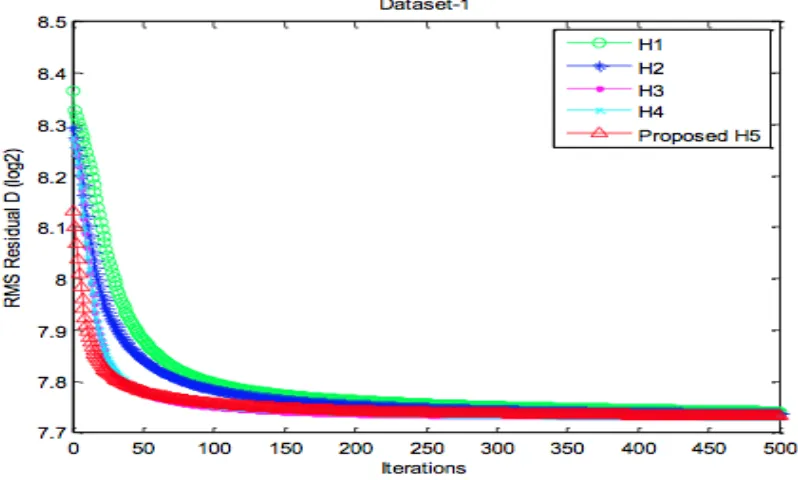
4.1 The average D log values of each of the five initialization methods
(Dataset 1) . . . 47
4.2 The average D log values of each of the five initialization methods
(Dataset 2) . . . 48
4.3 The average D log values of each of the five initialization methods
(Dataset 3) . . . 48
4.4 The average D log values of each of the five initialization methods
(Dataset 4) . . . 49
4.5 The average D log values of each of the five initialization methods
(Dataset 5) . . . 49
4.6 The average D log values of each of the five initialization methods
(Dataset 6) . . . 50
4.7 The average D log values of each of the five initialization methods
(Dataset 7) . . . 50
4.8 The average D log values of each of the five initialization methods
(Dataset 8) . . . 51
4.9 The averageD values of each of the five initialization methods with the
4.10 The average D values of each of the five initialization methods with the
increasing dimensionality number on Dataset 5-8 . . . 53
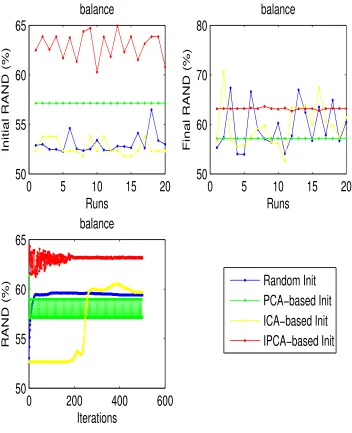
4.11 The clustering performance of random, PCA-based, ICA-based and
IPCA-based initialization for balance dataset . . . 58
4.12 The clustering performance of random, PCA-based, ICA-based and
IPCA-based initialization for cancer-int dataset . . . 59
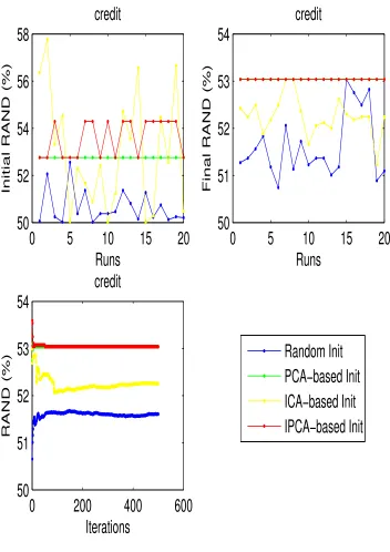
4.13 The clustering performance of random, PCA-based, ICA-based and
IPCA-based initialization for credit dataset . . . 60
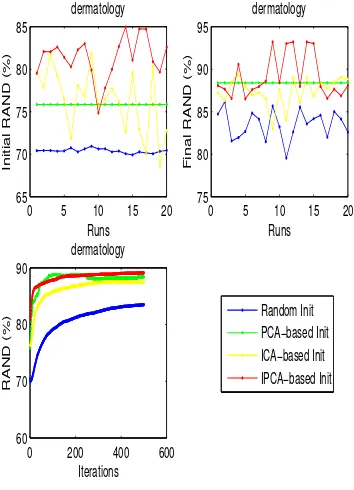
4.14 The clustering performance of random, PCA-based, ICA-based and
IPCA-based initialization for dermatology dataset . . . 61
4.15 The clustering performance of random, PCA-based, ICA-based and
IPCA-based initialization for diabetes dataset . . . 62
4.16 The clustering performance of random, PCA-based, ICA-based and
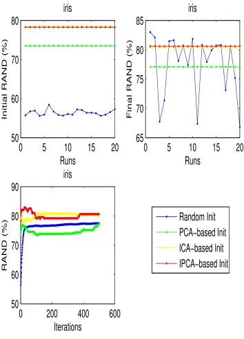
IPCA-based initialization for iris dataset . . . 63
4.17 The clustering performance of random, PCA-based, ICA-based and
IPCA-based initialization for thyroid dataset . . . 64
4.18 The clustering performance of random, PCA-based, ICA-based and
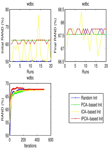
IPCA-based initialization for wdbc dataset . . . 65
4.19 The clustering performance of random, PCA-based, ICA-based and
IPCA-based initialization for wine dataset . . . 66
5.1 Data flow of the proposed ENMF. The circle, triangle and rectangle
symbols represent candidates derived during the generation of theS(tM),
S(tF) and S(tS) subsets, respectively. . . 71 5.2 The accuracies of the corresponding testing dataset for balance
(ENMF-MIX) . . . 79
5.3 The accuracies of the corresponding testing dataset for breasttissue
(ENMF-MIX) . . . 80
5.4 The accuracies of the corresponding testing dataset for cancer
(ENMF-MIX) . . . 81
5.5 The accuracies of the corresponding testing dataset for cancerint
(ENMF-MIX) . . . 82
5.6 The accuracies of the corresponding testing dataset for dermatology
(ENMF-MIX) . . . 83
5.7 The accuracies of the corresponding testing dataset for glass (ENMF-MIX) 84
5.8 The accuracies of the corresponding testing dataset for haberman
(ENMF-MIX) . . . 85
5.9 The accuracies of the corresponding testing dataset for iris (ENMF-MIX) 86
5.10 The accuracies of the corresponding testing dataset for thyroid
6.1 The general process of the proposed evolutionary optimization strategy 92
6.2 The flow chart of the proposed evolutionary optimization strategy . . . 93
6.3 The structure of the experimental process . . . 98
6.4 The summary results for Yale face dataset under the different data
com-pression methods with the sparsity measure . . . 100
6.5 The summary results for Yale face dataset under the different data
com-pression methods with the orthogonality measure . . . 101
6.6 The summary results for Yale face dataset under the different data
com-pression methods with both the sparsity and orthogonality measures . . 102
6.7 The basis images obtained from different methods for Yale with the
sparsity measure. (1) 1st row represents the basis images obtained from
random initialized NMF at the increasing iterations (iter=1, 50, 100, 200,
500) (2) 2nd row represents the basis images obtained from random acol
initialized NMF at the increasing iterations (iter=1, 50, 100, 200, 500)
(3) 3rd row represents the basis images obtained from k-means based
initialized NMF at the increasing iterations (iter=1, 50, 100, 200, 500) (4)
4th row represents the basis images obtained from FCM-based initialized
NMF at the increasing iterations (iter=1, 50, 100, 200, 500) (5) 5th row
represents the basis images obtained from the proposed evolutionary
optimization strategy at the increasing iterations (iter=1, 50, 100, 200,
500) . . . 103
6.8 The basis images obtained from different methods for Yale with the
orthogonality measure which is similar with figure6.7. . . 104
6.9 The basis images obtained from different methods for Yale with both the
sparsity and orthogonality measures which is similar with figure6.7. . . 105
6.10 The summary results for ORL face dataset under the different data
com-pression methods with the sparsity measure . . . 107
6.11 The summary results for ORL face dataset under the different data
com-pression methods with the orthogonality measure . . . 108
6.12 The summary results for ORL face dataset under the different data
6.13 The basis images obtained from different methods for ORL with the
sparsity measure. (1) 1st row represents the basis images obtained from
random initialized NMF at the increasing iterations (iter=1, 100, 200,
500, 1000) (2) 2nd row represents the basis images obtained from random
acol initialized NMF at the increasing iterations (iter=1, 100, 200, 500,
1000) (3) 3rd row represents the basis images obtained from k-means
based initialized NMF at the increasing iterations (iter=1, 100, 200,
500, 1000) (4) 4th row represents the basis images obtained from
FCM-based initialized NMF at the increasing iterations (iter=1, 100, 200, 500,
1000) (5) 5th row represents the basis images obtained from the proposed
evolutionary optimization strategy at the increasing iterations (iter=1,
100, 200, 500, 1000) . . . 110
6.14 The basis images obtained from different methods for ORL with the
orthogonality measure which is similar with figure6.13. . . 111
6.15 The basis images obtained from different methods for ORL with both
the sparsity and orthogonality measures which is similar with figure6.13. 112
7.1 The independent component matrix . . . 119
7.2 Histogram of k-means clustering result withK= 64 from the
unnormal-ized data . . . 120
7.3 The largest cluster (No 33 cluster) in the k-means clustering result with
K = 64 from the unnormalized data . . . 121
7.4 One of single-member clusters, No 31 cluster, in the k-means clustering
result with K= 64 from the unnormalized data . . . 122
7.5 Histogram of k-means clustering result withK= 64 from the normalized
data . . . 123
7.6 The profiles of the members in No.40 cluster in normalized data . . . 124
7.7 The profiles of the members in No.40 cluster in unnormalized data . . . 125
7.8 The profiles of the members in No.18 cluster in normalized data . . . 126
7.9 The profiles of the members in No.18 cluster in unnormalized data . . . 127
7.10 The profiles of the members in No.19 cluster in normalized data . . . 128
7.11 The profiles of the members in No.19 cluster in unnormalized data . . . 129
7.12 The list of clustering results we have got . . . 130
7.13 The mean and standard deviation of the numbers of memberships . . . 130
7.14 Number of clusters which contains ICs from more than seven (>7) subjects131
7.15 The clusters containing more than seven subjects in the ensemble
clus-tering results: K= 64 . . . 132
7.16 The clusters containing more than seven subjects in the ensemble
List of Tables
2.1 Kaufman Approach (KA) initialization method . . . 11
2.2 The procedure of FCM . . . 14
2.3 The procedure of kernel k-means and kernel FCM . . . 15
2.4 The procedure of SOON-2 . . . 17
3.1 The comparison between random and random acol intialization . . . 41
4.1 The parameters for the preprocessing . . . 45
4.2 The properties of the final datasets . . . 45
4.3 The range of the standard deviation for log2(D) . . . 46
4.4 The properties of the datasets . . . 55
4.5 The mean and standard deviation of inital RAND values of different intialization methods (iters=1, runs=20) . . . 56
4.6 The mean and standard deviation of final RAND values of different in-tialization methods (iters=500, runs=20) . . . 56
5.1 Details of the datasets used. . . 75
5.2 Performance comparison for different datasets in RAND, which is re-ported in percentage (%). The best performance is highlighted in bold, and the second best is underlined. . . 75
5.3 Performance improvement of ENFM over NMF under different initial-ization approaches. . . 76
6.1 The procedure for finding the best solutionWt∗ . . . 95
6.2 The summary results for Yale face dataset under the different data com-pression methods with the five measurements saying sparsity, orthog-onality, objective value, error and RAND index at the final iteration (iter=500) . . . 114
6.3 Statistical significance test (t-test) for the average ENMF and NMF after 5 runs shown in table 6.2 . . . 115
6.5 The summary results for ORL face dataset under the different data
com-pression methods with the five measurements saying sparsity,
orthog-onality, objective value, error and RAND index at the final iteration
Acknowledgement
I would like to express my deep gratitude to Dr. Tingting Mu, Prof.Nandi Asoke and
Dr. Al-Nuaimy Waleed, my research supervisors, for their patient guidance, enhusiastic
Nomenclature
KA Kaufman Approach
FCM fuzzy c-means
FSOM fuzzy self-organizing map
FART fuzzy adaptive resonance theory
FSVM fuzzy support vector machine
SVM support vector machines
SOM self-organizing map
SOON self-organizing oscillator networks
OPTOC one-prototype-take-one-cluster
SSMCL self-splitting-merging competitive learning
CSM cohesion-based self-merging
APV asymptotic property vector
PVI parametric validity index
MST mining spanning tree
NMF Nonnegative Matrix factorization
SVD singular value decomposition
HC hierarchical clustering
RI random initialization
RAI random acol initialization
RCI random c initialization
ICA independent component analysis
IPCA independent principal component analysis
Chapter 1
Introduction
1.1
Motivation and Objectives
Machine learning is a subfield of computer science and artificial intelligences that deals
with the design and development of systems. Over the last few decades, there have been
many significant advances in machine learning. More and more applications of machine
learning are found in many different fields like biomedical engineering and
communi-cations. Machine learning is very important not only because that the achievement
of learning in machines might help us understand how animal and humans learn, but
also the following engineering reasons [76]. We might be able to specify input/output
pairs but not a concise relationship between inputs and desired outputs. We would like
machines to be able to adjust their internal structure to produce correct outputs for a
large number of sample inputs and, thus, suitably constrain their input/output
func-tion to approximate the relafunc-tionship implicit in the examples. Also, machine learning
can be used to reach on-the-job improvement of existing machine designs, to capture
more knowledge than what humans would want to write down, to adapt to a
chang-ing environment to reduce the need for constant redesign, and to track as much new
knowledge as possible.
Clustering is one of the most useful tools for the large data analysis and is my first
re-search topic. It is known as unsupervised learning which is to group individual objects
or samples in a population within which the objects are more similar to each other
than those in other clusters. It has been used for decades in many fields, such as image
processing, data mining, artificial intelligence [113] and the microarray gene expression
data analysis in genomic research [48].
Compression is another useful tool for machine learning. It involves encoding
informa-tion using fewer bits than the original representainforma-tion [77]. Compression can be either
lossy or lossless. Lossless compression reduces bits by identifying and eliminating
sta-tistical redundancy. No information is lost in lossless compression. Lossy compression
reduces bits by identifying unnecessary information and removing it [46]. The process
also one of my research topics. Data compression is also widely used in backup utilities,
spreadsheet applications, and database management systems.
The objectives of this thesis are developing machine learning algorithms for clustering,
classification and compression, emphasis on nonnegative matrix factorization (NMF).
Nonnegative matrix factorization (NMF) has becoming an increasingly popular data
processing tool these years, widely used by various communities including computer
vision, text mining and bioinformatics. It is able to approximate each data sample in
a data collection by a linear combination of a set of nonnegative basis vectors weighted
by nonnegative weights. This often enables meaningful interpretation of the data,
mo-tivates useful insights and facilitates tasks such as data compression, clustering and
classification. These subsequently lead to various active roles of NMF in data
analy-sis, e.g., dimensionality reduction tool [11, 75], clustering tool[94, 82, 13, 39], feature
engine [40], source separation tool [38], etc. In this research work, the NMF algorithm
is explored, emphasis being laid on the topic of the initialization methods as well as
the optimization rule for NMF, to solve some data analysis problems. We propose two
initialization methods for NMF based on the clustering algorithm and dimensionality
reduction algorithm. We also propose two NMF updating strategies, which take
ad-vantage of the hybrid of different NMF initialization setups and evolves along different
directions to produce NMF approximations that suits better the accuracy purposes (i.e.
data clustering/classification and compression). Effectiveness of the proposed methods
is demonstrated thoroughly through benchmark testing and comparison with existing
approaches.
1.2
Original Contribution
A summary of the the main original contributions of this work are shown below on a
chapter-by-chapter basis.
Chapter 2
We review five clustering families representing five clustering concepts including fuzzy
clustering, kernel-based clustering, self-organizing clustering, self-splitting and merging
clustering and ensemble clustering.
Chapter 4
We propose two initialization methods for NMF based on the clustering algorithm and
dimensionality reduction algorithm. The modification of k-means clustering and
inde-pendent principal component analysis (IPCA) are chosen as the initialisation methods
Chapter 5
We propose the new evolutionary optimization strategy for NMF driven by three
pro-posed update schemes in the solution space, saying NMF rule, firefly rule and survival
of the fittest rule. This proposed update strategy facilitates the clustering problem by
using the system objective functions that make use of the clustering quality
measure-ments.
Chapter 6
We propose the new evolutionary optimization strategy for NMF by modifying the
proposed optimization strategy in chapter 5 to solve the image datasets compression
problem.
Chapter 7
we employ several standard algorithms to provide clustering on the application of
pre-processed EEG data. We also explore ensemble clustering to obtain some tight clusters.
1.3
Publications
Papers arisen from the this PhD work are listed as follows:
Journal Papers
1. Liyun Gong, Tingting Mu, Meng Wang, Hengchang Liu and John Y.
Gouler-mas, A robust nonnegative matrix factorization strategy with adaptive quality
control of data clusters, Pattern Recognition, 2014. (IF=2.632, under review)
2. FY Cong, V Alluri, AK Nandi, P Toiviainen, Rui Fa, Basel Abu-Jamous, Liyun
Gong, BGW Craenen, H Poikonen, M Huotilainen, T Ristaniemi, Linking Brain
Responses to Naturalistic Music through Analysis of Ongoing EEG and Stimulus
Features, IEEE Transactions on Multimedia, 15(5):1060-1069, 2013. (IF=1.776)
Conference Papers
1. Liyun Gong, T. Mu and Al-Nuaimy Waleed, Evolutionary nonnegative matrix
factorization for data compression, European Conference on Machine Learning
and Principles and Practice of Knowledge Discovery in Databases, 2015. (to be
submitted)
2. Liyun Gong and Asoke K. Nandi, Clustering by Non-negative Matrix
Factor-ization with Independent Principal Component InitialFactor-ization. European Signal
3. Liyun Gong and Asoke K. Nandi, An Enhanced Initialization Method for
Non-negative Matrix Factorization, IEEE International Workshop on Machine
Learn-ing for Signal ProcessLearn-ing, MLSP, 2013. (acceptance rate=51%)
4. Rui Fa, Asoke K Nandi and Liyun Gong, Clustering analysis for gene expression
data: a methodological review, 5th international symposium on communication,
Chapter 2
Clustering Analysis
This chapter describes the basis knowledge of clustering analysis and also reviews
some common clustering algorithms. Firstly section 2.1 provides a brief introduction
to machine learning, including supervised learning, unsupervised learning and
semi-supervised learning. Section 2.2 provides the comprehensive review of some popular
clustering algorithms in addition with the five clustering families representing five
clus-tering concepts. Since clusclus-tering is one of the most widely used unsupervised learning
technique, the task of assessing the results of clustering algorithms can be as important
as the clustering algorithms themselves. So several clustering validations are reviewed
including internal and external evaluations as well in section 2.3. The reason for this
chapter is that some methods described here have been selected to solve the brain
appli-cation in chapter 7 and also some of them were treated as the initialisation methods for
nonnegative matrix factorisation in chapter 5 and 6. Work of this chapter is published
in:
Rui Fa, Asoke K Nandi and Liyun Gong, Clustering analysis for gene expression data:
a methodological review, 5th international symposium on communication, control, and
signal processing, ISCCSP, 2012. (acceptance rate=48%)
2.1
Machine Learning
Machine learning is a subfield of computer science and artificial intelligences that deals
with the design and development of systems. It has been defined formally by Mitchel
[71] as ”A computer program is said to learn from experience E with respect to some
class of tasks T and performance measure M, if its performance at tasks in T, as
measured by M, improves with experience E.” Over the past 50 years, the study of
machine learning has grown from the efforts of a handful of computer engineers
explor-ing whether computers could learn to play games, and a field of statistics that largely
ignored computational considerations, to a broad discipline that has produced
funda-mental statistical-computational theories of learning processes; has designed learning
computer vision; and has spun off an industry in data mining to discover hidden
reg-ularities in the growing volume of online data [72]. A number of choices are involved
in designing a machine learning approach, including choosing the type of training
ex-perience, the target function to be learned, a representation for this target function,
and an algorithm for learning the target function from training samples [71]. Machine
learning is inherently a multidisciplinary field, which draws on results from artificial
intelligence, probability and statistics, optimization theory, computational complexity
theory, control theory, information theory, philosophy, and other fields.
Machine learning has been used in many applications including natural language
pro-cessing [22, 68, 74], handwriting recognition [60, 79, 80, 84], face and fingerprint
recogni-tion [47, 79, 80, 116], bioinformatics and cheminformatics [8, 42, 110], object recognirecogni-tion
in computer vision [102], image compression [114].
Types of Algorithms
Machine learning algorithms are organised into several forms including supervised
learn-ing, unsupervised learning and semi-supervised learning.
Supervised learning is the machine learning task of inferring a function from labeled
training data. The training data consist of a set of training examples. Each sample
consists of a pair of an input object (typically feature vector) and a desired output
(tar-get). The output of the function can be used for calculating new examples (regression),
or can determine the class labels for unseen input objects (classification). In order to
solve a given problem of supervised learning, one has to consider six issues.
1. Determine the type of training samples.
2. Gathering a training set that contains information of problem. Thus, a set of
input objects and the corresponding outputs are gathered, either from human
experts or from measurements.
3. Determine the input feature representation of the learned function (feature
ex-traction). The accuracy of the learned function depends strongly on how the
input object is represented. Typically, the input object is transformed into a
feature vector, which contains a number of features that are descriptive of the
object. The number of features should not be too large, because of the curse of
dimensionality; but should be large enough to predict the output accurately.
4. Determine the structure of the learned function and corresponding learning
al-gorithm.
gathered training set. Parameters of the learning algorithm may be adjusted by
optimizing performance on a subset of the training set (called a validation set)
or via cross-validation. After parameter adjustment and learning, the
perfor-mance of the algorithm may be measured on a test set that is separate from the
training set.
6. Evaluate the accuracy of the learned function. After parameter adjustment and
learning, the performance of the resulting function should be measured on a test
set that is separate from the training set.
Unsupervised learning is the other form of machine learning which tries to find hidden
structure in unlabelled data. It is distinguished from supervised learning by the fact
that there is no a priori output. In unsupervised learning, a data set of input objects
is gathered, and treated as a set of random variables. A joint density model is then
built for the data set. Unsupervised learning can be used in conjunction with Bayesian
inference to produce conditional probabilities for any of the random variables given
the others. A holy grail of unsupervised learning is the creation of a factorial code of
the data, which may make the later supervised learning method work better when the
raw input data is first translated into a factorial code. Unsupervised learning is also
useful for data compression. Another form of unsupervised learning is clustering which
is introduced in details later.
Semi-supervised learning is a class of supervised learning tasks and techniques that also
make use of unlabeled data for training–typically a small amount of labeled data with
a large amount of unlabeled data. Semi-supervised learning falls between unsupervised
learning (without any labeled training data) and supervised learning (with completely
labeled training data). Many machine-learning researchers have found that unlabelled
data, when used in conjunction with a small amount of labeled data, can produce
considerable improvement in learning accuracy. The acquisition of labeled data for a
learning problem often requires a skilled human agent. The cost associated with the
labelling process thus may render a fully labeled training set infeasible, whereas
acqui-sition of unlabelled data is relatively inexpensive. In such situations, semi-supervised
learning can be of great practical value.
2.2
Clustering Algorithms
Clustering is one of the most useful tools for the large data analysis and is the one
of my research topics. It is known as unsupervised learning and has been used for
decades in many fields, such as image processing, data mining, artificial intelligence
[113] and the microarray gene expression data analysis in genomic research [48]. The
within which the objects are more similar to each other than those in other clusters.
Generally speaking, to study or design a clustering analysis for an application, one has
to consider three issues:
1. the measurements of the dissimilarity (or similarity)
2. the clustering algorithms
3. the clustering validations
There has been a rich literature on clustering analysis over the past decades and all these
three issues have been comprehensively discussed in [48] and [113]. However, as it has
been a few years since those two comprehensive review papers [48, 113] were published,
many new and effective algorithms have been proposed but were not reviewed. Both
the clustering algorithms and validations have grown beyond the horizon of [48, 113].
The following sections can be viewed as a complementary counterpart to make the
literature review in this field some-how up-to-data.
In section 2.2.2, we review some popular clustering algorithms, saying means,
k-medoids and hierarchical clustering. Besides some popular clustering algorithms, we
will also discuss five different families of clustering algorithms including fuzzy clustering,
kernel-based clustering, self-organizing clustering, self-splitting and merging clustering
and ensemble clustering in section 2.2.3-2.2.7.
2.2.1 Problem setting
There were seven similarity and dissimilarity measures listed in [113], namely,Minkowski
distance, Euclidean distance, City-block distance, Mahalanobis distance, Pearson
cor-relation, Point symmetry distance, Cosine similarity, which have been widely used in
various applications. In [48],Euclidean distance and Pearson correlation were claimed
to be effective similarity measures for gene expression data. Pearson correlation
mea-sures the similarity between two genes, and provides a very informative visualisation of
the clustering results. Based on a sample of paired genes (X, Y), the pearson correlation
is:
P C = 1
n−1 n
X
i=1
(Xi−X¯ SX
)(Yi−Y¯ SY
) (2.1)
where
¯
X= 1
n n
X
i=1
Xi; (2.2)
SX =
v u u t
1 n−1
n
X
i=1
(Xi−X¯)2 (2.3)
are the mean and the standard deviation forX and nis the number of dimensions for
X. (The terms forY are similar.)
metrics on Euclidean space which can be considered as the generalization of the
Eu-clidean distance. TheMinkowski distanceof orderpbetween two pointsX = (x1, x2, ..., xn) and Y = (y1, y2, ..., yn) is defined as:
M inD= ( n
X
i=1
|xi−yi|p)
1
p (2.4)
Minkowski distance is typically used with p being 1 or 2. The latter is the Euclidean
distance, while the former is known as City-block distance.
Mahalanobis distance is equated to the euclidean distance in a transformed whitened
space. Given an sample x = (x1, x2, x3, ..., xN)T from a group of samples with mean µ= (µ1, µ2, µ3, ..., µN), this distance is defines as:
M ahD(x) =
q
(x−µ)TS−1(x−µ) (2.5)
whereS is the covariance matrix of this group of samples. IfS is the identity matrix,
Mahalanobis distance reduces toeuclidean distance.
Point symmetry distanceis the distance which incorporates both the Euclidean distance
as well as a measure of symmetry. Given N samples xi, i = 1, ..., N and a reference
samplec, the distance between a sample xj and the reference sample cis defined as:
P D(xj, c) =minj=1,...,N;i6=j
||(xj−c) + (xi−c)||
||xj −c||+||xi−c||
(2.6)
where the denominator term is used to normalize the point symmetry distance so as to
make the point symmetry distance insensible to the Euclidean distances||xj −c|| and
||xi−c||.
Cosine similarity is a measure of similarity between two vectors of an inner product
space that measures the cosine of the angle between them. Given two samples/vectors
X and Y, the cosine similarity,cos(θ), is calculated using the dot product and
magni-tudes ofX and Y as
CosS=cos(θ) = X·Y
||X||||Y|| (2.7)
The resulting similarity ranges from -1 meaning exactly opposite, to 1 meaning exactly
the same, with 0 usually indicating independence, and in-between values indicating
intermediate similarity or dissimilarity.
Furthermore, two additional measures, namely Jackknife correlation and Spearman’s
rank-order correlation, were discussed to cope with the situations of outliers and
non-Gaussian distributions, respectively. In the following sections of this chapter, we will
not discuss the dissimilarity and similarity measures but use the operatorsD(·) for dis-similarity andS(·) for similarity instead of a specific measure when we study clustering algorithms. Readers who are interested in more details are advised to refer to [113, 48]
Here we suppose that we are going to partition the dataset X = {xn|1 ≤ n ≤ N}, where xn ∈ RM×1 denotes the n-th object, M is the number of samples (features or
dimensions) and N is the number of objects. Consider that there are K clusters in a
given dataset and each clustering algorithm provides a partition matrix UK×N, where the entry uk,n ∈ [0,1] represents the membership coefficient of n-th object in the k-th cluster.
2.2.2 Popular Clustering Algorithms
K-means Clustering
The k-means clustering algorithm is one of the simplest and most common partitioning
methods.[64, 66]. For the traditional k-means, it starts with thekcluster centers chosen
randomly, where k is the cluster number. Using distance methods such as Euclidean
distance to measure the similarity between data objects and the cluster centers. Thus,
it leads to the following objective function:
E=
K
X
j=1
X
xi∈Cj
||xi−uj||2 (2.8)
whereCj denotes thej-th cluster, ujis the center of the clusterj which is the mean of
objects inCj andxi is the observations to be clustered. Each object is then assigned to
one of the cluster groups with the closest center. Then the cluster centers are redefined
by finding the mean vector of all objects belonging to each cluster group and the objects
are reassigned according to their distance to these new cluster centers. This iterative
process repeats until there are no changes in the assignment of objects to cluster groups.
The algorithm is often presented as assigning objects to the nearest cluster by distance.
The standard algorithm aims at minimizing the Euclidean objective, and thus assigns
by ”least sum of squares”. Using a different distance function other than the squared
Euclidean distance may stop the algorithm from converging. Various modifications of
k-means such as spherical k-means [89] and k-medoids [52] have been proposed to allow
using other distance measures. For example, k-medoids chooses objects as centers and
works with an arbitrary matrix of distances between objects instead ofL2. This method
was proposed in [52] for the work withL1 norm and other distances.
Since different starting points can result in the different cluster results, it may be
advisable to run the algorithm several times and select the best solution among them.
Also in literature, some initialization algorithms have been proposed to the traditional
k-means clustering to avoid the influence of the randomness [83]. Here we review
the Kaufman Approach (KA) proposed by Kaufman and Rousseeuw [53] which is the
Table 2.1: Kaufman Approach (KA) initialization method
STEP1: Select the first center so that it has the minimum distance to the other objects.
STEP2: For every nonselected objectwj: CalculateCji =max(Dj−dji,0),
where dji is the absolute distance between wi and wj. wi is the second randomly selected center.
Dj is the minimum distance between the pre-selected centers andwj. STEP3: Calculate P
jCji for the currentwi.
STEP4: Repeat STEP2 and STEP3 and select the second centerwiwhich maximizes
P
jCji.
STEP5: Iterative process continues untilk initial centers are selected.
The main disadvantage of the k-means clustering algorithm is the predefined cluster
number. It is difficult to set the number of cluster since most of the real datasets are
unknown.
K-medoids
The k-medoids is one of many partitioning algorithms, which is an extension of the
k-means. The k-medoids is designed to handle the outliers efficiently. Instead of using
the means, it chooses the medoids to represent the cluster centers. A medoid is the
most centrally located object within a cluster, whose total distance to all other objects
intra-cluster is the shortest. Similar to the k-means, the k-medoids keeps updating the
medoids if cluster membership changes until the process converges.
Hierarchical Clustering (HC)
In contrast to partition-based clustering, which directly divides the data set into
dis-connected parts, HC is path-based clustering algorithm, which generates a hierarchical
series of nested and connected clusters. This nested cluster structure can be graphically
represented in a tree bydendrogram. There are two approaches to implement the HC:
one is called agglomerative which initially regards each data object as an individual
cluster and merges the closest pair of clusters at each step, until all the groups are
merged into one cluster; The other is called divisive, which starts with one cluster
con-taining all the data objects and splits singleton clusters at each step. In this thesis,
we employ agglomerative clustering. HC provides different clustering results when
em-ploying different linkage criteria. The linkage criteria determine the distance between
clusters as a function of the pairwise distances between objects.
Single Linkageuses the distance between the nearest neighbours. For example, if we
have two clustersAand B, the single linkage distance is defined as
d(A, B) = min
α=1,...,nAβ=1,...,nB
d(aα, aβ) (2.9)
between two points.
Figure 2.1: The single linkage (nearest neighbour) distance), from [30]
Complete linkage uses the maximum distance between objects.
d(A, B) = max
α=1,...,nAβ=1,...,nB
d(aα, aβ) (2.10)
Figure 2.2: The complete linkage distance, from [30]
Average linkage uses average distance of objects.
d(A, B) = 1 nAnB
nA X
α=1
nB X
β=1
Figure 2.3: The average linkage distance, from [30]
Ward Linkage: In ward linkage, the distance between two clusters is the ANOVA
sum of squares between the two clusters added up over all the objects.
There are other linkage such as centroid linkage which uses the variance of the merging
clusters.
2.2.3 Fuzzy clustering
Fuzzy clustering is a concept that relaxes the restriction of crisp clustering, which
assigns every object exactly in one clusters, by characterizing the membership of each
sample point in all the clusters with a membership function which ranges between zero
and one. Additionally, the sum of the memberships for each sample point must be
unity [9]. The properties of the partition matrix is mathematically expressed by
1. uk,n ∈[0,1], 1≤n≤N,1≤k≤K 2. PK
k=1uk,n = 1, 1≤n≤N 3. 0<PN
n=1uk,n<N, 1≤k≤K
An example of fuzzy clustering is the fuzzy c-means (FCM) [10], which is fuzzy
counterpart of the k-means. FCM aims to minimize the cost function, which is
math-ematically expressed by
φ(U,X) = K
X
k=1
N
X
n=1
(uk,n)mD(xn,ck) (2.12)
where m∈[1,∞) is the fuzzification parameter. D(xn,ck) is the dissimilarity mea-sure between thenthobject,xn, and the center of thekthcluster,ck. Similar to k-means,
the cost function 2.12 can be minimised with an iterative procedure that updates the
partition matrix and the centers of clusters alternately. Since many objects may
par-ticipate in more than one function in the process, the fuzzy clustering has obvious
advantage to identify some objects co-regulating with more than one cluster of objects.
The procedure of FCM is summarized in Table 2.2. There are also many other fuzzy
clustering approaches, for example, fuzzy self-organizing map (FSOM) [81], fuzzy
Table 2.2: The procedure of FCM
STEP1: Initialize the centers of clusters {ck|k = 1, ...,K} randomly or based on some prior knowledge if available;
STEP2: Update the membership matrixU byuk,n = 1/
h PK
k0=1(
D(xn,ck0)
D(xn,ck))
2/(1−m)i,
k= 1, ..., K and n= 1, ..., N.
STEP3: Update the centroids of clusters{ck|k= 1, ...,K} byck(t) =
PN
n=1umk,nxn PN
n=1umk,n
for
k= 1, ..., K.
STEP4: Repeat STEP2 and 3 until ||C(t)−C(t−1)|| < , where is a small positive number.
2.2.4 Kernel-based clustering
Kernel-based clustering, which shares similar idea with support vector machines (SVM),
constructs a hyperplane to separate the patterns. These patterns are nonlinearly
trans-formed from a set of nonlinearly separable patterns into a higher-dimensional feature
space to be linear separable. At the core of the kernel-based clustering lies the difficulty
of explicitly constructing the nonlinear mapping, Φ(·), which is sometime infeasible; but now it can be overcome by a kernel trick. The kernel trick is a way of mapping
pat-terns from a input space into a feature space without having to compute the mapping
explicitly, in the hope that the patterns will gain meaningful linear structure in the
feature space, mathematically expressed as
k(xi, xj) = Φ(xi)TΦ(xj) (2.13)
where (·)T is the transpose operator. Thus, a straightforward way to transform the calculation of Euclidean distance in the feature space into the kernel version is to use
the kernel trick as follows.
DEk(Φ(xi),Φ(xj)) =||Φ(xi)−Φ(xj)||2
=||Φ(xi)||2+||Φ(xj)||2−2Φ(xi)TΦ(xj)
=k(xi, xi) +k(xj, xj)−2k(xi, xj) (2.14)
Correlation between sets of data is a measure of how well they are related. The
most common measure of correlation in stats is the Pearson Correlation. It shows the
linear relationship between two sets of data. The kernel version of modified Pearson
correlation is given by [86].
SPk(Φ(xi),Φ(xj)) =
Φ(xi)TΦ(xj)
p
Φ(xi)TΦ(xi)p
Φ(xj)TΦ(xj)
= p k(xi, xj)
k(xi, xi)
p
k(xj, xj)
Kernel k-means (or kernel FCM) is kernel counterpart of the k-means (or FCM)
[26], whose core part is to calculate the distance between the objects and the centroids
of clusters in the feature space.
DEk(Φ(xi), cΦk) =||Φ(xi)− 1 Nk
N
X
l=1
umk,lΦ(xl)||2=k(xi, xi)− 1 Nk
N
X
l=1
umk,lk(xi, xl)
+ 1 Nk2
N X l=1 N X n=1
umk,lumk,nk(xl, xn) (2.16)
where Nk =
PN
l=1umk,l. For crisp kernel k-means, the elements in partition matrix are either zero or one and m = 1; for the kernel FCM, the partition matrix is the
one described in Section 2.2.3 and m ∈ [1,∞). The procedure of kernel k-means and kernel FCM is summarised in Table 2.3. Other kernel-based algorithms including kernel
hierarchical and kernel principle component analysis can be found in [86, 63]
Table 2.3: The procedure of kernel k-means and kernel FCM
STEP1: Initialize a K-partition in the feature space;
STEP2: CalculateDkE Φ(xn), cΦk
forn= 1, ..., N and k= 1, ..., K.
STEP3: Update the membership matrix U(t) by
uk,n=
1 DkE Φ(xn), cΦk< DkE Φ(xn), cΦk0
0 otherwise (2.17)
for kernel k-means;
uk,n = 1/
PK
k0=1(
Dk
E(Φ(xn),cΦk0)
Dk
E(Φ(xn),cΦk)
)2/(1−m)
, for kernel FCM.
STEP4: Repeat STEP2 and 3until PK
k=1DEk cΦk(t), cΦk(t−1)
< , whereis a small positive number.
2.2.5 Self Organizing Clustering
The Kohonen self-organising map (SOM) is one of the most popular unsupervised
clus-tering algorithms [51, 100] and has been reviewed in many references [113, 48]. There
is another algorithm, called self-organizing oscillator networks (SOON) [91], which also
belongs to self-organizing clustering family. The so-called self-organizing means that
all the prototypes are attracted to the input patterns in an adaptive fashion. Here, we
focus on the SOON algorithm, which makes use of a biological fact that fireflies flash
together exhibiting a synchronised firing in groups that physically close to each other.
The basic unit of clustering in SOON is an integrate and fire (IF) oscillator representing
each object in the dataset.
Suppose that O = {O1, ...,ON} is a set of N oscillators, where each oscillator Oi is characterised by a phase φi and a state variable si, given by
where each functionfi : [0,1]→[0,1] is smooth. In [91], the functionf(φ) was
f(φ) = 1 bIn
h
1 + (eb−1)φ
i
. (2.19)
whenever si reaches a threshold atsi = 1, thei-th oscillator fires and instantaneously
reset to zero, following which the cycle repeats. The firing of all other oscillators
Oj(j6=i) can be affected byi-th oscillator by
sj(t+) =B(sj(t) +i(φj)), (2.20)
whereB(·) is a limiting function to guarantee thatsj(t) is confined to [0,1], math-ematically expressed by
B(s) =
s if 0≤s≤1 0 if s <0 1 if s >1
(2.21)
The coupling strength of thei-th oscillator at a given phaseφj,i(φj), is the most
important concept of the SOON algorithm, mathematically expressed by
i(φj) =
CE h
1−(D(Oi,Oj)
δ0 )
2i if D(O
i,Oj)≤δ0
−CI
h
(D(Oi,Oj)−δ0
δ1−δ0 )
2i if δ
0< D(Oi,Oj)≤δ1
−CI otherwise
(2.22)
whereδ0 andδ1 are limit distances andδ1 is set to be five timesδ0. CE andCI are the maximum excitatory coupling and the maximum inhibitory coupling, respectively.
To avoid the need to compute and store the pairwise distances between any pair of
Table 2.4: The procedure of SOON-2
STEP1:
Initialize a phasesφi randomly for i= 1, ..., N;
SetK , and initialize the Prototypes βk randomly fork= 1, ..., K;
STEP2:
Identify the next oscillator to fire, {Oi:φi =maxjφj}; Identify the close prototype to the oscillatorOi 7→βk; Compute D(βk,Oi) for ∀j ∈[1, N];
Bringφi to threshold, and adjust other phases φj =φj+ (1−φi) for ∀j∈[1, N];
STEP3:
forall oscillatorsOj(j 6=i)do
Compute state variable sj ; Compute coupling strengthi(φj); Adjust state variablesj using (2.20);
Compute compute new phase usingφj =f−1(sj);
end for
Identify synchronized oscillators and reset their phases; Update prototypeβk;
STEP4:
RepeatSTEP 2 and 3 until synchronized group stabilize.
2.2.6 Self Splitting and Merging Clustering
Self-splitting and merging clustering is an idea in which without setting the number of
clusters a priori, the algorithm will converge to a partitioning which reveals the true
number of clusters and provides fairly accurate clustering results. Recently, some self
splitting-merging clustering algorithms have been developed for both general purpose
clustering [120, 59] and gene expression data analysis [111]. A competitive learning
paradigm, called one-prototype-take-one-cluster (OPTOC) [120], was proposed in the
self-splitting clustering algorithm. There are two advantages of the OPTOC that,
firstly, it is not sensitive to initialization, and secondly, in many cases, it is able to find
natural clusters. However, its ability to find the natural clusters depends on the
deter-mination of suitable threshold, which is difficult [111]. Being aware of the
shortcom-ing of the OPTOC, a self-splittshortcom-ing-mergshortcom-ing competitive learnshortcom-ing (SSMCL) algorithm
[111] based on the OPTOC paradigm was developed for gene expression analysis. The
SSMCL initially over-clusters the whole dataset using the OPTOC principle and then
merge the groups based on the second order statistical characteristics. However,
al-though the number of clusters can be initially set to any value lager than the number
of natural clusters, the SSMCL still needs to set it as close to the number of natural
clusters as possible, otherwise, too much computing power will be wasted due to the
unnecessary over-clustering and merging. With the similar principle as the SSMCL,
over-clustering and merging, a cohesion-based self-merging (CSM) algorithm, which
same problem of setting the initial number of clusters. Here, we briefly introduce the
OPTOC competitive learning paradigm. For each prototype, an online learning vecoter
called asymptotic property vector (APV),Ak, is assigned to guide the learning thek-th
prototypePk. The APV is adapted according to
Ak=Ak+ 1
nkA ·δk·(xn−Ak)Θ(Pk, Ak, xn) (2.23) where
nkA=nkA+δk·Θ(Pk, Ak, xn),Θ(a, b, c) =
1 if D(a, b)≤D(a, c)
0 otherwise (2.24)
and
δ=
D(Pk, Ak) D(Pk, xn) +D(Pk, Ak)
(2.25)
The learning process for Pk is given by
Pk=Pk+αk·(xn−Pk)Θ(Pk, Ak, xn) (2.26)
where
αk =
1 + D(Pk, xn) D(Pk, Ak)
−2
(2.27)
The above OPTOC competitive learning paradigm is an effective technique to
im-plement the self splitting and merging clustering.
2.2.7 Ensemble Consensus Clustering
Robustness is one of the desired properties of clustering algorithms, However, there
is no perfect method which always gives the best results for all types of datasets. In
order to enhance the robustness of clustering, the idea of ensemble consensus clustering
has been proposed where the partitioning results of many clustering experiments are
combined [97, 73, 34, 98, 5, 103, 106, 6]. These partitioning results may come from
different clustering algorithms, or same clustering algorithm with different parameters
and initializations, or same clustering algorithm to different re-sampled permutations
of the target dataset. Although cluster ensembles have been regarded as promising
methods, many obstacles have been found while combining results from different
ex-periments. Due to the fact that clustering is unsupervised, one main problem is that
it is not a straightforward task to map a specific cluster from one of the clustering
results to its corresponding cluster from another clustering result. Another problem is
that different clustering results may give different numbers of clusters while the correct
number of clusters in unknown. Consensus function method has been employed as an
essential step in cluster ensembles. ForRpartitions{U1, ..., UR}, the optimal consensus partitionU∗ is the one which is the most similar to all of them and is mathematically given by
U∗ =argmax∀P
R
X
j=1
where Γ(·,·) measures the similarity between any two partitions. This optimization problem has been noted as an NP-complete problem. There are many methods for
consensus function, including relabelling and voting [6], co-association matrix [37],
hyper- graph methods [97], weighted kernel consensus functions [103], non-negative
matrix factorization [106], greedy algorithms [34], etc. In all of the aforementioned
methods, there are at least three steps to implement the ensemble consensus clustering
as follows:
• Partitions generation: R different clustering experiments are carried out to generate R partitions. The results of these partitions are all presented in a
con-sistent form known as the partition matrix.
• Relabelling: The clusters in the generated partitions are relabelled such that the corresponding clusters from different partitions are aligned.
• Final consensus partition matrix generation: The relabelled partition ma-trices are ”assembled” to generate the final consensus partition matrix.
Among these three steps, Relabelling and Final consensus partition matrix
gener-ation are the most essential parts. An example of relabelling is detailed in the steps
below:
1. A dissimilarity distance matrixSK×K is constructed by calculating the pairwise distance between the rows (clusters) of the matrixU and the rows of the
refer-ence matrixUref.
2. The minimum value in each of the columns is found.
3. The maximum value of these minima is identified then the rows (clusters) from
U and Uref which correspond to this similarity value are mapped.
4. The row and the column which show the aforementioned value are deleted from
the similarity matrix.
5. If all of the K rows from U and Uref are mapped, the algorithm terminates,
otherwise it goes back to step (2) with the reduced similarity matrix.
It is suggested that an intermediate consensus partition matrixUint(k)is initialized with the values of the first partition U1, and then the other partitions are relabelled and fused with this intermediate matrix one by one while considering it as the reference
at each step. Mathematically, let ˆUr be the relabelled partition matrix of the partition
relabelling and fusing the partitions {U1, ...,Uk}. Let the function Relabel(U, Uref ) denote relabelling the partition matrixU by consideringUref as the reference partition.
Equation 2.14 shows how the intermediate partition matrix can be calculated by the
normal approach and the recursive approach:
Uint(k)= 1 k
k
X
r=1
ˆ Ur = 1
k ˆ
Uk+(k−1)
k U
int(k−1) (2.29)
An example of generating the final consensus partition matrix is achieved by
fol-lowing the algorithm shown in the folfol-lowing steps:
1. Uint(1) =U1
2. For k= 2 to R
a.Uˆk=Relabel(Uk,Uint(k−1)) b.Uint(k)= 1kUˆk+(k−k1)Uint(k−1)
3. U∗=Uint(R)
2.3
Clustering validation
Since clustering is unsupervised classification, it is more difficult to assess than a
su-pervised approach. Thus, the task of assessing the results of clustering algorithms can
be as important as the clustering algorithms themselves. There are two functional
advantages of employing the clustering validations: firstly, they can validate a
clus-tering algorithm by comparing with other algorithms; secondly, some validity indices
can provide an estimate of the number of clusters, which is crucial information for the
clustering analysis. In this section, we will review two types of the existing clustering
validations including internal evaluating and external evaluating. When internal
eval-uation is used, the assessment is based on the data matrix itself. The cluster structure
possessing higher within-cluster similarity and lower between-cluster similarity is of
better quality. When external evaluation is used, the assessment compares the
cluster-ing results with the ground truth partition of the dataset. The cluster structure that
better matches the ground truth partition is of higher quality.
2.3.1 Internal Evaluation
Bayesian information criterion index (BIC)
The Bayesian information criterion (BIC) has been proposed in [3] and is defined as:
Where n is the number of objects, L is the likelihood of the parameters to generate
the data in the model, and v is the number of free parameters in the Gaussian model.
Smaller BIC value means better clustering performance.
Davies-Bouldin index (DB)
This index DB [21] is defined as:
BD= 1
c c
X
i=1
M axi≤j
d(Xi) +d(Xj) d(ci, cj)
(2.31)
Werec denotes the number of clusters,i,j are cluster labels, thend(Xi) andd(Xj) are
all samples in clusters iand j to their respective cluster centroids, d(ci, cj) is the
dis-tance between these centroid. Smaller DB value means better clustering performance.
Parametric Validity Index
A parametric validity index (PVI), which employs two tunable parameters α andβ to
to control the proportions of objects that are involved in the calculation of the
intra-cluster dissimilarities and the inter-intra-cluster dissimilarities, was proposed in [33]. For
each cluster, three spaces are defined, namely the inner space, the intra outer space
and the inter outer space, representing the objects inside the cluster chosen for the
calculation of both the intra-cluster dissimilarities and the inter-cluster dissimilarities,
the objects inside the cluster chosen for the calculation of only the intra-cluster
dis-similarities, and the objects outside the cluster chosen for the calculation of only the
inter-cluster dissimilarities, respectively. Let Ni k , Nao
k , Neok denote the numbers of
objects in the inner space, the intra outer space and the inter outer space, respectively,
for thekith cluster. The fractions, α and β, are used to control Nki ,Nao
k ,Neok, which
can be expressed as
Nki =dαNke;Nao
k =dβNke;Neok =dβ(N −Nk)e; (2.32)
where Nk is the number of the objects in the kith cluster, N is the number of all
objects in the dataset and d·e is the ceiling operator. Both α and β can be chosen from the range of (0,1]. Thus, the inner space is Ak = {aka|a = 1, ..., Nki}, the intra outer space is Bka = {ba,bk |b = 1, ..., Nao
k}, and the inner outer space is C
a k ={c
a,c k |c = 1, ..., Neo
k}. The PVI is obtained by
P V I(K, α, β) = K X k=1 Ni k X a=1
(De
a k
Daa k
) (2.33)
where
Daa k =
PNaok
b=1 D(aak, b a,b k )
Nao ;De
a k =
PNeok
c=1D(aak, c a,c k )
Other Indices
Here we also list five other existing validity indices. The first is theVI [92]. The validity
indexVIis the ratio of the inter-cluster separation measures and the intra-cluster scatter
measures, which is mathematically expressed as
VI(K) =
PK
i=1Iei PK
i=1Iai
(2.35)
where K is the number of clusters. The VI employs Iai, the largest dissimilarity of
the minimum spanning tree (MST) for cluster i, as the intra-cluster scatter and Iei =
minKj=1,j6=iIeij , where Ieij is the the largest dissimilarity of the MST for cluster i and
cluster j, as the inter-cluster separation.
The second is theDI[29], which is written as
DI(K) =min1≤i≤K[min1≤i≤K[
δ(Ci, Cj) max1≤k≤K[∆(Ck)]
]] (2.36)
where δ(Ci, Cj) =min||xi−xj||2 is the maximum distance between cluster i and
cluster j, ∆(Ck) is the largest intra-cluster separation of cluster k. The third is the II
[70], which is written as
II(K) = (1
K ×
E1
EK
×DK)P (2.37)
where E1 = Pj||xj −c||2 where c is the centroid of the whole dataset, EK =
PK
k=1
P
j∈Ck||xj −ck||2, DK =max
K
i,j||ci −cj||2 and power P is constant, which is 2
in our experiments. The fourth is theGI [54], which is expressed as
GI(K) =max1≤k≤K[
(2PM
m=1
√
λmk)2 min1≤j≤K||ui−uj||2
] (2.38)
where M is the number of dimensions, λmk are the eigenvalues of the covariance
matrix of the k-th cluster. Note that the closest GI value to zero suggests the best
number of clusters. The fifth is theCH [16] which is given by
CH(K) = [
PK
k=1nk||ck−u||2
K−1 ]
[
PK k=1
Pnk
i=1||xi−ck||2
n−K ]
(2.39)
wherenk is the number of memberships in the cluster k and n is the total number of
the objects.
2.3.2 External Evaluation
RAND
RAND [87] is defined as the probability of correction for the cluster results. It handles
cluster labels and Q records the cluster labels obtained from the algorithms. So the
RAND indexw∈[0,1] is then defined as
w= a+d
a +b+c+d ×100% (2.40)
where a represents the number of pairs of data points belonging to the same cluster
both inT and in Q,b represents the number of pairs of data points belonging to the
same cluster in Tbut different clusters inQ,c represents the number of pairs of data
points belonging to different clusters inTbut the same cluster in Q, andd represents
the number of pairs of data points belonging to different clusters both inT and inQ.
Note that a RAND value closer to one suggests the better cluster result.
Normalized Mutual Information (NMI)
The NMI of two labeled objects can be measured as:
N M I(X, Y) = p I(X, Y)
H(X)H(Y) (2.41)
Where,I(X, Y) denotes the mutual information between two random variablesX and
Y andH(X)denotes the entropy ofX. X is clustering result while Y will be the true
labels.
Purity
The purity of the clustering solution is obtained as:
P urity= m
X
j=1
nj
nPj (2.42)
were nj is the size of clusterj,m is the number of clusters andn is the total number
of objects. Pj is the purity in cluster j and computed as follows.
Pj = 1 nj
M axi(nij) (2.43)
The equation is the number of objects inj with class labeli.
Entropy
Entropy measures the purity of the clusters class labels. Thus, if all clusters consist of
objects with only a single class label, the entropy is 0. However, as the class labels of
objects in a cluster become more varied, the entropy increases. To compute the entropy
of a dataset, we need to calculate the class distribution of the objects in each cluster
as follows:
Ej =
X
i
Where the sum is taken over all classes. The total entropy for a set of clusters is
calculated as the weighted sum of the entropies of all clusters, as shown in the next
equation.
E =
m
X
j=1
nj
nEj (2.45)
Werenj is the size of clusterj,mis the number of clusters, and nis the total number
of data points.
2.4
Summary
In this chapter, we reviewed some popular clustering algorithms including k-means,
k-medoids and HC. Also five families of cpustering algorithms are summarised and
discussed in one of our conference papers. All these clustering methods here can be
used as the clustering based initialisation for NMF. In chapter 4, 5 and 6, we selected
k-means and FCM as the examples for NMF initialisation and chose RAND as the
measure of the clustering performance. Future works can be done using other clustering
methods and clustering validations. In chapter 7, k-means, k-medoids and HC were used
to analyse the clustering performance of EEG dataset. Also the ensemble clustering
Chapter 3
Nonnegative Matrix
Factorization
This chapter describes the knowledge of Nonnegative matrix factorisation (NMF),
em-phasis on the topic of both NMF optimization strategies and NMF initialization
meth-ods. Section 3.1 provides a brief concept of NMF and its usages. Section 3.2 reviews
some NMF optimization strategies. Section 3.3 introduces three types of NMF
initial-ization methods saying randomisation-based initialisation, cluster-based initialinitial-ization
and dimensionality reduction-based initialiszation.
3.1
Introduction
NMF, proposed by [24], is an algorithm based on decomposition by parts that can
reduce the dimensionality of the datasets while keeping the most information about
the datasets. It is different from principal component analysis (PCA) and independent
component analysis (ICA) with the added non-negative constraints. Researchers have
proposed several different algorithms based on the traditional NMF to make
improve-ments such as Least squares-NMF [105], Weighted-NMF [41], Local-NMF [56], and so
on. Here we briefly review the idea of NMF as follows. Given a nonnegative matrix
X= [xij] with m rows and n columns, the NMF algorithm seeks to find nonnegative
factorsW= [wij] andH= [hij] such that
X ≈ WH (3.1)
whereWis anm×kmatrix andHis ak×nmatrix. Each column of W is considered as the basic vectors while each column of H contains the encoding coefficient. k here
is the rank of dimensionality and normally smaller than m and n for the aim of the
dimensionality reduction. All the elements inWand Hrepresent non-negative values.
NMF method has been found to be useful tool in both data compression and data
![Figure 3.5: Prostate cancer study: sample representation using the first two or threecomponents from PCA, ICA and IPCA, from [118]](https://thumb-us.123doks.com/thumbv2/123dok_us/8070643.226893/53.612.117.527.273.611/figure-prostate-cancer-study-sample-representation-rst-threecomponents.webp)