Development of a Size Based Multiple Erosion Technique to Estimate the Aggregate Gradation in an Asphalt Mixture

Article

Development of a Size-Based Multiple Erosion

Technique to Estimate the Aggregate Gradation in an

Asphalt Mixture

Kritsada Saensomboon

_{and Boonchai Sangpetngam}

Department of Civil Engineering, Faculty of Engineering, Chulalongkorn University, Bangkok 10330, Thailand

E-mail: a_{[email protected],} b_{[email protected] (Corresponding author)}

Abstract. Image processing (IP) techniques have recently been applied in the field of asphalt materials to help identify aggregate particles and measure their geometrical information based on sectional images of the material. This study examined IP techniques to improve the accuracy of analyzing the size distribution of aggregates in an asphalt mixture, and proposed two new methods: seven-layer overlaying (SLO) and size-based multiple erosion (SBME) to solve the problem of identifying connected aggregate particles that often occurs in typical IP applications. The proposed methods were tested for their effectiveness with a typical IP method using a referenced sectional image of asphalt mixture. Both the proposed methods successfully improved the accuracy of detection (number and size distribution) of aggregate particles, but the SBME approach was superior over the SLO method.

Keywords: Image processing, aggregate gradation, watershed, image morphology.

ENGINEERING JOURNAL Volume 21 Issue 5 Received 8 February 2017

1.

Introduction

The geometrical shapes and size distribution of aggregates are key factors in the performance of asphalt mixtures for building materials [1]. A conventional method of determining these properties involves extracting the bituminous binder out of the asphalt mixture and then running sieve measurements of the remaining aggregate particles [2]. These processes are both time and man-power consuming. Recently,

image processing (IP) techniques have been applied to estimate the geometrical properties of aggregatesin

asphalt mixtures and Portland cement concrete by applying computer software processes to images of sectional cuts to calculate the sizes, areas, perimeters and gradation of aggregate particles when the materials [3-15]. Some of key articles are summarized as follows.

Bruno et al. [3] used asphalt mixture section images to find two thresholds, black and white, to separate the images into the said colors using the Otsu method. Then they used Canny Edge Detection to find the edges of each particle and separated the connected particles using Watershed Segmentation by comparing the average estimated aggregate gradation, calculated from the single aggregate section images determined for each asphalt section, and that of the mixture. Very small differences in values were found between the two.

Vadood et al. [4] used 15 asphalt mixture section images to compare two binary methods (shape and color space methods). The image results obtained from the color space method were better than those from the shape method. The slices were scanned via an Hp-Scanner 2420 with 600 dpi resolution. The shape method used the shape of the intensity histogram to classify bituminous mastic and aggregate. For the colour space method, the bitumen and aggregate were converted into dark green and purple red, which could more accurately and easily remove bitumen from the cross-sections images than the shape method. The colour space method was selected for threshold segmentation and watershed transform (WT) was applied on the obtained binary images. Each grain in binary was determined for its area, major and minor axes of the ellipse, and these were then used to estimate the aggregate gradation. From fitting the equation and the colour space system, the obtained results indicated that the method could detect aggregate gradation with a high accuracy and could be used as a satisfactory alternative to other expensive methods.

Barbosa at al. [5] used concrete section images to find thresholds and make binary images. Then they calculated the gradation by IP and used the diameter to separate the size distribution, and then compared the results between the image and manual results. The gradation of the two techniques was found to be similar and so their proposed technique offered a low cost and effective means of evaluating the gradation of aggregates in concrete samples. The concrete sections to be analysed could be obtained via conventional parroting or sawing procedures, while the images could be taken with the help of an ordinary digital photo camera, and so there was no need for sophisticated or expensive equipment to achieve good results.

Kwan et al. [6] used three types of the aggregate images (granite, volcanic and gravel) of 10–20 mm in size to calculate the elongation index by IP in comparison with the manual technique. The obtained image results could replace the manual results. Then the digital IP (DIP) measurement results were compared to the elongation indexes obtained by the traditional method, where those obtained by the DIP method were found to be very similar to those obtained by the traditional method, but the mean elongation ratio was proposed to be a better measure of elongation than the elongation index. The DIP method was much faster to conduct and so may be a better alternative for particle shape measurement. In fact, the DIP method yielded more information about the particle shape than the manual method. With the DIP method, it was possible to measure the mean thickness/breadth and length/breadth ratios of the aggregate directly, rather than just the proportion of flaky or elongated particles according to arbitrary definitions.

Bessa et al. [8] characterized the three different types of aggregates (construction and demolition waste (CDW), granitic and steel slag) and the internal structure of hot mixed asphalts (HMAs) composed of those aggregate types with different gradations. They also examined the aggregate shapes in terms of the percentages of flat/elongated particles, angularity and roundness. The results obtained from different software showed that the use of DIP led to more complete and accurate results.

Chawla et al. [9]used image processing to make a 3D model of aggregate samples. They compared the

3D microstructure of particle-reinforced metal matrix composites with the three structures of (i) irregular shapes, (ii) multi-particle spheres and (iii) multi-particle ellipsoids. Then they used the 3D model to calculate the Young’s modulus of each sample in comparison to that obtained from the manual method, where no significant differences were noted. Moreover, comparison of the single- and multi-particle models of simple shapes (spherical and ellipsoidal) revealed that the 3D microstructure-based approach was more accurate in simulating and understanding macroscopic and microscopic material behaviours.

Guo et al. [10]compared three methods to find gradation. In the first method, they used 2D images of

aggregate samples, using the areas to replace the mass of each aggregate. In the second method, they used a 3D model, based on the stereological technique, to calculate the gradation using the sphere volume to replace the mass of the aggregate. In the final method, their 3D model used an ellipsoid to replace each aggregate. The 3D ellipsoid method yielded the best result, where the estimated errors were lower than those of the other methods. The aggregates could be assumed to be ellipsoidal particles in stereological conversion. They found that the combined method of DIP and stereological conversion was a universal, fast and accurate method for gradation estimation.

2.

A Typical Method for Determining the Aggregate Geometry from an Image

2.1. Identifying Aggregate Particles

Typically, a scanned image of an asphalt mixture section reveals a blend of aggregate particles and asphalt binder. Their base colors are the basic distinction to separate aggregate particles from asphalt binder, where the asphalt binder is black and the image of each aggregate particle is comprised of inner grey pixels

representing an aggregate body of limestone.

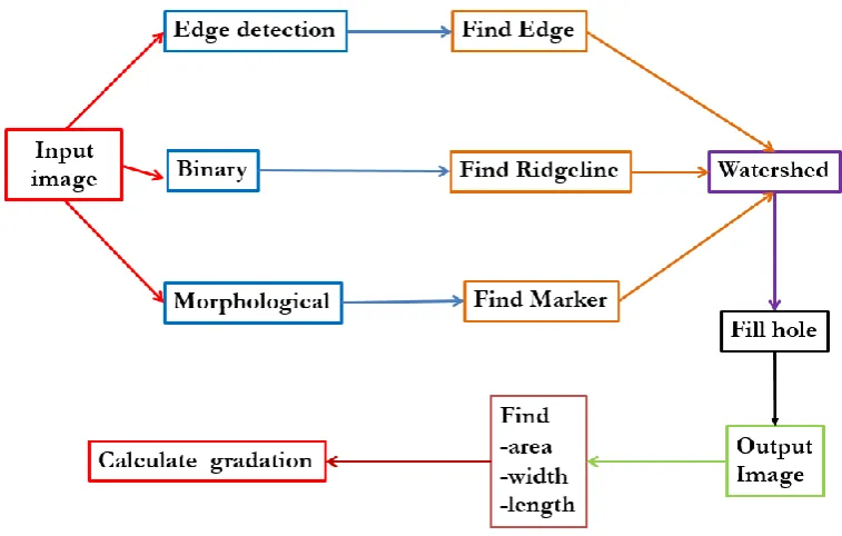
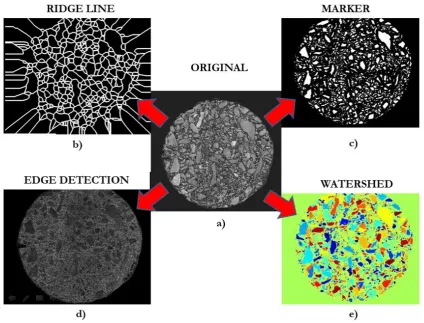
imaging. The edge detection is used to find the edges of the aggregate particles from their basic appearance, as shown in Fig. 2. The binary method is used to find ridge lines which separate aggregate territories, while the morphological segmentation is used to find markers of the approximate positions of aggregate particles. Afterwards, the image results from the three methods are received and are used later in the WT process to finally separate aggregate particles from the image background (Fig. 2e). The WT method is effective in the separation of connected aggregates and is widely used by many researchers [21-24]. The WT finds “catchment basins” and “watershed ridge lines” in the image by treating them as a surface where light pixels were high and dark pixels are low.

Fig. 2. (a) Image input, (b) ridge line, (c) marker, (d) image after edge detection and (e) WT segmentation.

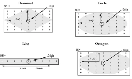
Fig. 3. Examples of shape structures used to fit the aggregate [25].

In the binary image output from the WT method, there was typically some noise found in the aggregate bodies (Fig. 4), which produced errors in identifying aggregate particles. Accordingly, the hole-filling technique [26, 27] was applied to eliminate these noises (Fig. 4). Afterwards, a particle image analysis was

used to use the pixels in the particle tocalculate the area, width, length and perimeter of each particle and to

count the number of particles.

Fig. 4. Examples of the hole-filling technique. (a) Image with noise before and (b) after (the output) the hole-filling technique.

2.2. Determining the Dimensional Properties of Aggregates

Fig. 5. Counting of aggregates.

Here Feret’s diameter[29] was applied to determine the dimension of each aggregate particle, where the

length is the maximum distance from one end to the other end of an aggregate particle and the width is the maximum distance that is perpendicular with the length from one end to the other end of the aggregate particle. The width of each aggregate particle was used to classify its sieve size (Fig. 6). If the width of the aggregate was smaller than the sieve size, it could pass that sieve. The area of an aggregate particle is calculated by counting the number of pixels (Fig. 7) and multiplying by the pixel unit size (mm/pixel).

Fig. 7. Measurement of area. The (a) actual area and (b) pixel area from computer [31].

3.

Problems Statement and Proposed Alternatives

However, some problems were commonly found in analyzing the process that can possibly lead to errors in

the aggregate geometry. Firstly, we found over-segmentation, where aggregates are separatedexcessively

into smaller particles than their actual sizes (Fig. 8b). This was caused by using too small a pixel value to fit various shapes of the aggregates. Secondly, we found under-segmentation, where aggregates were separated into larger particles than their actual sizes due to using too large a pixel value to fit the shapes of the aggregates (Fig. 8c).

Fig. 8. The (a) input image of the cross-section and the resulting (b) over segmentation and (c) under segmentation

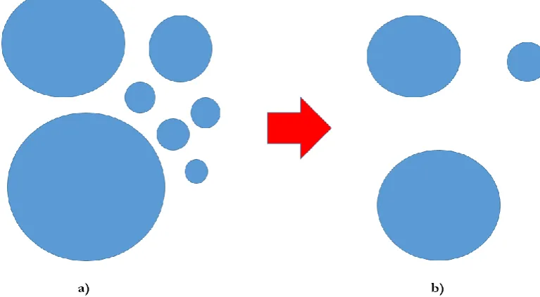
Lastly, we found the connected aggregate problem, in which some connected aggregate particles were identified as a single particle (Fig. 9). This problem affected the accurate counting of the number of particles.

a) b)

Fig. 9. Connected aggregate problem after WT segmentation.(a) Eight-bit greyscale image and (b) binary

image with WT segmentation

In this paper, two new methods to separate particles from their contact appearance are introduced.

These are the seven-layer overlaying (SLO)andsize-based multiple erosion (SBME) methods. In order to

evaluate their effectiveness in reducing errors, the results obtained from using the two methods were

compared with that obtained from manually separating the particles using photo editing software.

3.1. Method A: SLO

The SLO method begins with the two outputs of colored images produced from the WT method. The two colored images (Figs. 10a and b), which are different in their number of pixels specified in the WT method, were converted to binary (black and white) images and then the hole-filling technique was applied to the two binary images (Figs. 10c and d). Next, the white area of the hole-filled images was used to check the consistency of the two images. If the pixels in the two hole-filled images are both white at the same spot, the pixel color of the larger pixel image was assigned to the pixel on the smaller pixel image. The output image (Fig. 10e) was overlaid for layers number one and two. In the next step, the output image from the previous step was taken as the smaller pixel image to be compared with the next larger pixel colored image (layer 3). These steps were repeated until the colored images of seven different pixel sizes were processed, giving seven layers.

Fig. 10. The SLO method.

Fig. 11. Input image (#0), and each subsequent image layer processed by WT with a different number of pixels to result in seven layers (1–7#) and then form the final image (8#) after overlaying the seven layers.

3.2 Method B: SBME

In the SBME method, the erosion technique was used to solve the connected aggregate problem. After erosion, it was possible to separate the images of connected aggregates, as shown in Fig. 12. However, the problem of the erosion technique is that if the erosion is conducted with too large a pixel-value, images of small fragments of aggregates would then be completely eroded and disappear (Fig. 12b).

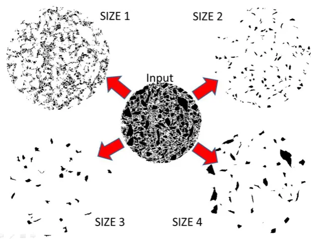
Given that different aggregate sizes would require different pixel-values to erode, then the input image was separated according to the aggregate sizes before the erosion. The separated images were then eroded with different pixel-values suitable for each aggregate size (see below).

This process started with the input image from an image scanner (Fig. 13a) and then underwent the WT technique using a diamond shape of 6-pixel size (Fig. 13b). The edges of fragments, which appear as a white colored pixel in the colored image, were detected and copied in a black colored binary image (Fig. 13c). The binary image with fragment edges was copied and then processed with the hole-filling technique (Fig. 13d), prior to separating into four images according to the four aggregate sizes (Fig. 13e) using pixel values of 1–10,000, 10,001–30,000, 30,001–50,000 and ≥ 50,001 (Fig. 14). Each separated image was then eroded with the preselected suitable pixel number for each aggregate size (Fig. 13f) of 4, 20, 30 and 60 pixels for the aggregates with 10,001–30,000, 30,001–50,000 and ≥ 50,001 pixels, respectively.

The images after the erosion technique were then used to calculate the area, width, length and perimeter of each aggregate. Although erosion was effective in separating connected aggregate images, it

reduced some aggregate areas, leading to an inaccurate calculation. Thus, theaggregate perimeter and area

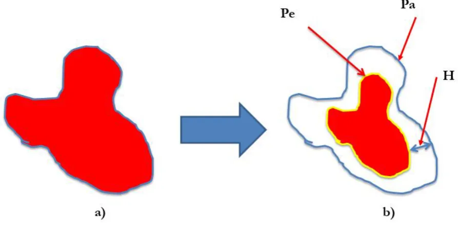
need some adjustment. Since the aggregate particle was reduced by the thickness of the number of eroded pixels times the unit pixel size (mm/pixel), its perimeter was first lengthened. The adjusted aggregate perimeter was calculated using Eqs. (2)–(4), based on the assumption in Fig. 15, where the adjusted area was calculated using Eq. (5).

Pe = 2 Re, (2)

Ra = Re + H, (3)

Pa = 2 Ra, (4)

Aa = Ae + Pa  H, (5)

where Pe is the perimeter of the eroded aggregate particle, Re is the equivalent radius of the eroded aggregate particle, H is the thickness of erosion, and is equal to the number of eroded pixels x unit pixel size (mm/pixel), Ra is the equivalent radius of the adjusted aggregate particle and Pa is the perimeter of the adjusted aggregate particle.

Fig. 15. Perimeter adjustment showing the particle (a) before and (b) after erosion.

4.

Verification of the Proposed Methods

Fig. 16. Creation of sectional image of an asphalt mixture cylinder. The (a) asphalt concrete sample, (b)

horizontal saw cut and (c)sectional image.

The asphalt mixture section was scanned to an 8-bit greyscale TIF file and all the connected aggregate particles in the image were separated manually using a photo editing software (Fig. 17). This image was then used as the reference in comparison with the results obtained from the SLO and SBME methods. The reference image was processed through the typical method for determining aggregates described earlier to obtain the referenced dimensions, areas and perimeters of aggregates for comparison.

Fig. 17. (a) Scanned image input and (b) after separating connected aggregates manually using photo editing software.

Fig. 18. Verification of the proposed methods.

The percent retained on sieve sizes [33] was the key index used to validate the effectiveness of the proposed methods. In the analysis, each aggregate particle volume could not be calculated since only a sectional area of the aggregate particle was available. Thus, a modified percent retained on sieve size by area was calculated using Eq. (6) to resemble the percent retained by weight definition [33];

%Retainedby area =

total n

i i

A

a



where ai is the aggregate image area of the particle,



n

i 1

a

of all particles retained in that sieve size and Atotal is the sectional area of the asphalt mixture.

5.

Results and Analysis

Table 1. Percent retained by area for each method.

Aggregate sieve size

(mm)

%Retained by area Error2

Manual SLO SBME WT SLO SBME WT

12.7 0 2.7 0 0 7.29 0 0

9.5 1.9 5.1 2.1 3.2 10.24 0.04 1.69

4.75 (#4) 13.7 16.9 17.1 17.5 10.24 11.56 14.44

2.38 (#8) 18.6 13.4 20.6 26.3 27.04 4.00 59.29

< 2.38 20.5 14.4 18.3 13.7 37.21 4.84 46.24

Sum 92.02 20.44 121.66

Fig. 19. Comparison of the percent retained of four methods: manual separation by photo editing software,

SLO, SBME and ordinary WT.

Table 2 Number of aggregate particles counted in the sectional image.

Sieve size

(mm) Amount of aggregate Error

2

Manual SLO SBME WT SLO SBME WT

12.7 0 1 0 0 1 0 0

9.5 1 4 1 3 9 0 4

4.75 (#4) 29 38 25 32 81 16 9

2.38 (#8) 113 91 113 102 484 0 121

< 2.38 832 580 824 750 63504 64 6724

Total 975 714 963 887 _{64079 80 6858}

they were found to be able to identify the aggregate particles more accurately than a normal WT method. The SBME method yielded the best results in identifying the number of aggregate particles and calculating the percent retained on each sieve size.

Although, the SBME method was able to provide more accurate identification of aggregate particles contained in a sectional image sample of HMA. However, applying the method as an acceptable alternative to the conventional sieving method still need further works to account on the key issues such as the real three-dimensional appearance of aggregate particles and the statistical evaluation of the new alternative method in comparison to the conventional sieving method. In the next stage, the authors plan to extend the verification of the new method by producing a number of sectional image analysis and laboratory sieved samples for statistical evaluation of the new and the conventional methods.

Acknowledgements

We would like to sincerely thank the 90th _{Anniversary of Chulalongkorn University Fund}

(Ratchadaphiseksomphot Endowment Fund), the Infrastructure Management Research Unit and Research and Researcher for Industry (RRI) of the Thailand Research Fund (TRF) for the financial support of this study.

References

[1] F. L. Roberts, P. S. Kandhal, E. R. Brown, D. Y. Lee, and T. W. Kennedy, “Aggregates,” in Hot Mix

Asphalt Materials, Mixture Design, and Construction, 2nd ed. Lanham, MD, USA: National Asphalt

Pavement Association Education Foundation, 1996, ch. 3, pp. 121-172.

[2] Pavement Interactive. (2007). Asphalt Binder and Characterization (13 August 2007). [Online]. Available:

http://www.pavementinteractive.org/article/asphalt-binder-and-characterization/ [Accessed: 7

October 2016]

[3] L. Bruno, G. Parla, and C. Celauro, “Image analysis for detecting aggregate gradation in asphalt

mixture from planar images,” Construction and Building Materials, vol. 28, no. 1, pp. 21-30, 2012.

[4] M. Vadood, M. S. Johari, and A. R. Rahaei, “Introducing a simple method to determine aggregate

gradation of hot mix asphalt using image processing,” International Journal of Pavement Engineering, vol. 15,

no. 2, pp. 142–150, 2013.

[5] F. S. Barbosa, M. C. R. Farage, A.-L. Beaucour, and S. Ortola, “Evaluation of aggregate gradation in

lightweight concrete via image processing,” Construction and Building Materials, vol. 29, pp. 7-11, 2012.

[6] A. K. H. Kwan, C. F. Mora, and H. C. Chan, “Particle shape analysis of coarse aggregate using digital

image processing,” Cement and Concrete Research, vol. 29, no. 9, pp. 1403–1410, 1999.

[7] Z. You, S. Adhikari, and M. E. Kutay, “Dynamic modulus simulation of the asphalt concrete using the

X-ray computed tomography images,” Materials and Structures, vol. 42, no. 5, pp. 617-628, 2009.

[8] I. S. Bessa, V. T. F. C. Branco, and J. B. Soares, “Evaluation of different digital image processing

software for aggregates and hot mix asphalt characterizations,” Construction and Building Materials, vol.

31, pp. 370-378, 2012.

[9] N. Chawla, R. S. Sidhu, and V. V. Ganesh, “Three-dimensional visualization and microstructure-based

modeling of deformation in particle-reinforced composites,” Acta Materialia, vol. 54, no. 6, pp.

1541-1548, 2006.

[10] Q. Guo, Y. Bian, L. Li, Y. Jiao, J. Tao, and C. Xiang, “Stereological estimation of aggregate gradation

using digital image of asphalt mixture,” Construction and Building Materials, vol. 94, pp. 458–466, 2015.

[11] Z. Q. Yue, W. Bekking, and I. Morin, “Application of digital image processing to quantitative study of

asphalt concrete microstructure,” Transportation Research Record, vol. 1492, pp. 53-60, 1995.

[12] E. Masad, B. Muhunthan, N. Shashidhar, and T. Harman, “Internal structure characterization of

asphalt concrete using image analysis,” Journal of Computing in Civil Engineering, vol. 13, no. 2, pp. 88-95,

1999.

[13] E. Masad, B. Muhunthan, N. Shashidhar, and T. Harman, “Quantifying laboratory compaction effects

on the internal structure of asphalt concrete,” Transportation Research Record: Journal of the Transportation

Research Board, vol. 1681, pp. 179-185, 1999.

[14] Z. Q. Yue and I. Morin, “Digital image processing for aggregate orientation in asphalt concrete

[15] G. R. Chehab, Y. R. Kim, R. A. Schapery, M. W. Witczak, and R. Bonaquist, “Characterization of asphalt concrete in uniaxial tension using a viscoelastoplastic continuum damage model,” Association of Asphalt Paving Technologists Technical Sessions, 2003, Lexington, Kentucky, USA, 2003, vol. 72.

[16] S. Kose, M. Guler, H. Bahia, and E. Masad, “Distribution of strains within hot-mix asphalt binders:

Applying imaging and finite-element techniques,” Transportation Research Record: Journal of the

Transportation Research Board, vol. 1728, pp. 21-27, 2000.

[17] H. M. Zelelew, A. T. Papagiannakis, and E. Masad, “Application of digital image processing

techniques for asphalt concrete mixture images,” in Proc. the 12th International Conference of International

Association for Computer Methods and Advances in Geomechanics (IACMAG), October 2008, pp. 119-124.

[18] A. Papagiannakis, A. Abbas, and E. Masad, “Micromechanical analysis of viscoelastic properties of

asphalt concretes,” Transportation Research Record: Journal of the Transportation Research Board, vol. 1789, pp.

113-120, 2002.

[19] H. Kim and W. G. Buttlar, “Discrete fracture modeling of asphalt concrete,” International Journal of

Solids and Structures, vol. 46, no. 13, pp. 2593-2604, 2009.

[20] Y. Liu and Z. You, “Visualization and simulation of asphalt concrete with randomly generated

three-dimensional models,” Journal of Computing in Civil Engineering, vol. 23, no. 6, pp. 340-347, 2009.

[21] H. J. Lee and Y. R. Kim, “Viscoelastic continuum damage model of asphalt concrete with healing,”

Journal of Engineering Mechanics, vol. 124, no. 11, pp. 1224-1232, 1998.

[22] W. Zhang, A. Drescher, and D. E. Newcomb, “Viscoelastic analysis of diametral compression of

asphalt concrete,” Journal of Engineering Mechanics, vol. 123, no. 6, pp. 596-603, 1997.

[23] J. Luca and D. Mrawira, “New measurement of thermal properties of superpave asphalt concrete,”

Journal of Materials in Civil Engineering, vol. 17, no. 1, pp. 72-79, 2005.

[24] J. K. Gilbert and J. C. Clausen. “Stormwater runoff quality and quantity from asphalt, paver, and

crushed stone driveways in Connecticut, “ Water research, vol. 40, no. 4, pp. 826-832, 2006.

[25] P. D. Kovesi, “MATLAB and Octave functions for computer vision and image processing,” Online:

https://www.mathworks.com/help/images/ref/strel-class.html, 2000.

[26] C. K. Chui and M. J. Lai, “Filling polygonal holes using C1 cubic triangular spline patches,” Computer

Aided Geometric Design, vol. 17, no. 4, pp. 297-307, 2000.

[27] Y. C. Fan and T. C. Chi, “The novel non-hole-filling approach of depth image based rendering,” in

3DTV Conference: The True Vision-Capture, Transmission and Display of 3D Video, 2008, pp. 325-328.

[28] M. D. Abràmoff, P. J. Magalhães, and S. J. Ram, “Image processing with ImageJ,” j. Biophotonics

International, vol. 11, no. 7, pp. 36-42, 2004.

[29] C. Y. Kuo, J. Frost, J. Lai, and L. Wang, “Three-dimensional image analysis of aggregate particles

from orthogonal projections,” Transportation Research Record: Journal of the Transportation Research Board,

vol. 1526, pp. 98-103, 1996.

[30] A. K. H. Kwan, C. F. Mora, and H. C. Chan. “Particle shape analysis of coarse aggregate using digital

image processing,” Cement and Concrete Research, vol. 29, no. 9, pp. 1403-1410, 1999.

[31] S. Levachkine, “Raster to vector conversion of color cartographic maps,” in International Workshop on

Graphics Recognition, Springer, Berlin, Heidelberg, 2003, pp. 50-62.

[32] S. Unsiwilai, “Influences of crumb rubber size in aggregate blend on deformation resistance properties

of hot mix asphalt,” M.Eng. thesis, Civil Eng. Dept., Chulalongkorn Univ., Bangkok, Thailand, 2013.

[33] Standard Test Method for Sieve Analysis of Fine and Coarse Aggregates, ASTM C136 / C136M-14, ASTM