Article
Interpolation-based Off-line Robust MPC for
Uncertain Polytopic Discrete-time Systems
Pornchai Bumroongsri
1,aand Soorathep Kheawhom
2,b,*
1 Department of Chemical Engineering, Faculty of Engineering, Mahidol University, Salaya, Nakhon Pathom 73170, Thailand
2 Computational Process Engineering, Department of Chemical Engineering, Faculty of Engineering, Chulalongkorn University, Phayathai Rd., Patumwan, Bangkok 10330, Thailand
E-mail: a[email protected], b[email protected] (Corresponding author)
Abstract. In this paper, interpolation-based off-line robust MPC for uncertain polytopic discrete-time systems is presented. Instead of solving an on-line optimization problem at each sampling time to find a state feedback gain, a sequence of state feedback gains is pre-computed off-line in order to reduce the on-line computational time. At each sampling time, the real-time state feedback gain is calculated by linear interpolation between the pre-computed state feedback gains. Three interpolation techniques are proposed. In the first technique, the smallest ellipsoids containing the measured state are approximated and the corresponding real-time state feedback gain is calculated. In the second technique, the pre-computed state feedback gains are interpolated in order to get the largest possible real-time state feedback gain while robust stability is still guaranteed. In the last technique, the real-time state feedback gain is calculated by minimizing the violation of the constraints of the adjacent inner ellipsoids so the real-time state feedback gain calculated has to regulate the state from the current ellipsoids to the adjacent inner ellipsoids as fast as possible. As compared to on-line robust MPC, the proposed techniques can significantly reduce on-line computational time while the same level of control performance is still ensured.
Keywords: Off-line robust MPC, linear interpolation, pre-computed state feedback gains.
ENGINEERING JOURNAL Volume 18 Issue 1
1.
Introduction
Model predictive control (MPC) has originated in the industry as an on-line computer control algorithm to solve multivariable control problems. At each sampling instant, MPC uses an explicit process model to solve the optimization problem and only the first computed input is implemented to the process. Although MPC has been successfully implemented to many industrial processes, it is well-known that stability of MPC cannot be guaranteed in the presence of model uncertainty [1]. For this reason, synthesis approaches for robust MPC have been widely investigated [2-6].
On-line robust MPC has been proposed by many researchers. Kothare et al. [2] proposed the algorithm that constructs an invariant ellipsoid containing the measured state at each sampling instant. Any states in this invariant ellipsoid can be driven to the origin by using the stabilizing state feedback gain. Thus, robust stability is guaranteed. The stabilizing state feedback gain is derived by using a single Lyapunov function so a certain degree of conservativeness is obtained. The conservativeness can be reduced by on-line robust MPC formulation using parameter-dependent Lyapunov function as proposed in [3-6]. However, the number of decision variables and constraints also increases. Thus, the algorithms are not suitable for relatively fast dynamic processes. Another approach to reduce the conservativeness is to increase the degrees of freedom in solving the optimization problem by adding a sequence of free control inputs to the state feedback control law [7-11]. By doing so, larger on-line computational time is required to calculate a sequence of free control inputs so the algorithms can only be implemented to slow dynamic processes.
In order to reduce on-line computational time, various researchers have studied off-line robust MPC [12-20]. Wan and Kothare [12] proposed an off-line robust MPC formulation using linear matrix inequalities (LMIs). The on-line computational time is reduced by pre-computing off-line a sequence of state feedback gains corresponding to a sequence of ellipsoidal invariant sets. At each sampling instant, the state is measured and the real-time state feedback gain is calculated by linear interpolation between the pre-computed state feedback gains. Although the on-line computational time is significantly reduced, a certain degree of conservativeness is obtained because the algorithm is derived by minimizing the worst-case performance cost. This strategy can be further improved by using the nominal performance cost as proposed by Ding et al. [13]. However, the approach in [13] is restricted to the case of a single Lyapunov function. Another idea is to incorporate the scheduling parameter into off-line MPC formulation. In [14], the sequences of state feedback gains corresponding to the sequences of ellipsoids are pre-computed off-line. At each sampling instant, the scheduling parameter is measured and the real-time state feedback gain is calculated by linear interpolation between the pre-computed state feedback gains of each sequence. Off-line robust MPC can also be formulated by using polyhedral invariant sets [15-20] in order to enlarge the size of stabilizable region. Later, an interpolation technique for polyhedral invariant sets was developed to reduce conservativeness and improve the control performances [21].
Recently, Bumroongsri and Kheawhom [22] have developed on-line robust MPC based on nominal performance cost by extending the results of Ding et al. [13] to the case of parameter-dependent Lyapunov function. However, the optimization problem solved at each sampling instant has many decision variables and constraints so its application is rather restricted to relatively slow dynamic processes. This algorithm was then further improved by off-line pre-computing a sequence of state feedback gains corresponding to the sequences of ellipsoidal invariant sets [23].
In this paper, the off-line robust MPC based on nominal performance cost for uncertain polytopic discrete-time systems [23] is further improved by implementing interpolation techniques. Three interpolation techniques are proposed. A sequence of state feedback gains is pre-computed off-line. At each sampling time, the real-time state feedback gain is calculated by linear interpolation between the pre-computed state feedback gains. The control performance of each technique is evaluated and compared within an example.
The paper is organized as follows. In section 2, the problem description is presented. In section 3, interpolation-based off-line robust MPC is presented. In section 4, we present an example to illustrate the implementation of the proposed algorithm. Finally, in section 5, we conclude the paper.
2.
Problem Description
) ( ) ( ) ( ) ( ) ( ) ( ) 1 ( k Cx k y k u k B k x k A k x (1)
where x(k) is the vector of states, u(k) is the vector of control inputs and y(k) is the vector of plant
outputs. Moreover, we assume that
]} , [ ],.., , [ ], , {[ , )] ( ), (
[Ak Bk Ω ΩCo A1 B1 A2 B2 AL BL (2)
where Ω is the polytope,
Co
denotes convex hull, [Aj,Bj] are the vertices of Ω and L is the number ofthe vertices of Ω. Any [A(k),B(k)] within the polytope is a linear combination of the vertices such that 1 0 , 1 ], , [ )] ( ), ( [ 1 1 j L j j j j L j j B A k B k
A (3)
where [1,2,...,L] is the uncertain parameter vector. The aim of this research is to find the state
feedback control law
) / ( ) /
(k i k Kxk i k
u (4)
which stabilizes the system (1) and minimizes the following nominal performance cost
) ( min , 0 ), /
(k i k i Jn k
u u(kmini/k),i0Jn,(k)
) / ( ) / ( 0 0 ) / ( ) / ( ^ 0 ^ , ( ) k i k u k i k x R k i k u k i k x T i n k
J (5)
where x^(ki/k) denotes the predicted nominal state, 0 and R0 are symmetric weighting matrices,
subject to input and output constraints
max ,
) /
( h
h k i k u
u ,h1,2,3,...,nu (6)
max ,
) /
( r
r k i k y
y ,r1,2,3,...,ny (7)
where nu is the number of control inputs and ny is the number of plant outputs.
In [22], the optimization problem (5) is formulated as the convex optimization involving linear matrix inequalities (LMIs). At each sampling time, the state feedback control law which minimizes the upper bound n on the nominal performance cost Jn,(k)and asymptotically stabilizes the closed-loop systems within the ellipsoids { / 1 1, 12,..., }
L , j x Q x x T j
j
is given by 1
), / ( ) /
(ki k Kxki k KYG
u where Y
and G are obtained by solving the following problem
γn Y,G,Qj min (8) L , j , Q k/k
x( ) j 0 12,...,
1
s.t.
(9) L , l L, , j , I γ Y R I γ G Θ Q Y B G A Q G G n n l ^ ^ j T ,..., 2 1 ,..., 2 1 0 0 0 0 2 1 2
1
(10) L , l L, , j , Q Y B G A Q G G l j j j T ,..., 2 1 ,..., 2 1
0
(11) u h, hh j T
T G G Q , j , L,X u ,h , , n
Y X ..., 2 1 ,..., 2 1
0 2max
(12) y r, rr j T T T j j n , , ,r y S L , j , Q G G C Y) B G (A S ..., 2 1 , ,..., 2 1
0 2max
where [A^,B^] denotes the nominal model of the plant, the symbol denotes the corresponding transpose
of the lower block part of symmetric matrices, I denotes the identity matrix, X is the diagonal matrix of
input constraints and S is the diagonal matrix of output constraints.
Robust stability is guaranteed by the Lyapunov stability constraint (10). For proof details, the reader is referred to [22]. Since the on-line optimization problem contains many decision variables and constraints, the algorithm requires large on-line computational time. Moreover, the number of constraints grows exponentially with the number of vertices of the polytope Ω.
3.
The Proposed Algorithm
In this section, interpolation-based off-line robust MPC for uncertain polytopic discrete-time systems is presented. The aim is to reduce the on-line computational burdens while the same level of control performance is still ensured. The on-line computational time is reduced by solving off-line the optimization problem (8) to find a sequence of state feedback gain Ki ,i1,2,...,Ncorresponding to the sequences of ellipsoids ,
x/x Qi,1jx1
T j
i
where i1,2,...,N is the number of ellipsoids and j1,2,...,L is the
number of vertices of polytope Ω. At each sampling time, the real-time state feedback gain is calculated by linear interpolation between the pre-computed state feedback gains.
3.1. Interpolation-Based Off-Line Robust MPC
Off-line: Choose a sequence of states xi,i1,2,...,N. For each xi, substitute x(k/k) in (9) by xi and
solve the optimization problem (8) to obtain the corresponding state feedback gain 1
i i
i YG
K and
ellipsoids ,
x/x Qi,1jx 1
, j 1,2,...,L.T j
i
Note that xi should be chosen such that i1,j i,j .
Moreover, for each iN, the following inequality must be satisfied ,1( 1) i,l1( j j i1)0,
T i j j j
i A B K Q A B K
Q
. 2 1 , 2
1, ....L l , ....L j
On-line: The real-time state feedback gain is calculated by linear interpolation between the pre-computed
state feedback gains. Three interpolation techniques are proposed as follows
Technique 1: The first technique is based on an approximation of the smallest ellipsoids containing the measured state. Instead of solving the optimization problem (8) at each sampling instant, the solution of the optimization problem (8) is approximated by finding the smallest ellipsoids containing the measured state. Then the corresponding real-time state feedback gain can be calculated by linear interpolation between the pre-computed state feedback gains. At each sampling time, when x(k)i,j ,x(k)i1,j,
N i L ... ,
j
12, , , , the real-time state feedback gain K((k))(k)Ki(1(k))Ki1 can be calculated from (k) obtained by solving the following problem.
) (
min k (14)
1 1
, 1,
s.t. ( ) ( ( )[x k T
k Qi j] (1
( ))[k Qi j]) ( ) 1, x k j 1 2,, .... L,
(15)
1 ) (
0 k (16)
It is seen that (k)0 and (k)1 correspond to the ellipsoids i1,j and i,j, respectively. Thus,
the smallest ellipsoids containing the measured state x(k) can be found by minimizing (k) in (14).
Moreover, it is seen that the optimization problem (14) is linear programming and the number of constraints grows only linearly with the number of vertices of the polytope Ω.
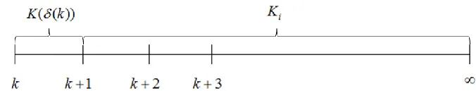
Figure 1 shows the graphical representation of the state feedback gain in each prediction horizon. It is seen that the same state feedback gain K((k))is implemented throughout the prediction horizon and
Fig.1. The graphical representation of the state feedback gain in each prediction horizon of technique 1.
Technique 2: In the second technique, the pre-computed state feedback gains Ki,i1,2,...,N are
interpolated in order to get the largest possible real-time state feedback gain. Since the pre-computed state feedback gains are larger as i increases, when the measured state lies between i,j and i1,j, this technique
tries to use the value of Ki1 as much as possible in the interpolation. This technique can implement larger
real-time state feedback gain compared to technique 1 so faster response is obtained. At each sampling time, when x(k)i,j ,x(k)i1,j, j1,2,...,L ,iN
,
the real-time state feedback gain K((k))(k)Ki(1(k))Ki1 can be calculated from (k) obtained by solving the following problem.) (
min k (17)
s.t. j L
Q k x k K B A k x k K B A j i j j T j
j 0, 1,2,...,
) ( ))) ( ( ( )) ( ))) ( ( (( 1 , (18) 0 1 )) ( )) ( ( ( 2 max , h h k x k K u
(19)
1 ) (
0 k (20)
1
i
K is always larger than Ki because input and output constraints impose less limit on the state
feedback gain as i increases. Thus, the largest possible real-time state feedback gain
1 )) ( 1 ( ) ( )) (
( k k Ki k Ki
K can be calculated by minimizing (k) in (17). The next predicted state
is restricted to lie in the ellipsoidal invariant set by (18) so robust stability is still guaranteed. The input constraint is guaranteed by (19). Note that the output constraint does not need to be incorporated into the problem formulation because the satisfaction of (18) also guarantees output constraint satisfaction. It is seen that the optimization problem (17) is formulated as the convex optimization involving linear matrix inequalities (LMIs) and the number of constraints grows only linearly with the number of vertices of the polytope Ω.
Figure 2 shows the graphical representation of the state feedback gain in each prediction horizon. It is seen that the largest possible real-time state feedback gain K((k))is only implemented at each sampling
time k. At time k1 and so on, the state feedback gain Ki is implemented. Thus, the state must be
restricted to lie in the ellipsoids i,j and robust stability is guaranteed.
Fig.2. The graphical representation of the state feedback gain in each prediction horizon of technique 2.
j i1,
, the real-time state feedback gain calculated has to drive the state from i,j to i1,j as fast as
possible in order to minimize the violation of the constraints of i1,j. At each sampling time, when
N i L ... , j k x k
x( )i,j, ( )i1,j, 12, , , , the real-time state feedback gain
1 )) ( 1 ( ) ( )) (
( k k Ki k Ki
K can be calculated from (k) obtained by solving the following problem.
) (
min k (21)
s.t. j L
Q k x k K B A k x k K B A k j i j j T j j ,..., 2 , 1 , 0 ) ( ))) ( ( ( )) ( ))) ( ( (( ) ( 1 , 1 (22) L j Q k x k K B A k x k K B A j i j j T j j ,..., 2 , 1 , 0 ) ( ))) ( ( ( )) ( ))) ( ( (( 1 , (23) 0 1 )) ( )) ( ( ( 2 max , h h k x k K u
(24)
1 ) (
0 k (25)
By applying Schur complement to (22), we obtain x (k 1) Qi11,jxj(k 1) 1 (k)
T
j where
) ( ))) ( ( ( ) 1
(k A B K k xk
xj j j . By minimizing (k) in (21), the real-time state feedback gain
1 )) ( 1 ( ) ( )) (
( k k Ki k Ki
K calculated has to regulate the state from the current ellipsoids i,j to the
adjacent inner ellipsoids i1,j as fast as possible. The next predicted state is restricted to lie in the
ellipsoidal invariant set by (23) so robust stability is still guaranteed. The input constraint is guaranteed by (24). Note that the output constraint does not need to be incorporated into the problem formulation because the satisfaction of (23) also guarantees output constraint satisfaction. It is seen that the optimization problem (21) is formulated as the convex optimization involving linear matrix inequalities (LMIs) and the number of constraints grows only linearly with the number of vertices of the polytope Ω.
Figure 3 shows the graphical representation of the state feedback gain in each prediction horizon. It is seen that the real-time state feedback gain calculated K((k)) is only implemented at each sampling time k.
At time k1 and so on, the state feedback gain Ki is implemented. Thus, the state must be restricted to lie
in the ellipsoids i,j and robust stability is guaranteed.
Fig. 3. The graphical representation of the state feedback gain in each prediction horizon of technique 3.
4.
Example
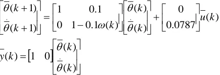
[image:6.596.127.465.566.631.2]) ( 0787 . 0 0 ) ( ) ( ) ( 1 . 0 1 0 1 . 0 1 ) 1 ( ) 1 ( .
. u k
k k k k k
) ( ) ( 0 1 ) ( . k k k y (26)
where (k) is the angular position of the antenna, ( )
.
k
is the angular velocity of the antenna and u(k) is
the input voltage to the motor. The uncertain parameter
(k) is proportional to the coefficient of viscous friction in the rotating parts of the antenna. It is assumed to be arbitrarily time-varying in the range of10 ) ( 1 .
0 k . Since the uncertain parameter
(k) is varied between 0.1 and 10, we conclude thatΩ k
A( ) where Ω is given as follows
0 0 1 . 0 1 , 99 . 0 0 1 . 0 1 Co
Ω
(27)
The objective is to regulate to the origin by manipulating u. The input constraint is u(k) 2volts.
Here Jn,(k) is given by (5) with
0 0 0 1
[image:7.596.226.451.82.159.2]Θ and R0.00002.
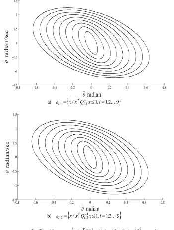
Figure 4 shows two sequences of ellipsoids ,
x/x Qi,1jx 1,i 1,2,...,9,j 1,2
T j
i
constructed off-line.
Note that the ellipsoids are constructed such that i1,j i,j. In this example, two sequences of ellipsoids
/ 1, 12 9
a) i,1 x xTQi,11x i , ,...,
/ 1, 12 9
b) i,2 x xTQi,21x i , ,...,
Fig. 4. Two sequences of ellipsoids ,
x/x Qi,1jx 1,i 1,2,...,9,j 1,2
T j
i
, each sequence has 9
ellipsoids.
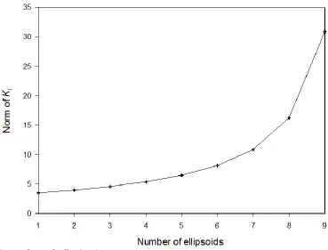
Figure 5 shows norm of state feedback gains Ki,i1,2,...,9. It is seen that norm of Kiincreases as i
increases. This is due to the fact that input constraint imposes less limit on the state feedback gain as i
[image:8.596.129.480.82.545.2]Fig. 5. Norm of state feedback gains Ki,i1,2,...,9.
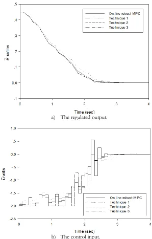
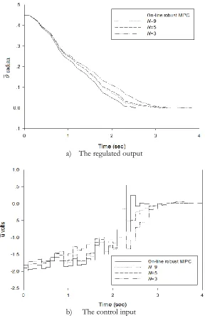
Figure 6 shows the closed-loop responses of the system when (k) is randomly time-varying between 10
) ( 1 .
0 k . As compare to on-line robust MPC [22], technique 1 gives slower response because the
real-time state feedback gain and the ellipsoids calculated in technique 1 are only approximations of those calculated by solving on-line optimization problem (8). In comparison, technique 2 and technique 3 give faster responses than technique 1 because they are based on ideas that are completely different from technique 1. In technique 2, the pre-computed state feedback gains are interpolated to get the largest possible real-time state feedback gain so technique 2 tends to make the process responses less sluggish than technique 1. In technique 3, the real-time state feedback gain calculated has to regulate the state from the current ellipsoids i,j to the adjacent inner ellipsoids i1,j as fast as possible in order to minimize the
[image:9.596.114.483.80.361.2]a) The regulated output.
b) The control input.
Fig. 6. The closed-loop responses of the system when (k) is randomly time-varying between 10
) ( 1 .
0 k ; a) The regulated output; b) The control input.
[image:10.596.148.446.76.543.2]
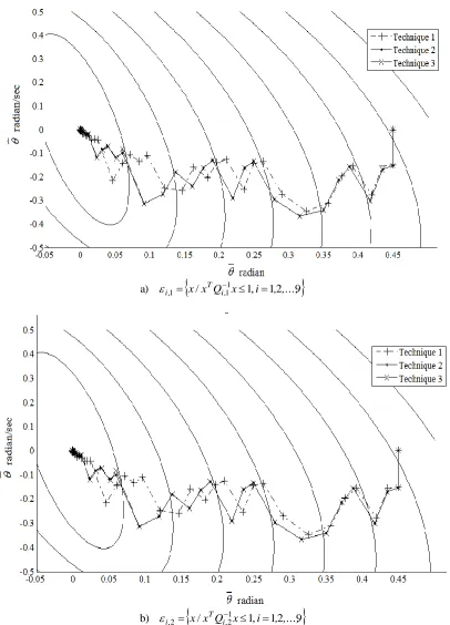
/ 1, 12 9
a) i,1 x xTQi,11x i , ,...,
/ 1, 12 9
b) i,2 x xTQi,21x i , ,...,
Fig. 7. The state trajectories: a) i,1; b) i,2.
[image:11.596.98.504.77.641.2]Table 1. The on-line computational time at each sampling instant.
Algorithms On-line computational time (s)
On-line robust MPC [17] 0.213
Technique 1 0.001
Technique 2 0.047
Technique 3 0.101
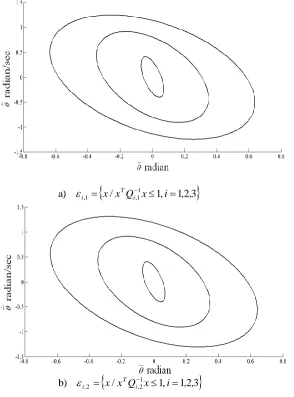
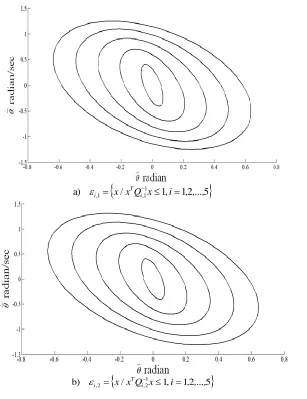
Next, the effect of the number of ellipsoids constructed off-line is investigated. Figures 8 and 9 show the sequences of ellipsoids when the number of ellipsoids constructed off-line is varied from 9 in Fig. 4 to 3 and 5, respectively. Less computer memory is required as the number of ellipsoids constructed off-line is decreased. Note that in the construction of ellipsoids, the inequality ,1( 1) i,l1( j j i1)0,
T i j j j
i A B K Q A B K
Q ....L
, l ....L ,
j12 , 12
must be satisfied. This inequality tends to be violated if the number of ellipsoids constructed off-line is too small.
/ 1, 123
a) 1
1 , 1
, x x Qi x i , ,
T
i
/ 1, 123
b) ,2 x x Qi,21x i , ,
T
i
Fig. 8. Two sequences of ellipsoids ,
x/x Qi,1jx 1,i 1,2,3,j 1,2
T j
i
[image:12.596.155.443.93.155.2] [image:12.596.156.450.266.663.2]
/ 1 , 12 5
a) ,1 x xQi,11x i , ,...,
T
i
/ 1, 12 5
b) 1
2 , 2
, x xQi x i , ,...,
T
i
Fig. 9. Two sequences of ellipsoids
/ 1 1, 12...5 12
,
, x x Qijx i , , , j ,
T j
i
, each sequence has 5
ellipsoids.
[image:13.596.156.463.76.475.2]a) The regulated output
b) The control input
Fig. 10. The closed-loop responses of technique 1 when the number of ellipsoids constructed off-line is varied from 3, 5 and 9; a) The regulated output; b) The control input.
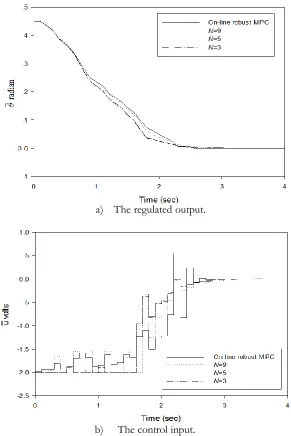
Figure 11 shows the closed-loop responses of technique 2 when the number of ellipsoids constructed off-line is varied from 3, 5 and 9. Since Ki1 is larger than Ki as shown in Fig. 5, larger real-time state
[image:14.596.156.444.78.522.2]a) The regulated output.
b) The control input.
Fig. 11. The closed-loop responses of technique 2 when the number of ellipsoids constructed off-line is varied from 3, 5 and 9; a) The regulated output; b) The control input.
Figure 12 shows the closed-loop responses of technique 3 when the number of ellipsoids constructed off-line is varied from 3, 5 and 9. The real-time state feedback gain calculated has to regulate the state from the current ellipsoids i,j to the adjacent inner ellipsoids i1,j as fast as possible in order to minimize the
violation of the constraints of i1,j. As the number of ellipsoids is decreased, i1,j are closer to the
[image:15.596.153.444.78.514.2]a) The regulated output.
b) The control input.
Fig. 12. The closed-loop responses of technique 3 when the number of ellipsoids constructed off-line is varied from 3, 5 and 9: a) The regulated output; b) The control input.
5.
Conclusions
This paper presents interpolation-based off-line robust MPC for uncertain polytopic discrete-time systems. The algorithm pre-computes off-line a sequence of state feedback gains corresponding to the sequences of ellipsoids. At each sampling time, the real-time state feedback gain is calculated by linear interpolation between the pre-computed state feedback gains. Three interpolation techniques are proposed. As compared to on-line robust MPC, the on-line computational time is significantly reduced while the same level of control performance is still ensured.
Acknowledgement
[image:16.596.157.446.75.532.2]References
[1] M. Morari and J. H. Lee, “Model predictive control: past, present and future,” Comput. Chem. Eng., vol. 23, pp. 667-682, 1999.
[2] M. V. Kothare, V. Balakrishnan, and M. Morari, “Robust constrained model predictive control using linear matrix inequalities,” Automatica, vol. 32, pp. 1361-1379, 1996.
[3] F. A. Cuzzola, J. C. Geromel, and M. Morari, “An improved approach for constrained robust model predictive control,” Automatica, vol. 38, pp. 1183-1189, 2002.
[4] W. J. Mao, “Robust stabilization of uncertain time-varying discrete systems and comments on “an improved approach for constrained robust model predictive control”,” Automatica, vol. 39, pp. 1109-1112, 2003.
[5] T. A. T. Do and D. Banjerdpongchai, “Robust constrained model predictive control for uncertain linear time-varying systems using multiple Lyapunov functions,” in Proceedings of SICE-ICASE International Joint Conference, Korea, 2006, pp. 908-913.
[6] N. Wada, K. Saito, and M. Saeki, “Model predictive control for linear parameter varying systems using parameter dependent Lyapunov function,” IEEE T. Circuits Syst., vol. 53, pp. 1446-1450, 2006. [7] J. Schuurmans and J. A. Rossiter, “Robust predictive control using tight sets of predicted states,” IEE
P.-Contr. Theor. Ap., vol.147, pp. 13-18, 2000.
[8] P. Bumroongsri and S. Kheawhom, “MPC for LPV systems based on parameter-dependent Lyapunov function with perturbation on control input strategy,” Engineering Journal, vol. 16, pp. 61-72, 2012. doi: 10.4186/ej.2012.16.2.61
[9] P. Bumroongsri and S. Kheawhom, “MPC for LPV systems using perturbation on control input strategy,” Computer Aided Chemical Engineering, vol. 31, pp. 350-354, 2012. doi: 10.1016/B978-0-444-59507-2.50062-7
[10] P. Bumroongsri and S. Kheawhom, “Improving the performance of robust MPC using the perturbation on control input strategy based on nominal performance cost,” Procedia Engineering, vol. 42, pp. 1027-1037, 2012. doi:10.1016/j.proeng.2012.07.494
[11] A. Casavola, D. Famularo, and G. Franze, “A feedback min-max MPC algorithm for LPV systems subject to bounded rates of change of parameters,” IEEE T. Automat. Contr., vol. 47, pp. 1147-1152, 2002.
[12] Z. Wan and M. V. Kothare, “An efficient off-line formulation of robust model predictive control using linear matrix inequalities,” Automatica, vol. 39, pp. 837-846, 2003.
[13] B. Ding, Y. Xi, M. T. Cychowski, and T. O. Mahony, “Improving off-line approach to robust MPC based-on nominal performance cost,” Automatica, vol. 43, pp. 158-163, 2007.
[14] P. Bumroongsri and S. Kheawhom, “An ellipsoidal off-line model predictive control strategy for linear parameter varying systems with applications in chemical processes,” Syst. Control Lett., vol. 61, pp. 435-442, 2012. doi:10.1016/j.sysconle.2012.01.003
[15] P. Bumroongsri and S. Kheawhom, “An off-line robust MPC algorithm for uncertain polytopic discrete-time systems using polyhedral invariant sets,” J. Process Contr., vol. 22, pp. 975-983, 2012. doi: 10.1016/j.jprocont.2012.05.002
[16] P. Bumroongsri and S. Kheawhom, “The polyhedral off-line robust model predictive control strategy for uncertain polytopic discrete-time systems,” IFAC Papersonline Advanced Control of Chemical Processes, vol. 8, pp. 655-660, 2012. doi:10.3182/20120710-4-SG-2026.00017
[17] P. Bumroongsri and S. Kheawhom, “A polyhedral off-line robust MPC strategy for uncertain polytopic discrete-time systems,” Engineering Journal, vol. 16, pp. 73-89, 2012. doi: 10.4186/ej.2012.16.4 [18] B. Pluymers, J. A. Rossiter, J. A. K. Suykens, and B. D. Moor, “Interpolation based MPC for LPV systems using polyhedral invariant sets,” in Proceedings of American Control Conference, vol. 2, 2005, pp. 810-815.
[19] B. Pluymers, J. A. Rossiter, J. A. K. Suykens, and B. D. Moor, “The efficient computation of polyhedral invariant sets for linear systems with polytopic uncertainty,” inProceedings of American Control Conference, vol. 2, 2005, pp. 804-809.
[20] J. A. Rossiter, B. Kouvaritakis, and M. Bacic, “Interpolation based computationally efficient predictive control,” Int. J. Control, vol. 77, pp. 290-301, 2004.
[22] P. Bumroongsri and S. Kheawhom, “Robust constrained MPC based on nominal performance cost with applications in chemical processes,” Procedia Engineering, vol. 42, pp. 1561-1571, 2012. doi: 10.1016/j.proeng.2012.07.549
[23] P. Bumroongsri and S. Kheawhom, “An ellipsoidal off-line robust model predictive control strategy for uncertain polytopic discrete-time systems,” IFAC PapersonlineControl Applications of Optimization, vol. 15, pp. 268-273, 2012. doi:10.3182/20120913-4-IT-4027.00018
[24] J. F. Sturm, “Using Sedumi 1.02, a MATLAB toolbox for optimization over symmetric cones,” Optim. Method Softw., vol. 11, pp. 625-653, 1999.
[25] J. Löfberg, “YALMIP: A toolbox for modelling and optimization in MATLAB,” inProceedings of the 2004 IEEE international symposium on computer aided control systems design, Taipei, Taiwan, 2004, pp. 284-289.