Development and verification of semi-blind receiver structures for broadband wireless communication systems

(1)

Development and Verification of Semi-Blind Receiver

Structures for Broadband Wireless Communication

Systems

Thesis submitted in accordance with the requirements of the University of Liverpool for the degree of Master in Philosophy

by

Teng Ma

(2)

Declaration

The work in this thesis is based on research carried out at the University of Liverpool.

(3)

Abstract

The increasingly high demands for high data rate wireless communication services

re-quire spectrum- and energy-efficient solutions. In this thesis, a number of energy-efficient semi-blind receiver structures are proposed to perform Doppler spread

estima-tion, channel estimation and equalisation for broadband wireless orthogonal frequency

division multiplexing (OFDM) systems. A real-time wireless communication testbed is developed to verify the proposed semi-blind receiver structures.

In the first contribution, a semi-blind Doppler spread estimation and Kalman filter-ing based channel estimation approach is proposed for wireless OFDM systems. A short

sequence of reference data is carefully designed and applied as pilot symbols for Doppler

spread estimation and channel estimation initialisation of the Kalman filter. Then the estimates of inter-carrier interference (ICI) caused by Doppler spread are gathered into

the equivalent channel model and compensated for through channel equalisation, which

dramatically reduces the computational complexity. The simulation results show that the proposed approach outperforms the conventional pilot aided Doppler spread and

channel estimation schemes.

In the second contribution, a semi-blind Doppler spread estimation and independent

component analysis (ICA) based equalisation scheme aided by non-redundant precoding

is proposed for wireless multiple-input multiple-output (MIMO) OFDM systems. A number of reference data sequences are selected from a pool of orthogonal sequences

for two purposes. First, the reference data sequences are superimposed in the source

data sequences through non-redundant linear precoding to enable the Doppler spread estimation by minimising the sum cross-correlation between the compensated signals

(4)

sequences are applied to eliminate the phase and permutation ambiguity in the ICA

equalised signals. Simulation results show that the proposed semi-blind MIMO OFDM system can achieve a bit error rate (BER) performance which is close to the ideal case

with perfect channel state information (CSI).

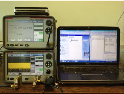
In the third contribution, a real-time wireless communication testbed is developed with a vector signal generator, a vector signal analyser and a pair of antennas, to

verify the effectiveness of the proposed receiver structures over the air in different environments such as Reverberation chamber and office area. Measurement results

show a good match with simulation results. Also, a pilot is employed for three purposes

(5)

Acknowledgement

First, I would like to express my deepest gratitude to Dr. Xu Zhu for teaching me

so much about research skills. This work benefits from her patient guidance, constant encouragement and invaluable comments during the period of my study in U.K.. I also

appreciate concerns from Prof. Yi Huang for my research. This thesis would not have

been completed without loads of support and help from them.

I would like to thank the University of Liverpool, as well as the Department of

Electrical Engineering and Electronics, for providing outstanding training and facilities to research students.

I would also like to thank my colleagues in the Wireless communication and Smart

Grid Group: Dr. Yufei Jiang for inspiring discussion and sharing research ideas with me, Dr. Linhao Dong for his support and encouragement, Mr. Chao Zhang, Mr.

Qinyuan Qian, Mr. Yanghao Wang, Mr. Kainan Zhu, Mr. Yang Li, Mr. Jun Yin,

Mr. Chaowei Liu, Mr. Zhongxiang Wei and Mr. Heggo Mohammad for creating a family-like atmosphere in the lab where I have been working. I was a pleasure to share

my good times with you.

Finally, my gratitude is dedicated to my parents. I would had no chance to pursue

my goals in my life without their support, patience and encouragement.

(6)

List of Figures

2.1 Fading channel types . . . 19

2.2 A typical Rayleigh fading channel impulse response . . . 20

2.3 Wireless OFDM system model block diagram . . . 22

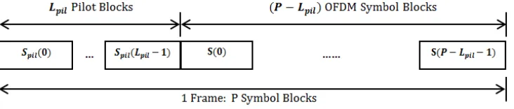
3.1 Proposed Kalman Filtering based Frame Structure . . . 42

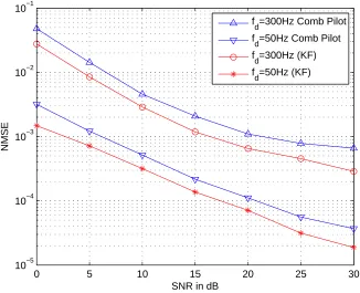
3.2 NMSE performance of the semi-blind Doppler spread Estimation in OFDM systems . . . 48

3.3 BER vs. Pilot overhead of the semi-blind Doppler spread tracking and Kalman filtering based channel estimation of OFDM systems . . . 49

3.4 BER vs. SNR in dB performance of semi-blind Doppler spread tracking and Kalman filtering based channel estimation of OFDM systems . . . . 51

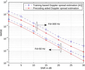
4.1 NMSE performance of the proposed semi-blind Doppler spread estima-tion in MIMO OFDM systems . . . 64

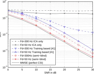
4.2 BER vs. SNR in dB performance of semi-blind Doppler spread estima-tion and ICA based equalizaestima-tion of MIMO OFDM systems . . . 65

5.1 The real-time wireless communication systems test-bed . . . 71

5.2 The Reverberation chamber at the University of Liverpool . . . 75

5.3 BER vs. precoding constant in room with SNR (dB)=30 dB . . . 78

5.4 BER vs. SNR (dB) in room area with precoding constanta= 0.36 . . . 79

5.5 BER vs. frame length in room area witha= 0.36, SNR (dB)=30 dB . . 79

5.6 Time domain received signal frame structure . . . 81

5.7 Proposed pilot structure with nulled CP . . . 81

(10)

5.9 Doppler spread spectrum in room with electrical fan . . . 85

5.10 Measurement of Doppler spread spectrum in room with electrical fan speed 0 (0 m/s) . . . 86

5.11 Measurement of Doppler spread spectrum in room with electrical fan

speed 1 (15.0 m/s) . . . 86 5.12 Measurement of Doppler spread spectrum in room with electrical fan

speed 2 (17.0 m/s) . . . 87 5.13 Measurement of Doppler spread spectrum in room with electrical fan

speed 3 (21.5 m/s) . . . 87

5.14 Doppler spread spectrum in Reverberation Chamber with electrical fan 88 5.15 Measurement of Doppler spread spectrum in Reverberation Chamber

with electrical fan speed 0 (0 m/s) . . . 88

5.16 Measurement of Doppler spread spectrum in Reverberation Chamber with electrical fan speed 1 (15.0 m/s) . . . 89

5.17 Measurement of Doppler spread spectrum in Reverberation Chamber with electrical fan speed 2 (17.0 m/s) . . . 89

5.18 Measurement of Doppler spread spectrum in Reverberation Chamber

with electrical fan speed 3 (21.5 m/s) . . . 90 5.19 BER vs. SNR in dB for Kalman filtering channel estimation approach

in room . . . 91

(11)

List of Tables

2.1 Evolution of Mobile Telephony Standards and Technologies . . . 10

2.2 Path Loss Exponent Values in Different Environments . . . 12 2.3 Fading Types . . . 18

5.1 Electrical Fan Speed Measurement Results and Coherence Time Calcu-lation . . . 83

(12)

Abbreviations and Acronyms

3G Third Generation

3GPP Third Generation Partnership Project

4G Fourth Generation

5G Fifth Generation

AWGN Additive White Gaussian Noise

BER Bit Error Rate

BSS Blind Source Separation

CAZAC Constant Amplitude Zero Auto-Correlation

CDMA Code-division Multiple Access

CFO Carrier Frequency Offset

CIR Channel Impulse Response

CP Cyclic Prefix

CPI Cyclic Prefix Insertion

CPR Cyclic Prefix Removal

CSI Channel State Information

DL Downlink

(13)

EDGE Enhanced Data Rates for GSM Evolution

FDE Frequency Domain Equalisation

FDM Frequency Division Multiplexing

FDMA Frequency Division Multiplexing Access

FFT Fast Fourier Transform

GSM Global System Mobile

HOS High Order Statistics

HSPA High Speed Packet Access

IBI Inter-Block Interference

ICI Inter-Carrier Interference

ICA Independent Component Analysis

IDFT Inverse Discrete Fourier Transform

IFFT Inverse Fast Fourier Transform

i.i.d. Independent Identically Distributed

I/Q Inphase/Quadrature

ISI Inter-Symbol Interference

JADE Joint Approximate Diagonalisation of Eigenmatrices

LO Local Oscillators

LOS Line-of-Sight

LS Least Square

LTE Long Term Evolution

(14)

ML Maximum Likelihood

MMSE Minimum Mean Square Error

MSE Mean Square Error

NMSE Normalised Mean Square Error

OFDM Orthogonal Frequency Division Multiplexing

OFDMA Orthogonal Frequency Division Multiple Access

PAPR Peak-to-Average Power Ratio

PL Path Loss

PDF Probability Density Function

PDP Power Delay Profile

RMS Root Mean Square

SC-FDMA Single-Carrier FDMA

SISO Single-Input Single-Output

SNR Signal-to-Noise Ratio

SOS Second Order Statistics

TDD Time Division Duplexing

TDMA Time Division Multiple Access

UL Uplink

UMTS Universal Mobile Telecommunications System

WiMAX Worldwide Interoperability for Microwave Access

(15)

Chapter 1

Introduction

1.1 Background

Wireless communications is, by any measure, a dynamic and broad field that has

ex-perienced the fastest grouth in the communication industry over the past few decades

[1, 2]. The demands for high-data-rate services allow amounts of research activities carried out for promoting a higher system capacity. In order to serve the purpose, a

number of wireless communication systems have been proposed and exploited. By

util-ising multiple transmit and receive antennas, Multiple-input multiple-output (MIMO) systems [3] becomes the dominant wireless communication technology, which can

pro-vide considerable channel capacity improvement than the systems with single-input single-output (SISO).

Orthogonal frequency division multiplexing (OFDM) technology was first proposed

in 1960 [4]. It is robust against frequency selective fading channels. By dividing the frequency selective fading channel into a number of parallel flat fading sub-channels,

the spatial diversity gain can be obtained. Due to the rapid development of digi-tal signal processing, this technology becomes practically possible and attractive to

the modern wireless communication systems. So far, OFDM has been employed in a

range of modern wireless communication systems. A well known technique, Long Term Evolution-Advanced (LTE-A) [5], is well developed and utilised in fourth generation

(4G) technologies.

(16)

transmitted. The equaliser coefficients are required, which can usually be obtained

di-rectly from channel state information (CSI). In wireless communication systems, based on some traditional methods, a number of reference data sequences regarded as training

signals are commonly applied to estimate the CSI before equalisation at the receiver.

However, the transmission of training signals not only consumes additional transmit power but also reduces the spectral efficiency. In order to recover source signal, blind or

semi-blind channel estimation and equalisation techniques [7] was proposed to obtain the CSI. Without consuming extra transmit power and spectral resource, the source

data can be recovered by employing the reference data sequences directly from the

statistics and structure of the received data sequences. As it requires non or only a little prior information in advance at the receiver, blind or semi-blind equalisation

technologies can improve spectral and power efficiency. The aim of this thesis is to

de-velop a real time measurement testbed and verify a number of energy efficient receiver structures in wireless communication systems over frequency selective channels.

In modern wireless communication systems, high mobility between transmit and receive antennas results in Doppler shift, which leads to time variate [8, 9] channel. In

mobile OFDM systems, the orthogonality among subcarriers can be destroyed by the

time variation, which accompanied with power leakage in OFDM subchannels. This phenomenon is known as inter-channel or inter-carrier interference (ICI) [10, 11, 12].

ICI, if not mitigated, could introduce ignorable system degradation and error floor

that will increase while Doppler spread is getting large. Consequently, the estimation of channel and channel parameters, such as Doppler spread, as well as channel

equalisa-tion are becoming important aspects while designing a wireless OFDM communicaequalisa-tion system. In the future wireless communication systems, support of mobility feature is

considered as one of the most critical characteristics. In many modern and future

wire-less communication systems, OFDM aided with the ability that can combat rapid time varying fading channels is deeply needed.

The Kalman filter [13] is known as a linear quadratic estimation technique. It is

(17)

ac-quires the previous measurement state information from unknown variables and then

update the estimates, which is much more precise than that of single measurement and estimation method. Formally, the Kalman filter is regarded as a recursive and optimal

estimator which obtain the estimates on streams of input noisy and uncertain signal

sequences in order to process and update a statistically optimised estimates. Further-more, it is considered and employed as an ideal technique in time domain estimation

and signal analysis, for instance, signal processing [14]. In order to adaptively track the channel variations of wireless communication, Kalman filtering based channel

esti-mation [15] was proposed for frequency selective fading channels systems. This kind of

channel estimation method is an efficient method as it requires only limited number of reference data to obtain the CSI even in time-varying channel.

Among those high order statistics (HOS) based techniques, independent component

analysis (ICA) [16] is considered as an high efficient blind source separation (BSS) technology [17]. It can recover the source data by maximising the non-Gaussianity

of the observed signals. Compared to the Second order statistics (SOS) based blind approaches [18], ICA potentially reduces the system sensitivity to noise. It is because

that the cumulates of the Gaussian noise in fourth or higher order are tending to be

zero. The ICA technique is applied to separate and recover the statistical independent components from the received data. So far, ICA has been used in a number of fields,

including signal separation in audio applications or brain imaging, analysis of economic

data and feature extraction [16]. The advantage of applying ICA is that it requires no CSI while performing blind or semi-blind equalisation. To improve the spectral

efficiency, ICA is employed in this thesis to do equalisation in simulation and the real-time OFDM wireless communication systems.

1.2 Research Contributions

The research conducted during the MPhil study has produced the following main con-tributions:

(18)

estima-tion approach is proposed for single-input single-output (SISO) OFDM systems,

where a short sequences of reference data are carefully designed and employed as the pilot for Doppler spread estimation and Kalman filtering channel

estima-tion initialisaestima-tion. The estimates of inter-carrier interference (ICI) introduced

by Doppler spread is gathered into the equivalent system model and mitigated through the equalisation process, which dramatically reduces the system

compu-tational complexity. According to the simulation results, it can be demonstrated that the proposed estimation approach can outperform the conventional comb

type pilot aided estimation methods in bit error rate (BER).

• A semi-blind receiver structure is proposed for MIMO OFDM systems, with a precoding aided Doppler spread estimation method and ICA based equalisation structure. A number of reference data sequences are superimposed into the source

data sequences through a non-redundant linear precoding process without

intro-ducing any extra transmit power and spectral overhead. These reference data sequences are carefully designed offline and selected from a pool of orthogonal

se-quences for two purposes. First, the precoding based Doppler spread estimation

is performed by minimising the sum cross-correlation between the ICI compen-sated signals and the rest of the orthogonal sequences in the pool. Second, the

same reference data sequences are employed to eliminate the phase and permuta-tion ambiguity in the ICA equalised signals by maximising the cross-correlapermuta-tion

between the reference signals and ICA equalised signals. According to the

sim-ulation results, it can be indicated that the semi-blind precoding aided Doppler spread estimation approach achieves a higher accuracy than the existing training

based methods. The proposed semi-blind Doppler spread estimation and ICA

equalisation for MIMO OFDM system can provide a good performance of BER which is approach to the BER performance of the perfect case while the ideal CSI

is known.

(19)

the proposed receiver structures, under various wireless communication

environ-ments, such as office area and Reverberation Chamber. The measurement results show a good match with the simulation results. The effects of various parameters

on the performance are investigated. In particular, a pilot is employed for three

purposes at a semi-blind receiver: time synchronisation, Doppler spread estima-tion and Kalman filtering initialisaestima-tion, which is an extension of the work in the

first contribution.

1.3 Thesis Organisation

The rest of this thesis is organised as follows.

In Chapter 2, the fundamental characteristics of wireless communication channels are surveyed, and the OFDM systems are introduced with channel estimation and

equalisation techniques.

In Chapter 3, a semi-blind Doppler spread tracking and Kalman filtering based channel estimation structure are proposed for OFDM systems, where a short sequence

of reference data are employed as the pilot blocks for Doppler spread estimation and

channel estimation initialisation based on Kalman filter. The estimates of ICI mitiga-tion can be realised together with channel equalisamitiga-tion, which dramatically reduces the

system computational complexity.

In Chapter 4, a semi-blind Doppler spread estimation and ICA based equalisation

structure are proposed for MIMO OFDM systems, where a number of reference data

sequences are designed offline and superimposed into the source data sequences via a precoding process, for Doppler spread estimation and ambiguity elimination in ICA

equalised signals without consuming extra transmit power and spectral resources.

In Chapter 5, the development of the real-time wireless communication testbed is presented, including the system requirement on hardware and software, connection

between computer and the instruments and measurement setups. The measurement re-sults are presented and discussed, in comparison with the simulation rere-sults in Chapters

3 and 4. The measurement environments of office area and Reverberation chamber are

(20)

receiver structures are verified through this real-time wireless communication system

platform.

Finally, the findings are summarised and conclusions are drawn in Chapter 6,

fol-lowed by an outlook towards future work.

1.4 Publications

• Teng Ma, Xu Zhu, Yufei Jiang and Yi Huang, “Validation of a green wireless com-munication system with ICA based semi-blind equalization”, inProc. Signal and

Information Processing Association Annual Summit and Conference (APSIPA), pp. 1-5, Dec. 2012.

• Teng Ma, Xu Zhu, Yufei Jiang, Yi Huang and Eng Gee Lim, “Semi-blind Doppler spread tracking and channel equalisation for green wireless MIMO systems”, in

Proc. IEEE International Conference on Consumer Electronics - Taiwan

(ICCE-TW), Jun. 2015.

(21)

Chapter 2

Wireless Communication

Channels and Systems

In this chapter, the development of wireless communication systems is first presented.

Wireless communication channels are reviewed in the following section. Then several wireless communication systems are presented, including OFDM technology and MIMO

OFDM systems. Finally, some equalisation techniques are explained.

2.1 Evolution of Wireless Communication Systems

Since Guglielmo Marconi conducted the first wireless communication experiment in

1897, and the cellular systems were launched in 1980s, the mean of communications

between people have changed dramatically. In mid 1990s, the wireless communication industry has explosively developed and expanded. Wireless communication networks

[2] have been becoming more precious than anyone could have imagined when the cellular concept was first developed. Most countries through the world started to

develop and research on cellular networks which has the increases of 40% or more

annually. The fast growth in the world of cellular telephone subscribers has indicated that wireless communications is a viable, robust voice and data transmission technology.

With the widespread development and success of cellular networks, besides mobile

voice telephone calls, the development of novel wireless communication systems and standards for a lot of different types of telecommunication transportation [2, 19]. In the

(22)

until being taken the place by the second generation of telecommunication systems.

The 1G is different from the following generations because that the radio signals used by the network are analogue, while others are digital.

In the 1990s, the second generation (2G) mobile phone systems started to lead the

major communication standards, which primarily utilizing the Global System Mobile (GSM) [20] standards. In most part of the world, GSM has been employed widely in

cellular communication networks by the providers. It is able to support users with each channel of 200 kHz. Another two popular mobile phone systems standards are

IS-136(TDMA) and IS-95(CDMA). General packet radio services (GPRS) is a wireless

communication standard based on packet. It is mainly developed on the existing stan-dards, such as GSM. By applying the existing cellular techniques and TDMA frame

structures, the standard of EDGE is developed on GSM technology [2, 19]. Unlike

the previous generation, it applies the usage of digital transmission instead of analogue transmission, and it also introduced the advanced and fast phone-to-network signalling.

The rise in mobile phone usage as a result of 2G was explosive and this era also saw the advent of prepaid mobile phones. 2G helps mobile batteries to last long because of

digital signals consuming less battery power.

The third generation (3G) mobile technology broadened the data and information transmission capacity of 2G. It is considered as a milestone for enlarging the existing

SMS messaging to a multiple media communication including Television, mobile video

and internet. The capacity of 3G [2, 19] was developed with a wide range of standards, and the data transmission speed is increased with each new standard, which

domi-nantly enhanced the data access capacity in mobile communication with mobile phones. Most 3G standards can provide not only SMS messages but also voice transmissions.

Companies developing 3G equipment envision users having the ability to receive live

music, conduct interactive web sessions and have simultaneous voice and data access. Universal mobile telecommunications service (UMTS) can provide a multiple media

communication at a data rate up to 2 M bps to users with mobile equipments [19].

(23)

video, image, data and voice.

From the beginning of the 21st century, demands for data services have been in-creasing dramatically. Hence, evolution-data optimized (EV-DO) [21] and high speed

packet access (HSPA) [22], which are regarded as 3G transitional (3.5G) systems, were

respectively operated in 2003 and 2005, to provide mobile broadband over cellular net-works. The maximum download speeds for HSPA and EV-DO are 14.4 M bps and

4.9×N M bps, respectively, and their maximum upload speeds are 5.76 M bps and 1.9×N M bps, respectively, where N is the number of 1.25 M Hz spectrum chunks used in EV-DO systems. The evolution of HSPA, which is referred to as HSPA+, was

proposed to enhance the system capacity of HSPA.

The following stage is called pre-4G [23]. LTE and WiMAX are the major standards

during this period, which is considered as a transition span from 3G to 4G. WiMAX

is a novel technique based on the IEEE 802.16 standards. Both WiMAX and LTE can provide broadband access with high data rates.

The fourth generation (4G) [23] mobile technology has been established and devel-oped for full broadband mobile communication. This promising generation employed

lots of novel technologies, some of which are still being researched now. Since the

pre-vious mobile generations are too complicated for users to access, the basic goal of the 4G wireless network are to develop a transparent system architecture for users, which is

out off restriction from wireless access technology. Wireless-Man-Advanced (WiMAX

2) and LTE-Advanced are the two standards that can be fully satisfied the 4G classifi-cation. All the aforementioned wireless communication techniques are summarised in

Table 2.1.

2.2 Wireless Communication Channels

Wireless channels are the physical transmission medium used to convey a signal from

transmitter to receiver. In this section, a number of based propagation mechanisms are presented, followed by the introduction of large-scale and small-scale radio

(24)

[image:24.612.130.512.218.605.2]

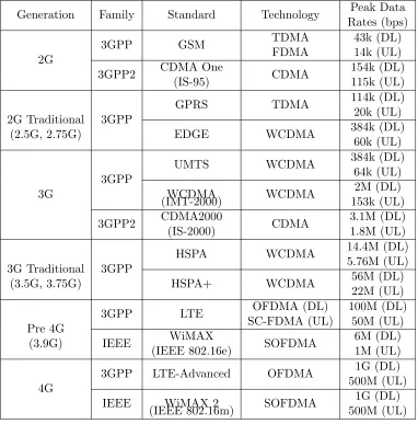
Table 2.1: Evolution of Mobile Telephony Standards and Technologies Generation Family Standard Technology Peak Data

Rates (bps)

2G

3GPP GSM TDMA 43k (DL)

FDMA 14k (UL) 3GPP2 CDMA One CDMA 154k (DL)

(IS-95) 115k (UL)

2G Traditional 3GPP

GPRS TDMA 114k (DL)

(2.5G, 2.75G)

20k (UL)

EDGE WCDMA 384k (DL)

60k (UL)

3G

3GPP

UMTS WCDMA 384k (DL)

64k (UL)

WCDMA WCDMA 2M (DL)

(IMT-2000) 153k (UL)

3GPP2 CDMA2000 CDMA 3.1M (DL)

(IS-2000) 1.8M (UL)

3G Traditional 3GPP

HSPA WCDMA 14.4M (DL)

(3.5G, 3.75G)

5.76M (UL)

HSPA+ WCDMA 56M (DL)

22M (UL)

Pre 4G

3GPP LTE OFDMA (DL) 100M (DL)

(3.9G)

SC-FDMA (UL) 50M (UL)

IEEE WiMAX SOFDMA 6M (DL)

(IEEE 802.16e) 1M (UL)

4G

3GPP LTE-Advanced OFDMA 1G (DL) 500M (UL)

IEEE WiMAX 2 SOFDMA 1G (DL)

(25)

2.2.1 Propagation Mechanisms

The behaviour of radio waves is referred as the radio propagation [2] through wireless

communication channels from transmitter to receiver. Basically, there are three

differ-ent propagation mechanisms which have impact on the radio propagation: reflection, diffraction and scattering. These physical propagation mechanism can be described as

follows:

• Reflection —Radio waves can be reflected back off the surfaces of objects with dimensions which are large in comparison to radio wavelength, for example, the

surfaces of buildings and the earth. The amount of reflection depends on incident

angle, materials and so on.

• Diffraction —Radio waves are propagated around the sharp edge of surfaces, for example, street corners.

• Scattering —Radio waves travel through multiple objects with smaller dimensions compared to their wavelength, for example, rain drops and lamp posts.

2.2.2 Additive White Gaussian Noise Channel

The propagation effects and other signal impairments are often collected and

categor-ically referred to as the channel. The wireless communication channels suffers from a variety of impairments that contribute to errors. Noise, a critical component in the

analysis of the performance of communication systems, are the unwanted signals that affect the fidelity of the desired signal. In wireless communication systems, there are

numerous of noise: thermal noise that exists in all matter, artificial noise from other

electrical machinery and impulse noise from radiation emitting devices [24]. The Ad-ditive white Gaussian noise (AWGN) channel often provides a reasonably good model

in the situation of direct line-of-sight path between transmitter and receiver. The

zero-mean noise having a Gaussian distribution is added to the signal. The noise is always assumed to be white which means that all frequency components appear with equal

power. This channel model can be mathematically described by

(26)

Table 2.2: Path Loss Exponent Values in Different Environments Environment Path Loss Exponent τ

In building line-of-sight 1.6 to 1.8

Free space 2

Obstructed in factories 2 to 3 Urban area cellular 2.7 to 3.5 Shadowed urban cellular 3 to 5

Obstructed in building 4 to 6

wheres(t) is the transmitted time domain signal;n(t) is a sample waveform of a

zero-mean white Gaussian noise process with power spectral density ofN0/2; andr(t) is the

received waveform. There are a great number of ways to combat AWGN, the easiest

one of them is making the transmitting power much higher than that of the noise.

2.2.3 Large Scale Propagation

Based on the general 3-level model of mobile radio propagation, Path loss and Shad-owing are the main cause of large-scale fading in wireless communication. The exact

propagation characteristic is hard to obtain and depends highly on the location,

envi-ronment, etc. The large-scale fading is multiplicative, not additive which is like AWGN [1, 2, 8]. Path loss model is applied for system planning, cell coverage and link

bud-get. Shadowing is employed for power control design and second order interference and

transmit power analysis.

Path Loss

Path loss is caused by the distance between the transmit-receive antennas and the

loss that is due to obstacles and blockages. It leads to steady decreases in the long-term average of signal power as a function of the distance between the transmit-receive

antennas. Denoting a transmitter of power as Pt Watts. When the transmit antenna gain isGtand the receive antenna gain isGr, the received powerPr(d) can be described

as a function ofd[1]

Pr=

PtGtGrλ2

(4π)2_dτ_L (2.2)

whereλis the wavelength of the operation frequency,dis the T-R separation distance

(27)

L= 1 indicates no loss in the system hardware. The path los exponentτ can vary from

1.6 to 6 according to various propagation environments, which can be shown in Table 2.2 [2]. Generally, the value of τ increases with the number of obstructions. τ = 2

corresponds to the line-of-sight (LOS) free space path loss.

The path loss is defined as the difference between the received signal power and the effective transmitted power. It regards signal attenuation as a positive measurement in

dB. For the free space model, the path loss, while antenna gains are included, can be expressed as [2]

P L(dB) = 10 logPt

Pr

=−10 log

GtGrλ2 (4π)2_dτ_L

. (2.3)

It can be seen from (2.3) that pass loss can be also written as

P L(dB) =C+ 10nlogd, (2.4)

with C = 10 log

(4π)2L GtGrλ2

. P L(dB) is a major component in the analysis and

plan-ning of a wireless communication system. In order to compensate for the effect of

path loss, the transmitting power of the signal is increased, within acceptable bounds. Unfortunately, this will not always solve the shadowing problem, because shadowing is

randomly existing.

Shadowing

Shadowing is caused by the changes of radio propagation in the terrain or obstacles, for instances, rural areas with large open spaces, urban areas with tall buildings and

suburban areas with low rises. This effect leads to variation in the short-term average

of signal power or shadow fading. A signal might undergo multiple reflections, which will encounter different power attenuations. Normally, shadowing is associated with

the long-normal distribution [1, 2]. Incorporating the effect of free space path loss, the long-normal shadowing modelP L(d) at a distancedcan be expressed as [2]

P L(d) =P LF(d0) + 10nlog(

d d0

) +Xσ, (2.5)

whered0is a reference distance, andXσ represents the shadowing factor with Gaussian random variables of a zero mean and a standard deviation ofσ, where the value ofXσ

(28)

2.2.4 Small Scale Propagation

Small scale fading, mostly simplified by fading, is referred as the rapid fluctuation of

the multipath delays, amplitudes or phases of a wireless signal over travel distance

or a short period of time, where the large scale path loss effects can be ignored. In small scale propagation, such as multipath, the transmitted signal may arrive at the

receiver with slightly delays. These delays can lead to fluctuations which are caused by the interference between those different versions of transmitted signals [1, 2, 8].

Fading is common in urban areas where transmitters and receivers are surrounded by

structures, trees, moving vehicles and pedestrians, which lead to reflection, diffraction and scattering of the transmitted signals. Unlike large scale pass loss, the effects of small

scale fading are realised over very small distances (a few wavelengths) and are time

dependent. Therefore, the signal with their unique waveforms generated by different paths have randomly distributed amplitudes, phases and delays. The receiver combines

all of these waveforms, which causes the signal distortion and fading.

Root Mean Square Delay Spread

A number of the same copies of the transmitted signal travel through various paths,

and received at different arrivals of times. Some paths give rise to a loss of signal power, while some paths with less obstacles have larger signal power. The span of path

delay in time domain is referred to as delay spread. Generally, a number of multipath

channel parameters are obtained from the power delay profile (PDP), such as mean excess delay, root mean square (RMS) delay spread and excess delay spread. The mean

excess delay ¯τ is the first moment of the PDP, which can be defined as [2]

¯

τ = P

iα2iτi P

iα2i

, (2.6)

where αi and τi denote the path gain and delay for the i-th path, respectively. The

RMS delay spread is the square root of the second central moment of the PDP and can be expressed as

σ = q

¯

(29)

where the second central moment of the PDP can be defined as

¯

τ2₌

P iα2iτi2 P

iα2i

. (2.8)

These delays are measured relative to the first detectable signal arriving at the

receiver at τ0 = 0. If there is only one path i= 1, the RMS delay spread is equal to

zero. The normalised mean excess delay and the RMS delay spread are obtained from

a single PDP. This single PDP is the spatial average of consecutive impulse response

measurements which are averaged and collected through a local area.

Coherence Bandwidth

In general, the coherence bandwidth, denoted as Bc, can be considered as a relation

derived from the RMS delay spread [2]. More simply, it can be regarded as inversely proportional to the RMS delay spread. It is a statistical measure of the range of

frequencies over which the channel can be considered “flat”, that means a channel

passing all spectral components with approximately equal gain and linear phase. In other words, coherence bandwidth is the range of frequencies over which two frequency

components have a strong potential for amplitude correlation. The relation between the coherence bandwidth and the RMS delay spread varies with its definition. In the

case where the frequency correlation function of the bandwidth is 0.5 or above [2], the

coherence bandwidth can be approximately expressed as

Bc≈ 1

5σ. (2.9)

It is obvious that coherence bandwidth is totally depending on the RMS delay spread. The increasing of RMS delay spread leads to decreasing of the coherence

bandwidth. A channel with a large RMS delay spread is highly frequency dispersive.

Doppler Spread

Doppler spread [1], denoted asBd, can be defined as a range of frequencies. In other words, Doppler spread is the measurement of spectral broadening caused by time

(30)

Doppler spectrum is essentially non zero. Between the transmitter and receiver

an-tennas, relative movements of mobiles or objects causes Doppler spread. The Doppler shift fd, or named Doppler frequency, is given by [2]

fd=

ν

λcosθ= ν

cfccosθ, (2.10)

where ν is the relative velocity between transmitter and receiver or other movement

of objectives between them, λ is the wavelength of the carrier frequency and θ is the angle between the direction of the received signal wave and the direction of the mobile

user’s motion. fmax= _λν is defined as the maximum Doppler shift while the angle θis zero. Doppler spreadBdof a channel is equal to the maximum Doppler shift.

Coherence Time

Coherence time, denoted as Tc [2], is the time duration that the fading parameters,

such as channel impulse response, remain fairly constant. In other words, two received

signal sequences have a strong correlation in amplitude within a time duration which can be named as coherence time. In general, coherence time is usually employed in the

time domain to characterise the nature of time varying for the frequency dispersiveness of the channel. If the time correlation function is above 0.5, based on the Clarke’s

Model, the coherence timeTc is given by [9]

Tc≈ 9 16πfmax

, (2.11)

wherefmax is the maximum Doppler shift. Sometimes the Doppler spread and coher-ence time are inversely proportional to one another. That is given by

Tc≈ 1

fmax

. (2.12)

A popular rule of thumb for modern digital communications is to define the coher-ence time as the geometric mean of Equation (2.11) and (2.12), which can be defined

as [2, 24, 9]

Tc= s

9 16πf2

max

= 0.423

fmax

. (2.13)

The definition of coherence time implies that two signals arriving with a time

(31)

Types of Fading

Based on the characteristics of the transmitted signal (such as bandwidth, symbol

period) and the parameters of multipath channel (such as Doppler spread and RMS

delay spread), four types of fading effects are given to describe the fading features [2], which are flat fading and frequency selective fading caused by multipath delay

spread, and fast fading and slow fading due to Doppler spread. These fading effects and conditions are shown in Table 2.3.

• Flat Fading

The channel is regarded as flat fading [1] if the signal bandwidth Bs is much smaller than the channel coherence bandwidthBcand the symbol duration Ts is

much greater than the RMS delay spreadσ. The mobile radio channel will have

constant gain and linear phase response over the transmission bandwidth. In flat fading, the transmitted signal spectral features are preserved at the receiver

side, and so as the multipath structure of the channel. However, the features

of the received signal changes with time according to different distributions such as Rayleigh fading, Rician fading and Nakagami fading [2]. Furthermore, from

Equation (2.9), the coherence bandwidth will be infinite while the RMS delay spread is zero, meaning the channel is frequency flat over all ranges of frequencies.

• Frequency Selective Fading

The channel is regarded as frequency selective fading [1] if the signal bandwidth

Bs is greater than the channel coherence bandwidthBcand the symbol duration

Ts is smaller than the RMS delay spread σ. Under this circumstance in the time

domain, the received signal is distorted, since the received signal is a mixture of multiple versions of the transmitted signals with fading and time delay. Within

the channel, time dispersion of the transmitted waveforms results in frequency

selective fading. Therefore, the overlapped received signals lead to inter-symbol interference (ISI) [2]. In the received signal spectrum, certain frequency

(32)

Table 2.3: Fading Types

Flat Fading Signal Bandwidth<Coherence Bandwidth Frequency Selective Fading Signal Bandwidth>Coherence Bandwidth

Fast Fading Coherence Time <Symbol Duration Slow Fading Coherence Time Symbol Duration

• Fast Fading

The channel is regarded as fast fading if the signal symbol durationTs is larger than the channel coherence timeTc and the signal bandwidth Bs is smaller than

the Doppler spread Bd. Which is to say, the channel impulse response changes rapidly within the symbol duration. This leads to frequency dispersion (or time

selective fading) due to Doppler spread, which causes signal distortion. According

to Equation (2.10) and (2.11), in frequency domain, the signal distortion due to fast fading increases with increasing the mobile speed, because the coherence time

decreases with an increase in Doppler spread.

• Slow Fading

The channel is regarded as slow fading if the signal symbol durationTs is much

smaller than the channel coherence timeTcand the signal bandwidthBsis much

greater than the Doppler spread Bd. In this case, the channel may be assumed to be static over one or several continuous symbol periods.

Flat and frequency selective fading determine the frequency diversity of the

chan-nel while the fast and slow fading determine the time diversity of the chanchan-nel. It is

not specifying that in the nature of the channel is frequency selective or flat fading while a channel is specified as a slow fading or a fast fading channel. Fast fading is

only employed while dealing with the variation rate of the channel due to mobility. For flat fading channels, it can be approximated that there is no time delay in the

impulse response. Figure 2.1 summarised the relationship between the types of fading

(33)

[image:33.612.187.456.79.351.2]

Figure 2.1: Fading channel types

Channel Models

The small-scale multipath channel model is introduced here. It is assumed that each symbol is transmitted through signal bandwidth Bs during symbol period Ts.

Sup-posing the number of the multipath between transmitter and receiver isLch, the time

domain channel impulse response (CIR) h(t) can be given as [2]

h(t) = Lch−1

X

i=0

αiδ(t−τi), (2.14)

where αi and τi are the path gain and delay for theith path, respectively. Note that

the channel reduces to flat fading whenLch= 1.

Assuming that with different delay and different spatial diversity branches are in-dependent,αi is an independent zero mean complex Gaussian random variable, with a

variance following the discrete exponential power delay profile:

E|αi|2 =d·e−

τi

σ, (2.15)

(34)

0 100 200 300 400 500 −35

−30 −25 −20 −15 −10 −5 0 5 10

Time (ms)

Channel Amplitude (dB)

Figure 2.2: A typical Rayleigh fading channel impulse response

In mobile radio channels, the channels distortion [1, 2] can be modelled as a sequence

of complex numbers in the baseband by projecting the RF channel impulse response onto the signal space in two-dimension. The real and imaginary parts of the response

are usually modelled by independent and identically distributed zero-mean Gaussian

random processes. The envelop amplitude of the complex channel response follows the Rayleigh distribution, and its phase follows the uniform distribution. In another words,

each path gain is a complex random variable, of which both real part and imaginary part of the path gain are independent zero mean Gaussian with varianceσ2

r. A typical Rayleigh fading channel impulse response is illustrated in Figure 2.2. The Rayleigh

distribution has a probability density function (PDF) which can be expressed as

P(|αi|) =

|αi|

η2 e

−|αi|

2

2η2 ₀_{≤ |}_α

i| ≤ ∞, (2.16) whereη is the RMS value of the received voltage signal before evelope detection, and

η2 _{is the time-average power of the received signal before envelope detection.}

Clark’s channel model [1, 2, 24], confirmed by measurement in urban area, has been

(35)

2.3 OFDM Systems

For multi-carrier modulation [1, 2], the basic concept is dividing the serial bit stream

into a lot of different parallel sub-streams while transmitting them through the parallel sub-channels. Under ideal cases of the propagation conditions, the sub-channels are

orthogonal to each other in typical. Each sub-channel has a data rate which is much less than that of the total data rate. Consequently, the bandwidth of the corresponding

sub-channel is much less than the whole system bandwidth. In order to make sure

that each sub-channel has a bandwidth which is less than the coherence bandwidth, the number of sub-streams is carefully chosen, by which each sub-channel experiences

relatively flat fading. Therefore, the inter-symbol interference (ISI) on each sub-channel

is small.

2.3.1 OFDM Technology

A high efficient and promising technology, named orthogonal frequency division mul-tiplexing (OFDM) [2], is proposed to combat frequency selective fading channels. By

employing cyclic prefix, the ISI can be completely eliminated. OFDM [25, 26] is one of the effective solutions to frequency selective fading. Compared to previous techniques,

OFDM requires less complex equalisation filters. It has been selected as one of the key

techniques for wireless local area networks IEEE 802.11 standards [27], and has been adopted by LTE-A [5, 28]. Also, it has been chosen as a strong candidate for the WiGig

[29] and the Fifth Generation (5G) wireless communication standards [30, 31] in the

future.

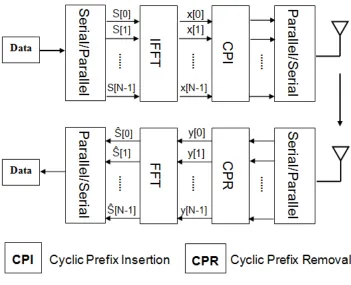
In Figure 2.3, the OFDM implementation of multi-carrier modulation is

demon-strated. The input data stream is modulated by a PSK modulator, resulting in a complex stream with N OFDM symbols as {S[0], S[1], ..., S[N−1]}. Then the sym-bols are converted into time samples by performing an inverse Discrete Fourier

(36)

[image:36.612.143.494.78.363.2]

Figure 2.3: Wireless OFDM system model block diagram

of lengthN can be presented as

x[n] = N−1

X

m=0

S[m]ej2πnm/N, 0≤n≤N−1. (2.17)

Then the cyclic prefix is prepended to each OFDM symbol. Accordingly, the se-quences are ordered with passing through parallel-to-serial converter.

It can be considered that the transmitted waveform passes through the filter of

channel impulse response [2], and then added with the noise (AWGN), which lead to the received signal in time domain. The received signal is then down-converted to

baseband, by which the high-frequency components can be filtered out. After serial-to-parallel convert and CP removal, the received signal sequences y[n] can be given

as

y[n] = L−1

X

l=0

h[l]∗x[n−l] +z[n] 0≤n≤N−1, (2.18) whereh[n] andz[n] are the discrete-time equivalent lowpass CIR and AWGN, respec-tively. These time domain samples are serial-to-parallel converted and passed through

(37)

symbols, whereHnand Z[n] are the CIR and noise associated with then-th

subchan-nel in frequency domain. The DFT output is parallel-to-serial converted and passed through PSK demodulator to recover the original data.

ˆ

S[m] = N−1

X

n=0

y[n]e−j2πnm/N 0≤n≤N −1

=HmS[m] +Z[m]. (2.19)

It can be derived from (2.17) that each transmission data sequence consists of information fromN symbols, and the information of one symbol has been spread across

N transmission data. Therefore, the symbol period in OFDM systems becomes N Ts,

leading to a mitigated ISI. In the frequency domain, the frequency range for each symbol is narrowed toBs/N so that each transmission data carried on one subcarrier

undergoes flat fading.

There are several benefits while utilizing OFDM technique in wireless

communica-tion. First of all, in OFDM systems, each subcarrier suffers from flat fading so the ISI

effect in multipath phenomenon can be eliminated. Secondly, each subcarrier has a nar-row bandwidth, which means that not all of the subcarriers suffer fading in a multipath

channel. Thirdly, each subcarrier can be modulated independently in OFDM systems,

which achieving a higher spectral efficiency than conventional single-carrier systems un-der frequency selective fading channel. Furthermore, OFDM leads to a higher efficiency

in spectrum than the conventional frequency division multiplexing (FDM), where the frequency bands are not overlapped, and there is a guard band between two adjacent

carriers. In OFDM systems, all the subcarriers are orthogonal overlapped, in which

one subcarrier achieves its peak attenuation when others are zeros. This is because of the function of IFFT. Therefore, OFDM system can obtain a higher spectral efficiency

than FDM systems due to the removal of the guard bands.

Therefore, the frequency selective fading channel can be divided into a number of frequency flat fading channels. Thanks to the CP insertion, the ISI can be avoided.

(38)

2.3.2 MIMO OFDM Systems

In order to improve the system capacity, multiple transmit and receive antennas are

employed to establish multiple spatial branches, referred to as MIMO systems [35].

Compared to the traditional SISO systems, MIMO systems can enhance bandwidth efficiency, as multiple transmit and receive antennas operate on the same frequency

band for the signal transmission. OFDM is well suited and employed in MIMO systems to combat the frequency selective fading. Also, equalisation can be simplified in the

frequency domain for OFDM based systems. Therefore, MIMO OFDM systems have

been adopted by the wireless local area network standards (IEEE 802.11) [27] and LTE Advanced, respectively [27, 36, 37].

A MIMO OFDM system is always considered with K transmit and M receive

antennas in the frequency selective fading environment. The incoming serial data at the transmitter is divided into parallel first. Then the IDFT/DFT pair enables the

signal to be transferred in between the frequency domain and the time domain. Let

sk(n, i) denote the symbol on the n-th subcarrier (0 ≤n ≤ N −1) in the i-th block (0≤ i ≤P −1) transmitted by the k-th transmit antenna (0 ≤k ≤ K−1). Define

sk(i) = [sk(0, i), sk(1, i), ..., sk(P−1, i)]T as the signal vector in the i-th block for the

k-th transmit antenna.

At the transmitter, the signal in the i-th OFDM block is first transformed to the

time domain as ˜sk(i) by IDFT as

˜

sk(i) =FHsk(i), (2.20)

where F is an N ×N DFT matrix, with the entry given by F(a, b) = √1 Ne

−j2πab/N_,

(a, b= 0, ..., N −1), and FH is an IDFT matrix, withFH =F−1 since Fis a unitary matrix [38]. The computationally efficient IFFT/FFT pair may also be employed.

The total number of channel path is assumed as L, a CP of length LCP, at least

LCP ≥L−1, is prepended to each OFDM block ˜sk(i). The guard symbols consist of a copy of the lastLCP entries of each OFDM block. The insertion of a CP is aimed to avoid IBI and circular convolution between time-domain signal and CIR. With the CP

(39)

The signal is then transmitted through the frequency selective fading channel, which

is assumed to be constant for the duration of a frame which consists of a total number of P OFDM blocks. This is a convolution process in time domain. The received

signal vector ¯y_m(i) = [¯ym(0, i),y¯m(1, i), ...,y¯m(N −1, i)]T at the m-th receive antenna (0≤m≤M −1) in the time domain can be given as

¯

y_m(i) = K−1

X

k=0

¯

Hm,k¯sk(i) + ¯zm(i), (2.21)

where ¯Hm,kis the convolution chanel matrix with size of (LCP+N)×(LCP+N) between them-th receive antenna and the k-th transmit antenna, which can be expressed as

¯

Hm,k =          

hm,k(0) 0 · · · 0 ..

. hm,k(0) 0 · · · 0

hm,k(L−1) . .. ... ..

. . .. . .. 0

0 · · · hm,k(L−1) · · · hm,k(0)           , (2.22)

wherehm,k(l) is thel-th (0≤l≤L−1) channel path between them-th receive antenna and thek-th transmit antenna, and ¯zm(i) is the AWGN vector whose entries are i.i.d.

complex Gaussian random variable with a zero mean and variance ofN0 [35].

After the CP removal, the received signal can be written as ˜y_m(i) which then is transformed to the frequency domain by applying the N×N DFT matrix as

y_m(i) =F˜y_m(i). (2.23)

The time domain circular convolution can be transformed to a linear

multiplica-tion in the frequency domain by applying the IDFT/DFT operator pair, leading to

simple equalisation for the frequency selective fading environment [39]. The resulting transceiver signal model in the frequency domain can be given as

y_m(i) = K−1

X

k=0

Hm,ksk(i) +zm(i), (2.24)

whereHm,k =FH˜m,kFH is the diagonal frequency domain channel matrix. The entry

(40)

can be preserved by the DFT [35], if the CIR hm,k(l) is assumed to have the Rayleigh

distributed magnitude and uniformly distributed phase. Also, the distribution of the white Gaussian noise samples can be preserved by the DFT.

Finally, the Frequency Domain Equalisation (FDE) can be performed on each

sub-carrier in MIMO OFDM systems, since the frequency selective fading channel is divided into a number of flat fading channels. lets(n, i) = [s0(n, i), s1(n, i), ..., sK−1(n, i),]T

de-note as the signal vector fromK transmit antennas on the n-th subcarrier in the i-th block. The received signal vector y(n, i) = [y0(n, i), y1(n, i), ..., yM−1(n, i),]T in the

frequency domain on then-th subcarrier, which can be given as

y(n, i) =H(n)s(n, i) +z(n), (2.25)

whereH(n) is theM×Kchannel frequency response matrix on then-th subcarrier, with

Hm,k(n) denoting the entry (m, k) in H(n), the channel frequency response between them-th receive antenna and the k-th transmit antenna, and z(n) is the noise vector.

The estimate ˆs(n, i) of the source data can be performed by either Zero Forcing (ZF)

or Minimum Mean Square Error (MMSE) based equalisation on the received signal on then-th subcarrier as

ˆ

s(n, i) =W(n, i)y(n, i), (2.26)

whereW(n, i) is the weighting matrix detected by the ZF or MMSE equalisation cri-terion.

2.3.3 Drawbacks of OFDM Systems

Although OFDM systems can combat frequency selective fading, there are some draw-backs which may degrade the system performance, such as ICI, carrier frequency

off-set (CFO), Inphase/Quadrature (I/Q) imbalance and Peak-to-Average Power Ratio

(PAPR).

ICI

In high mobile fading channel, the time variation of the channel over an OFDM symbol period results in a loss of subchannel orthogonality which leads to ICI [12, 40] due to

(41)

the Doppler spread. The performance degradation becomes significant as the carrier

frequency, block size and vehicle velocity increase [41].

CFO

CFO is another typical radio frequency imperfect [42], and is introduced by frequency

discrepancy between the carrier and the local oscillators. The CFO not only causes interference between frequency bins for frequency domain equalisation, but also

de-grades performance accumulatively with the increase of the block length for block-wise

transmission method [43].

I/Q Imbalance

Due to the drive of low cost and low power consumption, Direct Conversion

Archi-tecture (DCA) has become a trend for the front-end design, particularly in OFDM based wireless communication systems [44]. However, I/Q imbalance is introduced by

the DCA, including frequency independent and frequency dependent I/Q imbalance,

at the transmitter and receiver [45, 46]. Frequency dependent I/Q imbalance is caused by the component mismatching in I and Q branches, and it is frequency selective. On

the other side, frequency independent I/Q imbalance is due to the non-ideal local os-cillators and is constant over the signal bandwidth. I/Q imbalance, if not compensated

for, will introduce an ignorable error floor which can degrade the system performance

severely in MIMO OFDM systems.

PAPR

The transmit signals in an OFDM system can have high peak values in the time domain

since many subcarrier components are added via an IFFT operation. Therefore, OFDM systems are known to have a high PAPR [47], compared with single-carrier systems.

The high PAPR is one of the most detrimental aspects in the OFDM systems, as it

decreases the signal to noise ratio of analogue to digital converter and digital to analogue converter while degrading the efficiency of the power amplifier in the transmitter. the

(42)

2.4 Channel Estimation and Equalisation

After receiving the wireless transmitted signal sequence, the major challenge faced

in OFDM systems is how to obtain the wireless CSI or CIR accurately. With the estimated CIR, a prompt channel equalisation technology can be utilized to recover the

original signal sequence. Channel estimation and equalisation can be classified into the following types: training based, blind or semi-blind based approaches, respectively. For

training based channel estimation and equalisation, a large number of symbol sequences

are needed, while semi-blind or blind approaches require non of the training symbols. Therefore, semi-blind or blind channel estimation and equalisation have higher spectral

efficiency than that of training based approach.

2.4.1 Training Based Channel Estimation and Equalisation

Training Based Channel Estimation

In training based channel estimation approach, the training symbol sequences are known as a priori at the receiver. In order to estimate the source signals, training

symbols are first transmitted for channel estimation. Then, the estimated CSI can be

applied to equalise the source data. This approach is easily applied to any wireless communication systems, and it is the most popular method used today because of its

low computational complexity. However, it has a major drawback that it is wasteful of

the information bandwidth.

Three widely used channel estimation schemes are discussed in this section: least

squares (LS) based channel estimation, minimum mean square error (MMSE) based channel estimation [48, 49] and linear channel interpolation approach [50].

LS based Channel Estimation

The LS based method has been widely applied for wireless channel estimation for its low complexity. Let h = [h0, ..., hL−1, hL, ..., hN−1]T denote the channel vector, of which

elements are assumed to be Gaussian variables and independent to each other. If there

are a total number of L channel paths, then hL = · · · = hN−1 = 0. The channel

response energy is normalised to unity as PN−1

(43)

received signal vector y(i) = [y(0, i), y(1, i), ..., y(N −1, i)]T in the i-th block can be written as

y(i) =X(i)H+z(i), (2.27)

where X(i) = diag{[x(0, i), x(1, i), ..., x(N −1, i)]T} is the N ×N diagonal training matrix, H = √NFh is the channel frequency response vector on N subcarriers, and

z(i) is the noise vector.

Assuming the training blocks is a length with a total number of P, the LS based channel estimation can be performed as

ˆ

HLS = 1

P

P−1

X

i=0

[H+X−1z(i)]. (2.28)

However, the term X−1z(i) may be subject to noise enhancement, especially when the channel is in a deep null.

For MIMO OFDM systems, the channel estimation can be divided into a number of independent SISO OFDM channel estimations, if the training symbols of transmit

an-tennas are orthogonal to each other [51]. It means that a different subset of subcarriers

is applied by each transmit antenna for the training symbols transmission.

MMSE Based Channel Estimation

If the CSI and noise distribution are known, then this priori information can be

ex-ploited to decrease the estimation error for Rayleigh fading channels. This technique usually outperform LS while doing channel estimation, since it can suppress the noise

enhancement for known channel characteristics [52]. The MMSE based channel

esti-mate ˆHM M SEis obtained by minimizing the mean square error, which can be expressed as

minE{kHˆM M SE−Hk2}. (2.29) By substituting the estimated channel vector with LS into Equation (2.29), the

MMSE based channel estimation method can be written as [53]

ˆ

(44)

whereRHH =E{HHH}is the auto-correlation of channel frequency response. MMSE estimation can both decrease the estimation error and shorten the required training sequence. It requires additionally the knowledge of the channel correlation matrix

RHH and noise correlation matrixσz2IN.

Channel Interpolation

Channel interpolation [50] can be employed refine the channel estimation performance

by the LS based technique. The correlation between adjacent subcarriers is used to

correct some incorrect channel estimates for a few subcarriers. By applying the LS based channel estimation as shown in Equation (2.28), ˆHLS can be expressed as in

time-domain channel estimation ˜h as

˜

h= √1

NF

+

N×LHˆLS, (2.31)

where (·)+ denotes the pseudo-inverse, FN×L is the N×LDFT matrix with its entry (a, b) given by FN×L(a, b) = √1_Ne−j2πab/N where (0≤a≤N −1; 0≤b≤L−1). The channel information for all subcarriers can be employed so that ˜h is not influenced by

a few errors on some subcarriers.

Training Based Channel Equalisation

With the estimated CSI, channel equalisation is applied to recover the transmitted

signal on each subcarrier in the OFDM wireless communication systems. A number of

equalisation techniques are discussed here in this subsection: zero forcing (ZF), MMSE and maximum likelihood (ML) based channel equalisation approaches.

ZF based Channel Equalisation

In order to avoid the issues of ISI in OFDM wireless communication systems, the ZF based equalisation method employs the inverse of the channel frequency response to the

received signal in the frequency domain. This technique has been widely used in wireless communication systems since its simplicity. However, it may lead to considerable noise

power enhancement after the process especially when the subcarriers are in deep fading.

(45)

According to the Equation (2.26), the ZF based equalisation method can be performed

on the n-th subcarrier as

ˆ

s(n, i) =WZF(n)y(n), (2.32)

where WZF(n) is the ZF equaliser weight on the n-th subcarrier, which can be given by

WZF(n) = [H(n)HH(n)]−1HH(n). (2.33)

MMSE based Channel Equalisation

The MMSE channel equalisation technique minimises the expected MSE between the

symbol detected at the equaliser output and the transmitted symbols, thereby provid-ing an optimised balance between noise enhancement and ISI mitigation. Since this

balance is favourable in equalisation technology, MMSE equalisers tend to obtain better

BER performance than those equalisers utilising the ZF algorithm. The MMSE based equalisation method is to optimise the MSE as

WM M SE(n) = arg minE{kˆs(n, i)−s(n, i)k2}. (2.34)

Then the MMSE equalisation weight can be obtained by minimising the Equation

(2.34) as

WM M SE(n) =HH(n)[H(n)HH(n) +σz2IM]−1. (2.35)

The source data sequences have a unit variance and are spatially uncorrelated as

Rss =E{s(n, i)sH(n, i)}=IM, and the noise is also spatially uncorrelated with vari-anceσ_z2 asRnn=E{z(n, i)zH(n, i)}=σz2IM.

ML based Channel Equalisation

Maximum-likelihood channel equalisation technique [52] avoids the problem of noise

enhancement because it estimates the sequence of possible transmitted symbols. The ML based equalised signal ˆs(n, i) on the n-th subcarrier in the i-th block for OFDM

wireless communication systems can be given as

(46)

wherex(n, i) and ˜s(n, i) are the received signal vector and the trial transmitted signal

vector, respectively,H(n) is the channel frequency response matrix on the n-th subcar-rier. The ML based equalisation method may need a number of searches, which results

in very high complexity.

2.4.2 Semi-Blind and Blind Channel Equalisation

Unlike training based channel equalisation method, only little information is needed

in the semi-blind equalisation, and non CIR information is required by blind scheme. This highly increases the spectral efficiency. Basically, semi-blind or blind equalisation

techniques exploit the statistics or structure of the received signals and channel char-acteristics to recover the transmitted signals [7]. Based on the statistics order of the

scheme, the equalisation method can be defined as second order statistics (SOS) and

high order statistics (HOS).

SOS based Blind Channel Equalisation

The SOS based blind channel equalisation technique is only feasible for non-minimum

phase channels which are linear and time-invariant, by utilising cyclostationary signals with the periodic correlation [17, 47]. Channels that are invariant and causal whose

inverse or transfer function are known as non-minimum phase channels [47]. It can

provide a greater phase response than the minimum phase channels with equivalent magnitude response.

The SOS based channel identification technique was first proposed in [17] for single-input multiple-output (SIMO) systems, where the non-minimum phase channel is

esti-mated from the auto-correlation of the received signal.

A non-redundant linear precoding was first proposed in [54, 55], where the specific precoding structure is explored for semi-blind channel estimation at the receiver. A

general precoding scheme was designed for channel estimation in [56] by exploiting