GPU acceleration of object classification algorithms using NVIDIA CUDA

Rochester Institute of Technology

RIT Scholar Works

Theses Thesis/Dissertation Collections

9-1-2009

GPU acceleration of object classification

algorithms using NVIDIA CUDA

Jesse Patrick Harvey

Follow this and additional works at:http://scholarworks.rit.edu/theses

This Thesis is brought to you for free and open access by the Thesis/Dissertation Collections at RIT Scholar Works. It has been accepted for inclusion in Theses by an authorized administrator of RIT Scholar Works. For more information, please [email protected].

Recommended Citation

GPU Acceleration of Object Classification Algorithms Using

NVIDIA CUDA

by

Jesse Patrick Harvey

A Thesis Submitted in Partial Fulfillment of the Requirements for the Degree of Master of Science in Computer Engineering

Supervised by

Dr. Andreas Savakis

Department of Computer Engineering Kate Gleason College of Engineering

Rochester Institute of Technology Rochester, NY

September, 2009

Approved By:

_____________________________________________ ___________ ___

Dr. Andreas Savakis, Professor and Head

Primary Advisor – R.I.T. Dept. of Computer Engineering

_ __ ___________________________________ _________ _____

Dr. Muhammad Shaaban, Associate Professor

Committee Member – R.I.T. Dept. of Computer Engineering

_____________________________________________ ______________

Dr. Roy Melton, Lecturer

Thesis Release Permission Form

Rochester Institute of Technology

Kate Gleason College of Engineering

Title: GPU Acceleration of Object Classification Algorithms Using NVIDIA CUDA

I, Jesse Patrick Harvey, hereby grant permission to the Wallace Memorial Library to reproduce

my thesis in whole or part.

_____________________________, Jesse Patrick Harvey

D

EDICATION

This document is dedicated to the family, friends, faculty and staff who have encouraged and

A

CKNOWLEDGEMENTS

This work would not have been possible without the support, advice and encouragement of my

thesis committee. I would like to express my gratitude to my advisor Dr. Andreas Savakis and

the other members of my committee, Dr. Roy Melton and Dr. Muhammad Shaaban.

I would like to thank the staff of the Computer Engineering department. The office staff was

always helpful with dealing with the technicalities of the thesis process while Mr. Richard

Tolleson and Mr. Charles Gruener made sure I had the necessary resources to complete my

work.

Lastly, I would like to thank the students of the Real Time Vision lab and CUDA club who

Abstract

The field of computer vision has become an important part of today’s society, supporting

crucial applications in the medical, manufacturing, military intelligence and surveillance

domains. Many computer vision tasks can be divided into fundamental steps: image acquisition,

pre-processing, feature extraction, detection or segmentation, and high-level processing. This

work focuses on classification and object detection, specifically k-Nearest Neighbors, Support

Vector Machine classification, and Viola & Jones object detection.

Object detection and classification algorithms are computationally intensive, which

makes it difficult to perform classification tasks in real-time. This thesis aims in overcoming the

processing limitations of the above classification algorithms by offloading computation to the

graphics processing unit (GPU) using NVIDIA’s Compute Unified Device Architecture

(CUDA).

The primary focus of this work is the implementation of the Viola and Jones object

detector in CUDA. A multi-GPU implementation provides a speedup ranging from 1x to 6.5x

over optimized OpenCV code for image sizes of 300 x 300 pixels up to 2900 x 1600 pixels while

having comparable detection results. The second part of this thesis is the implementation of a

multi-GPU multi-class SVM classifier. The classifier had the same accuracy as an identical

implementation using LIBSVM with a speedup ranging from 89x to 263x on the tested datasets.

The final part of this thesis was the extension of a previous CUDA k-Nearest Neighbor

implementation by exploiting additional levels of parallelism. These extensions provided a

speedup of 1.24x and 2.35x over the previous CUDA implementation. As an end result of this

T

C

Chapter 1 – Introduction ... 1

Chapter 2 – Background ... 3

2.1 - k-Nearest Neighbor Classification... 3

2.2 - Support Vector Machines ... 5

2.2.1 - Binary Support Vector Machines ... 5

2.2.2 - Multiclass Support Vector Machines ... 7

2.3 - Viola & Jones Object Detection ... 8

2.3.1 - Cascade of Weak Classifiers ... 8

2.3.2 - Integral Image ... 9

2.4 - Graphics Processing Unit (GPU) ... 10

2.5 GPGPU Programming Frameworks ... 12

2.5.1 – Legacy Environments ... 12

2.5.2 – Sh and Brook for GPUs ... 13

2.5.3 - NVIDIA CUDA ... 13

2.5.4 - ATI Stream ... 14

2.5.5 – OpenCL ... 14

2.6 NVIDIA CUDA ... 14

2.6.1 - CUDA Programming Model ... 15

2.6.3 - Memory Hierarchy ... 17

2.6.4 - Compute Capability ... 20

2.6.5 – Occupancy... 21

2.6.6 - Multiple GPUs ... 22

2.6.7 – OpenMP ... 22

Chapter 3 – Previous Work ... 24

3.1 – k-Nearest Neighbor Classification ... 24

3.2 – Support Vector Machines ... 25

3.3 – Viola & Jones Object Detector ... 27

Chapter 4 – GPU Implementation... 29

4.1 - Parallel Primitives... 29

4.1.1 – Reduction ... 29

4.1.2 - Scan ... 31

4.1.3 - Stream Compaction ... 32

4.2 – Algorithm Implementations ... 34

4.2.1 – k-Nearest Neighbor Classification ... 34

4.2.1.1 – Classifying a single test point ... 34

4.2.1.2 – Nearest neighbor classifier (k=1) ... 35

4.2.2 – Support Vector Machines ... 36

4.2.3.1 – Training Data ... 39

4.2.3.2 – Preprocessing ... 40

4.2.3.3 – Context Creation ... 40

4.2.3.4 – Integral Image ... 41

4.2.3.5 – Lighting Correction ... 43

4.2.3.6 – Tree Evaluation ... 43

4.2.3.7 - Stage Evaluation ... 45

4.2.3.8 – Inter-stage Processing ... 46

4.2.3.9 – Window Skipping ... 47

4.2.3.10 - Feature Scaling ... 47

4.2.3.11 – Function Calls ... 50

Chapter 5 – Results ... 53

5.1 – k-Nearest Neighbor Classification ... 54

5.1.1 – Classifying a single test point ... 54

5.1.2 – Nearest Neighbor Classifier (k=1) ... 56

5.2 – Support Vector Machine ... 57

5.3 – Viola & Jones Object Detector ... 60

5.3.1 – OpenCV Versions ... 60

Chapter 6 – Conclusions and Future work ... 73

L

IST OF

F

IGURES

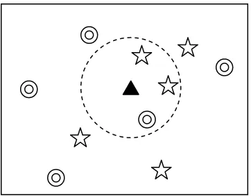
Figure 2.1 – The unknown test point (triangle) is classified as the class that occurs most often

within its closest neighbors. In this case, a star. ... 3

Figure 2.2 -There are many hyperplanes that could be used to separate the two classes of data. .. 6

Figure 2.3 – The optimal hyperplane maximizes the margin or space between the datasets. The points touching the edges of the hyperplane are selected as the support vectors. ... 6

Figure 2.4 - Viola & Jones example face detection cascade ... 8

Figure 2.5 – Feature evaluation using the integral image ... 9

Figure 2.6 - CPU vs. GPU comparison of floating point operations per second. [16] ... 11

Figure 2.7 - CPU vs. GPU bandwidth comparison. [16] ... 11

Figure 2.8 - Transistor allocation for CPU and GPU. [16] ... 12

Figure 2.9 - CUDA Grid layout. [16] ... 15

Figure 2.10 - Common CUDA program flow ... 17

Figure 2.11 - CUDA memory heirarchy. [16] ... 18

Figure 4.1 – Reduction as a tree of operations... 30

Figure 4.2 – Multiple reduction calls to process a list of data ... 31

Figure 4.3 - Binary tree depiction of scan procedure. ... 32

Figure 4.4 - Stream compaction example ... 33

Figure 4.5 - Depection of the 2D reduction. The values down each column are accumulated by the threads in the associated column of the overlapping thread block. ... 36

Figure 4.6 – Multi-GPU multiclass SVM algorithm ... 37

Figure 4.7 - Cascade structure ... 40

Figure 4.9 – Texture fetch conversion from int2 to double ... 42

Figure 4.10 – Tree structure from OpenCV trained classifier data file ... 44

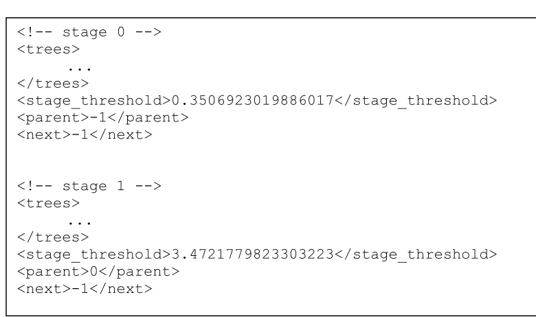
Figure 4.11 – Stage structure from OpenCV trained data file ... 45

Figure 4.12 – Pseudo code for scaled feature weight correction ... 48

Figure 4.13 – Alternating scale iterations are assigned to available GPUs to best balance the workload ... 49

Figure 4.14 - Parallel execution of scale iterations across multiple GPUs ... 50

Figure 4.15 – OpenCV detection function call ... 51

Figure 4.16 – CUDA detection function call ... 51

Figure 5.1 – Results for k-NN single test point classification ... 54

Figure 5.2 – Profiling of the k-NN CUDA implementation for 256 reference points, 1 query point and a dimension of 8192 ... 55

Figure 5.3 - Profiling of the k-NN CUDA implementation for 1024 reference points, 1 query point and a dimension of 8192 ... 56

Figure 5.4 – Results for k-NN nearest neighbor classifier (k=1) ... 56

Figure 5.5 – Profiling of the k-NN CUDA implementation for 8192 reference points, 4 query points and a dimension of 8192 with k=1 ... 57

Figure 5.6 - Profiling of the k-NN CUDA implementation for 8192 reference points, 8192 query points and a dimension of 8192 with k=1 ... 57

Figure 5.7 – Differences between OpenCV versions... 60

Figure 5.9 – CUDA implementation detection results on rehg-thanksgiving-1994, displaying all

detections without grouping ... 61

Figure 5.10 - OpenCV results after averaging and grouping of detected faces ... 62

Figure 5.11 – CUDA implementation results after averaging and grouping of detected faces .... 62

Figure 5.12 – Viola & Jones JUDYBATS results comparison ... 63

Figure 5.13 – Star Trek (original2) classification comparison ... 64

Figure 5.14 – News Radio classification comparison ... 65

Figure 5.15 – Seinfeld classification comparison ... 66

Figure 5.16 – Oksana classification comparison ... 67

Figure 5.17 – Plot of Viola & Jones speedup vs. the number of starting windows in an image .. 69

Figure 5.18 – Plot of speedup with transition to multi-GPU vs. the number of starting windows70 Figure 5.19 – Register usage effect on occupancy ... 71

L

IST OF

T

ABLES

Table 5.1- Number of support vectors in the trained classifiers ... 58

Table 5.2 - Multi-class SVM results for the MNIST database ... 58

Table 5.3 - Multi-class SVM results for the USPS database ... 58

G

LOSSARY

CPU Central Processing Unit

CUDA Compute Unified Device Architecture

CUDPP CUDA Data Parallel Primitives Library

Device A CUDA capable device (GPU)

GPGPU General-purpose computing on graphics processing unit

GPU Graphics Processing Unit

Host Referring to application execution on the CPU

OpenCV Open Computer Vision Library

OpenMP API for multi-platform shared-memory parallel programming

Chapter 1

–

I

The primary focus of this thesis is the efficient implementation of object detection and

classification algorithms on Graphics Processing Units (GPUs). These algorithms are crucial

components of many computer vision algorithms. In order to understand information from an

image or video, objects in the media need to be segmented and classified. It is often desirable to

process these images in real-time, however the object detection and classification algorithms

tend to be very computationally intensive. This work overcomes the processing limitations of the

above classification algorithms by offloading computation to the graphics processing unit (GPU).

The GPU is a massively parallel device which is capable of processing the large amounts

of data required to perform the classification and detection tasks very quickly. Speedups are

obtained over previous implementations by exploiting data independent calculations and

executing them in parallel on the GPU. Two of the algorithms in this work exploit an additional

level of parallelism by running multiple parallel tasks in parallel using multiple GPUs. The

implementations in this thesis were benchmarked against previous works, and the results were

analyzed to explain any performance bottlenecks.

The rest of this thesis is organized in the following manner. Chapter 2 provides the reader

with the background information necessary to understand the implementation details discussed

later. Each algorithm is detailed while the GPU hardware and CUDA are introduced. Chapter 3

describes supporting work for the algorithms covered in this thesis. Additionally, the differences

between the previous work and the current implementations are covered. Chapter 4 discusses the

CUDA implementation for each of the algorithms covered in this work. The implementation

implementation. Both the classification accuracy and timing benchmarks are provided and

discussed. Chapter 6 details possible extensions to the algorithms covered in this work. Lastly,

Chapter 7 provides final conclusions and closing remarks.

Chapter 2

–

B

2.1

-

-N

N

C

K-Nearest Neighbor (k-NN) classification is among the simplest of classification

algorithms and a good first choice when little knowledge about a dataset is available. A query

point is classified by a majority vote of the k closest training points (neighbors), with the object

being assigned to the most common class.

The k-NN algorithm has been used in a wide variety of applications including optical character

recognition [1] [2], content-based image retrieval, signal processing [3] and fraud detection [4].

In the base algorithm, the training phase consists of storing feature vector representations of

training data with associated class labels. Other k-NN algorithms attempt to reduce the number

of distance calculations to be performed. Among these methods are algorithms that organize the

training data into trees [5] or hash the training data into bins [6].

During classification, the query point is represented as a vector in the feature space.

Distances from the query vector to all training vectors are computed, and the k closest samples Figure 2.1 – The unknown test point (triangle) is classified as the class that occurs most often within its closest neighbors. In this

are used to determine the class of the test point. This distance is often the sum of differences

between each element of two data vectors. As an example, the Euclidean distance is provided:

. ) ( 1 2 ) , (



Euclidean p q

D

Several different cases of the k-NN classifier were examined for possible implementation as each

one provides different levels of parallelism.

 Classifying a single test point:

It is often the case that only a single point needs to be classified at a time. Consider for

example, processing a video feed where only a single frame of data is available. In this

case, there are two possible levels of parallelism:

1. Distance calculation between the test point and each training point

2. Difference calculations for the distance calculation between the test point and

each training point

As it offers a finer grain of parallelism, the latter case provides a greater number of

independent calculations for the GPU to process. As reported in Section 5.1.1, exploiting

these extra calculations provides a speedup over an existing CUDA k-NN

implementation.

 Classifying multiple test points at a time:

Having multiple test points available for classification provides much more data for the

GPU to process. In this case, the distances between all test points and support vectors can

k distances. This case provides the greatest level of parallelism and a sufficient amount of

computation to utilize the GPU fully and efficiently.

 Nearest neighbor classifier (k=1):

If only the nearest neighbor is used to classify the test point, a different approach can be

used for the final classification. When k is greater than one, the k shortest distances must

be determined, often with a sort. As reported in Section 5.1.2, when only the single

shortest distance is required, finding the minimum value can be less costly than

performing a full sort.

2.2

-

S

V

M

Support Vector Machines (SVMs) [7] are another method for classifying data. This is

done by constructing a hyperplane that separates the classes. The base SVM implementation is a

binary classifier, which is only able to differentiate between two classes. SVMs have also been

adopted to solve multiclass problems [8] [9]. SVMs have been used for many applications

including face detection [10], data mining [11] and medical diagnosis [12].

2.2.1 -BINARY SUPPORT VECTOR MACHINES

The base SVM is a binary classifier. Binary support vector machines are able to differentiate

only between two classes. During the training phase, a hyperplane is found that separates the two

different classes with a maximum margin as seen in Figure 2.3 below. Only the training points

During classification, the algorithm merely needs to determine on which side of the

hyperplane the query point lays. This can be done by computing a relatively simple decision

function:

𝐼 𝑧 = 𝑠𝑖𝑔𝑛 𝛼𝑖𝐾 𝑧, 𝑐𝑖 + 𝑏0 𝑆𝑢𝑝𝑝𝑜𝑟𝑡𝑉𝑒𝑐𝑡𝑜𝑟𝑠

α = Support vector weight c = Support vector z = Test vector b = bias

K = kernel function

The kernel function above should not be confused with CUDA terminology. The SVM

kernel is a function that maps the input data into a higher dimensional space so the two classes

can be separated more easily. Common kernels include:

 Linear: 𝐾_{𝐿𝑖𝑛𝑒𝑎𝑟}(𝑎, 𝑏) = 𝑎 ∙ 𝑏𝑇

 Polynomial of degree n: 𝐾_{𝑃𝑜𝑙𝑦𝑛𝑜𝑚𝑖𝑎𝑙} 𝑎, 𝑏 = (𝑎 ∙ 𝑏𝑇_{+ 1)}𝑛

 Radial Basis Function (RBF): 𝐾_𝑅𝐵𝐹 𝑎, 𝑏 =− 𝑎−𝑏 _2𝜎2 2

Figure 2.3 – The optimal hyperplane maximizes the margin or space between the datasets. The points touching the edges of the hyperplane are selected as

the support vectors. Figure 2.2 -There are many hyperplanes that could be

2.2.2 -MULTICLASS SUPPORT VECTOR MACHINES

The multiclass support vector machine extends the functionality of the binary support vector

machine to enable classification between three or more classes. The primary algorithms for

multiclass SVMs split the classification problem into multiple binary problems, each with its

own classifier. The two dominating implementations are:

 One-against-all classification:

The one-against-all (OAA) classifier requires a trained SVM for each class. During

training, the label for the targeted class is set to positive while all other labels are set

to negative. During classification, each test point is run through each of the

classifiers. The test point is then assigned to the class with the maximum classifier

response.

 One-against-one classification:

In the one-against-one (OAO) algorithm, a SVM is trained to differentiate between

each possible pair of classes. During classification, each test point is run through all

classifiers, and the point is assigned to the class chosen by the greatest number of

classifiers.

The accuracy of these classifiers was compared in [13]. The error rates were similar for

both algorithms across the datasets studied. From the aspect of this work, the classification

process for each is similar:

 Run each test point through each of the trained classifiers

As such, the one-against-all classifier was selected for implementation but the one-against-one

classifier would have been an equally plausible choice.

2.3

-

V

&

J

O

D

Viola & Jones [14] is a commonly used object detection algorithm that is well-known for

its face detection performance.

2.3.1 -CASCADE OF WEAK CLASSIFIERS

The Viola and Jones object detector is a strong classifier composed of many weak

classifiers. These weak classifiers are simple to allow for fast processing, only performing a

weighted sum of rectangular features. By combining these weak classifiers into a cascade, a final

classifier is created that is able to eliminate non-face regions quickly while keeping nearly all

face regions.

In order to process images in real-time, the earlier cascade stages have a limited number

of features and attempt to remove only windows that have a low probability of being faces. As

the cascade stages progress, a greater number of increasingly complex classifiers are used to

Stage 0: 3 features

NOT

Face Face

Stage 1: 9 features

Stage 19: 108 features

Not Face Not Face Not Face

Face Face

Face …

reduce false positive classifications. If one of the cascade stages classifies a window as non-face,

no further stages process it. This ensures that only the regions with a high probability of being

faces will be subjected to the more intensive computations.

2.3.2 -INTEGRAL IMAGE

Viola and Jones were the first to introduce the concept of an integral image or summed

area table (SAT). The integral image at location x, y contains the sum of the pixels above and to

the left of x, y, inclusive.

𝑖𝑖 𝑥, 𝑦 = 𝑖(𝑥′, 𝑦′)

𝑥′≤𝑥,𝑦′≤𝑦

Using the integral image, the sum of any rectangular feature can easily be calculated with only a

few array lookups rather than a runtime pixel by pixel summation. A feature at location (x, y)

with width w and height h can be calculated using the integral image with four array references.

) 1 , 1 ( ) 1 , 1 ( ) 1 , 1 ( ) 1 , 1 ( ) , , ,

(x y wh ii x y ii xw yh ii x yh ii xw y RecSum

These lookups are depicted in Figure 2.5 below.

R

R

e

e

c

c

S

S

u

u

m

m

(

(

x

x

,

,

y

y

,

,

w

w

,

,

h

h

)

)

ii(x-1, y-1)

ii(x-1, y+h-1)

ii(x+w-1, y-1)

ii(x+w-1, y+h-1)

A variant of the integral image stores the squared sum for use in calculating the standard

deviation.

𝑖𝑆𝑖 𝑥, 𝑦 = 𝑖 𝑥′, 𝑦′ 2

𝑥′_≤𝑥,𝑦′_≤𝑦

Tilted features are not within the scope of this thesis, however their support would

require an additional integral image. As described in [15], a rotated integral image can be used to

compute the values of 45º rotated rectangles. The rotated integral image is defined as the sum of

the pixels of a rotated rectangle with the bottom most corner at (x, y) and extending upwards to

the boundaries of the image.









'

,'

)

,

(

y

x

i

y

x

iRi

In order to detect objects of different sizes, the classifier is run over the image multiple

times. Before each iteration, the classifier window and features are scaled larger until one of the

window dimensions is greater than its associated image dimension. These independent iterations

provide a source of parallelism, allowing multiple feature scales to be processed in parallel.

In order to find objects at different locations in an image, the classifier window slides

across the image. As the window slides across the image, the step size or spacing between one

window and the next is a function of the current feature scale. Processing independent windows

at multiple locations offers an additional level of parallelism.

2.4

-

G

P

U

(GPU)

Traditionally, graphics processing units have been used as dedicated rendering devices

increasingly programmable and are now capable of performing much more than graphics specific

computations. The specialized rendering hardware provides an advantage for the GPU over the

CPU when performing compute-intensive, highly parallel computations.

Figure 2.6- CPU vs. GPU comparison of floating point operations per second. [16]

This advantage is primarily due to the transistor allocation for the GPU vs. the CPU. The

majority of the transistors on the GPU are devoted to data processing rather than flow control

and data caching.

Figure 2.8- Transistor allocation for CPU and GPU. [16]

2.5

GPGPU

P

F

The GPU is a powerful device, capable of processing a massive amount of data in a short

amount of time. However, software is required to program the GPU actions, and programming

interfaces are required to access the hardware.

2.5.1 –LEGACY ENVIRONMENTS

Early GPGPU relied on lower level languages such as OpenGL for programming the

devices. OpenGL is primarily used for programming 2D and 3D graphic applications but

provides access to the hardware that GPGPU requires. GPGPU programming through OpenGL

requires a great deal of knowledge about the hardware such as textures and shaders.

Programming through OpenGL and other early frameworks is considered a very low level

2.5.2 –SH AND BROOK FOR GPUS

Sh and Brook for GPUs (BrookGPU) were two of the earliest high-level languages and

programming environments. These programming frameworks provide a level of abstraction from

the graphics hardware so the programmer does not require in-depth knowledge of GPU textures

and shaders.

BrookGPU is a compiler and runtime implementation of the Brook stream programming

language, and it is implemented as an extension to the C programming language. Sh is a

metaprogramming language that is implemented as a C++ library. Both BrookGPU and Sh

support NVIDIA and ATI GPUs on both Windows and Linux. Sh has been commercialized and

expanded with additional support for the cell processor and multicore CPUs. BrookGPU has

been adopted for use in ATI Stream.

2.5.3 -NVIDIACUDA

NVIDIA realized the necessity for an easy method to program these powerful devices.

“In November 2006, NVIDIA introduced CUDA, a general purpose parallel computing

architecture – with a new parallel programming model and instruction set architecture – that

leverages the parallel compute engine in NVIDIA GPUs to solve many complex computational

problems in a more efficient way than on a CPU.” [16]

As CUDA is a framework built around the C programming language, CUDA applications

are fairly easy to implement. However, a great deal of time and knowledge is required to

optimize the applications for the specialized hardware. Special care has to be taken with memory

access patterns and algorithm design to obtain maximum efficiency. CUDA is cross-platform but

2.5.4 -ATISTREAM

ATI Stream by AMD is a similar concept to that of NVIDIA’s CUDA. Both provide a

high level interface for programming the stream processors on the GPUs. ATI Stream utilizes

Brook+, a compiler and runtime package for GPGPU programming to provide control over GPU

hardware. ATI Stream is cross-platform but only runs on AMD GPUs. ATI Stream and CUDA

both have their positives and negatives. For the work of this thesis, NVIDIA’s CUDA was

preferred over ATI Stream for its previous use at the institution.

2.5.5 –OPENCL

NVIDIA and AMD both plan to support OpenCL (Open Computing Language). OpenCL

is the first open standard for general-purpose parallel programming of heterogeneous systems.

OpenCL supports not only GPU programming but also a diverse mix of multi-core CPUs, GPUs,

Cell-type architectures and other parallel processors such as DSPs. OpenCL will provide a

programming framework and environment most closely related to NVIDIA’s CUDA. During the

time period of this work, OpenCL was still very new so it was not considered for

implementation. However, it is believed the transition from CUDA to OpenCL would be a

relatively straightforward process.

2.6

NVIDIA

CUDA

As the majority of work required for this thesis is the implementation of existing

sequential algorithms using CUDA, some details regarding CUDA development must first be

2.6.1 -CUDAPROGRAMMING MODEL

CUDA programmers develop code for the GPU by creating C functions called kernels.

Only one kernel can be run on the device at a time, and all configured threads execute the kernel

in parallel. The threads are grouped into thread blocks which are then organized in a grid as seen

in Figure 2.9 below.

When a kernel is launched, the blocks of the grid are distributed to multiprocessors with

available execution capacity. The threads of a block execute concurrently on a single

multiprocessor. As each thread block completes its work, the multiprocessors are freed, and a

new block is launched in its place.

To manage the numerous threads, the multiprocessor employs a single-instruction,

multiple-thread (SIMT) architecture. This allows each thread to execute independent of the other

threads on one of eight scalar processors. Instructions are issued to groups of 32 threads called

warps, which execute one common instruction at a time. If the instructions assigned to threads

within a warp differ due to conditional branching, the warp executes each path sequentially while

disabling threads that are not on the path. When all branch paths are complete, the threads join

back to the common execution path. It is for this reason that code within conditional statements

such as if/else should be limited.

Given the above information, it is now relevant to note that the GPUs of concern for this

work have the following specifications:

 The maximum number of threads per block is 512

 The maximum size of each dimension of a grid of thread blocks is 65535

 The maximum number of active blocks per multiprocessor is 8

 The maximum number of active threads per multiprocessor is 1024

 The maximum number of active warps per multiprocessor is 32

CUDA also provides limited synchronization between threads of the same block via the

syncthreads function call. Upon hitting a syncthread, each thread will wait until all remaining

threads reach the call. Syncthreads is primarily used to coordinate communication between the

threads within a block to prevent read/write data hazards with shared or global memory. The

only way to synchronize across thread blocks is by breaking the computation into multiple

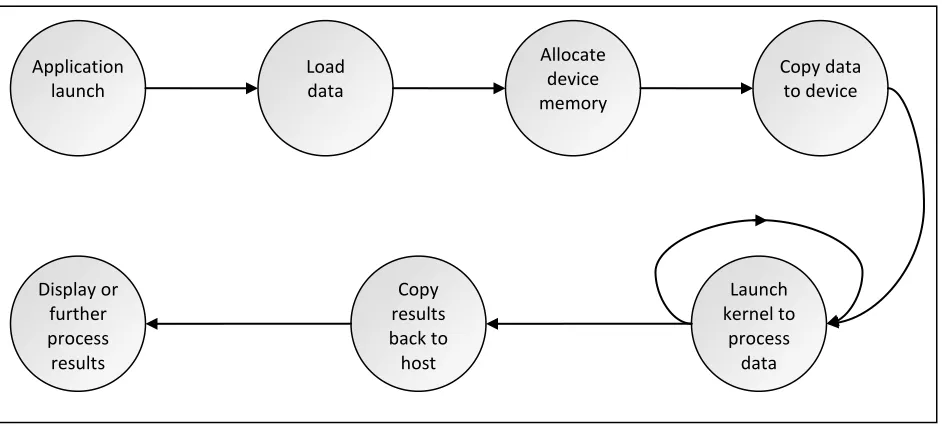
2.6.2 –CUDAPROGRAM FLOW

Most CUDA applications follow a set program flow. The host first loads data from a

source such as a text file and stores it into a data structure in host memory. The host then

allocates device memory for the data and copies the data to the allocated space. Kernels are then

launched to process the data and produce results. These results are then copied back to the host

for display or further processing.

2.6.3 -MEMORY HIERARCHY

As shown in Figure 2.11 below, there are five main regions of memory on the device.

 Device Memory: All threads have read/write access to the device DRAM.

 Registers: Each multiprocessor has read/write access to a limited number of 32 bit hardware

registers.

 Shared Memory: All threads within a block have access to a common shared memory region.

The amount of shared memory available per multiprocessor is limited to 16 KB with a small

quantity reserved for built in variables. Application launch Load data Allocate device memory Copy data to device Launch kernel to process data Copy results back to host Display or further process results

 Constant Memory: A read-only constant cache is shared by all scalar processor cores and

speeds up reads from the constant memory when all threads of a half warp access the same

location. The total amount of constant memory is 64 KB. The cache working set for constant

memory is 8 KB per multiprocessor.

 Texture Memory: A read-only texture cache is shared by all scalar processor cores and

speeds up reads from the texture memory space. The texture cache is optimized for 2D

spatial locality, so threads of the same warp that read texture addresses that are close together

will achieve best performance. The cache working set for texture memory varies between 6

and 8 KB per multiprocessor.

CUDA also has a “local” memory space, which has the same speed as device memory. Local

memory is automatically used to store local scope arrays and additional variables if there are

insufficient registers available. The above mentioned data is summarized in Table 2.1 below.

Table 2.1 - Summary of CUDA memory heiarchy [17]

Memory Location Cached Access Scope

Register On-chip No Read/Write Individual thread Local Off-chip No Read/Write Individual thread

Shared On-chip No Read/Write All threads within a block Global Off-chip No Read/Write All threads + host

Constant Off-chip Yes Read All threads + host Texture Off-chip Yes Read All threads + host

The global memory bandwidth is used most efficiently when simultaneous memory

accesses by threads in a half-warp can be coalesced into a single memory transaction of 32, 64,

or 128 bytes. On devices with compute capability 1.3, coalescing is achieved for any pattern of

addresses requested by the half-warp as soon as the words accessed by all threads lie in the same

segment of size equal to:

 32 bytes if all threads access 8-bit words,

 64 bytes if all threads access 16-bit words, and

 128 bytes if all threads access 32-bit or 64-bit words .

If a half-warp addresses words in n different segments, n memory transactions are issued;

therefore it is necessary to arrange data so that they can be read from global memory in a

coalesced manner. If coalescing reads is not possible, use of the texture cache is often the next

While discussing memory, it is worth mentioning zero copy. Introduced in CUDA 2.2,

zero copy allows GPU threads to access host memory directly. When data are written to zero

copy allocated memory from the device, the data transfer is automatically overlapped with kernel

execution. This however requires the host to synchronize explicitly with the device before

attempting to read any zero copy memory. Zero copy requires that the device can map host

memory; this can be checked by calling cudaGetDeviceProperties() and checking the

canMapHostMemory property.

2.6.4 -COMPUTE CAPABILITY

The compute capability of a device is defined by a major revision number and a minor

revision number. Devices with the same major revision number are of the same core architecture.

The minor revision number corresponds to an incremental improvement to the core architecture,

possibly including new features.

The algorithms in this work were developed to utilize the features of newer devices with 1.3

compute compatibility. The main advantages of compute capability 1.3 devices over earlier

devices include:

 Support for double-precision floating point numbers

 16,384 registers per multiprocessor vs. 8,192

 Support for atomic functions operating in shared memory

 Support for atomic functions operating on 64-bit words in global memory

2.6.5 –OCCUPANCY

Occupancy is defined as the ratio of the number of active warps per multiprocessor to the

maximum number of active warps. A higher occupancy results in the hardware being more fully

utilized. The greatest benefit from high occupancy is the latency hiding during global memory

loads. An increase in occupancy does not guarantee higher performance. As discussed in Section

2.6.1, each multiprocessor has a limited set of registers and shared memory. These resources are

shared between all thread blocks running on a multiprocessor.

Occupancy can be increased by decreasing the resources used by each thread in a block,

or by decreasing the number of threads launched in each block. As shared memory is manually

managed, local or global memory can easily be substituted instead. Register usage is more

difficult to manage as registers are automatically used during memory transfers and calculations.

CUDA provides two additional mechanisms to limit register usage.

 The maxrregcount compiler flag can be used to specify the maximum number of

registers each CUDA kernel can use. If specified, the compiler uses local memory rather

than the extra registers.

 The volatile keyword can also be used to limit register usage. Rather than immediately

evaluating a variable, the CUDA compiler may inline it to be evaluated later. This can

result in redundant calculations if the variable is used more than once. Each time the

variable is computed, additional registers may be used, increasing the register count. The

volatile keyword is essentially a method for suggesting that the compiler evaluates the

2.6.6 -MULTIPLE GPUS

CUDA supports the use of multiple GPUs in a single application. The GPUs are

completely independent of each other, with their own memory space and instructions. Each GPU

must be programmed and setup separately. Generally, a CPU thread is launched to manage each

GPU. The OpenMP API was selected to manage the host threads.

2.6.7 –OPENMP

OpenMP is a shared memory multiprocessing API that was selected to manage the host

level parallelism as it is:

 Multi-Platform

 A C/C++ interface

 Portable and Scalable

 Used by OpenCV1

OpenMP uses preprocessor directives to signify parallel blocks of code. For this work, the

typical OpenMP usage includes:

 Set number of OpenMP threads to be equal to the number of GPUs in the system using

omp_set_num_threads()

 Perform serial code block

 Execute parallel code block via preprocessor directive #pragma omp parallel

 Join threads

 Execute serial code block

The next chapter examines some of the previous work that has been done with these

algorithms. Previous implementations and attempts at accelerating the algorithms are introduced

Chapter 3

–

P

W

The algorithms implemented in this thesis have already been functionally proven.

However, the required computation time often makes them impractical for use in real time

computer vision tasks. CUDA has been successfully used to accelerate applications in many

fields including cryptography [18], mathematical model simulations [19] and image processing

[20]. Many applications report speedups in the range of 1.5x to 400x depending on the degree of

parallelism in the algorithm.

3.1

–

-N

N

C

Since the introduction of k-Nearest Neighbors, many attempts have been made to

improve its performance. Many of these optimizations focus on restructuring or reformatting the

data to help minimize the search space for nearest neighbors.

The k-d tree method [5] relies on organizing the data into a binary tree where each

training point is stored as a node. Once established, the k-d tree allows a search to be performed

over only the closest neighbors of a query point, greatly reducing the work that has to be done.

While the use of k-d tree increases performance by decreasing the search space, it relies on

complex data structures and recursive tree traversal algorithms, neither of which map well onto

the GPU.

Gionis et al. [6] note that “if the number of dimensions exceeds 10 to 20, searching in k-d

trees and related structures involves the inspection of a large fraction of the database, thereby

doing no better than brute-force linear search” and instead examine a scheme for approximate

similarity search based on hashing. During training, a method called locality sensitive hashing

query point can then be accomplished by hashing the point and retrieving elements stored in the

bin that would contain the hashed query point.

As with k-d trees, the hashing method requires that the training data be preprocessed in

order to optimize classification. Instead of manipulating the training data for a more efficient

search, this work focuses on a linear search approach of computing the distance to all neighbors.

This approach exploits the parallelism of independent points and the underlying computations to

obtain a speedup over sequential implementations.

The brute force approach has been implemented on CUDA in [21]. This implementation

exploits multiple test points as the main source of parallelism as it computes and sorts distances

in parallel. This thesis extends the work in [21] by adding functionality to exploit different

sources of parallelism when dealing with fewer test points.

3.2

–

S

V

M

The original foundation for Support Vector Machines was introduced in [22]. Since then,

several implementations have followed including LIBSVM and the SVM functionality of

MATLAB’s Bioinformatics Toolbox. Both of these applications provide the ability to train and

classify a support vector system. At the time of writing, LIBSVM [23] supported linear,

polynomial, RBF and sigmoid kernels, while MATLAB supported linear, polynomial, RBF,

multilayer perceptron (MLP) and user generated kernels.

In an effort to exploit the parallelism in SVM classification and training, two parallel

CUDA implementations have been developed. GPUSVM [24] reports a speedup of 81-138x over

CUBLAS2 to perform dot product calculations in parallel followed by a parallel reduction to

compute the classification sum for each test point.

CUSVM [25] followed GPUSVM with a similar implementation that also included

regression and support for mixed precision arithmetic. CUSVM supports only the Gaussian

kernel and few details on the classification implementation are provided. A speedup of 22x -

172x over LIBSVM is reported for various datasets.

In order to handle greater amounts of data and exploit additional parallelism, [26] used

CUDA to implement an incremental least squares SVM (LS-SVM) for handling billions of data

points with high dimensionality (up to 103). A speedup of 65x over a sequential CPU

implementation and over 1000x over LIBSVM is reported. LS-SVM processes chunks of data

points in parallel on the GPU using the vendor supplied CUBLAS library for matrix operations.

The calculation results are copied back to the CPU for final classification.

Zhang et al. [27] also take advantage of multiple test points by using a SVM to classify

windows, or sub-regions of an image in parallel. The GPGPU scan-window based object

detection framework was used to detect pedestrians with a speedup of “more-than-ten-times”

over a sequential CPU implementation. The low level GPGPU implementation process varies

greatly from that of CUDA.

As with k-NN, these previous works target multiple query points as the main source of

parallelism and design the parallel algorithms to exploit it best. This work used a previous SVM

implementation to exploit a different source of parallelism, multiple classifiers running across

multiple GPUs to create a multiclass SVM classifier.

3.3

–

V

&

J

O

D

Viola and Jones introduced their object detection algorithm in [14]. This algorithm is

extended in [15] with the addition of rotated features and alternative boosting algorithms. This

extended algorithm was implemented as part of the OpenCV library. The OpenCV

implementation offers the ability to enable OpenMP to distribute strips of an image across

multiple CPU threads. The use of OpenMP allows OpenCV to exploit parallelism, but not at the

level of GPUs.

The concepts introduced by Viola and Jones are not only applicable for their object

detector. Several phases of the object detection process have been parallelized for use in other

projects. For example, [28] introduces a new integral image algorithm for the GPU. The

algorithm was implemented in Brook and uses parallel prefix sum operations to compute the

integral image in stages. A speedup of 10x over “the best available CPU implementation” was

reported for large images. Allusse et al. [29] also implement parallel integral image generation

but use the CUDPP3 library to perform the parallel sums for a speedup ranging from ~0.06x for

128x128 images to ~3x for 2048x2048 images.

While no other CUDA implementations of the Haar classifier based object detector could

be found, parallel implementations exist for other platforms. The work in [30] processes up to

three feature classifiers in parallel using a FPGA hardware architecture for a 35x speedup over a

similar sequential CPU implementation.

An exceptional amount of knowledge can be gained from the previous work, especially

the OpenCV implementation. However, implementing the Viola & Jones object detector on

CUDA required a substantially different implementation process.

The next chapter discusses this thesis’ GPU implementation of k-Nearest Neighbor

Classification, Multi-class Support Vector Machines and Viola and Jones Object Detection. This

includes both the high level algorithms and data parallel primitives that are required to perform

Chapter 4

–

GPU

I

Many computer vision tasks require fast response times. The proposed algorithms can be

very computationally intensive, making them difficult to use for real-time tasks. By taking

advantage of the parallel nature of these algorithms, execution on the GPU can be done in a

fraction of the original time. Offloading processing to the GPU also frees the CPU for other

tasks such as device IO, reporting or user interaction.

4.1

-

P

P

A set of data-parallel algorithm primitives are used quite frequently to implement parts of

larger algorithms. Fortunately, a variety of these parallel primitives have already been

implemented in CUDA.

 Several of these are implemented as examples in the CUDA Software Development

Kit (SDK).

 The CUDA Data Parallel Primitives (CUDPP) library also provides several

implementations.

 Thrust is an open-source library that provides a high-level interface to many of these

parallel primitives.

Several of these primitives are used as part of the algorithms implemented in this thesis; any

libraries used will be detailed in later sections.

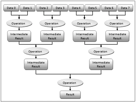
4.1.1 –REDUCTION

A reduction is a method for processing a list of data elements to build up a single return

value. In this thesis, reductions are used to find the sum and minimum value in a list of elements.

The operation for a sum reduction would be addition and min for a minimum reduction.

This process maps well onto the GPU where each thread block is responsible for reducing

a section of the data array. Each block produces a result and all of these results must then be

combined. This is accomplished by calling the kernel an additional time to reduce these results.

Operation

Result Data 0 Data 1

Operation

Intermediate Result

Operation

Intermediate Result

Data 2 Data 3

Operation

Intermediate Result

Data 4 Data 5

Operation

Intermediate Result

Operation

Intermediate Result

Data 6 Data 7

Operation

Intermediate Result

As the operations involved in a reduction tend to be very simple, each thread within a

block does very little work. In order to hide latencies, it is often beneficial to have a single thread

process multiple elements. This is done by having each thread perform the operation while

reading multiple data points from global memory into shared memory. Once the data is in shared

memory, all threads work together to reduce the data. Additional information regarding the

NVIDIA SDK reduction implementation, including code, is available in the NVIDIA whitepaper

[31].

4.1.2 -SCAN

A scan, also known as a prefix sum, is an algorithm that produces an output array in

which every element is the sum of the elements before it. For example, an input of





would produce the array



 

 







Call 0 – 4 blocks

In the CUDA SDK scan implementation, the threads within a thread block work together

to process the data in two phases. The first phase is called the up-sweep or reduce phase. This

phase performs a reduction to compute and store the intermediate partial sums. The second phase

is referred to as the down-sweep phase in which the partial sums are used to populate the output

array. As noted in [32], this process is most easily depicted as a binary tree:

Figure 4.3 - Binary tree depiction of scan procedure.

At each level of the down-sweep phase, each vertex is passed to the left child while the sum of

the vertex and the left child from the up-sweep phase is passed to the right child. The binary tree

data structure does not map well onto the GPU; it is merely a concept used to determine what

elements the threads in a block process. The above figure depicts an exclusive scan, where each

element in the results of a scan contains the sum of all previous elements. An inclusive scan contains

the sum of all elements up to and including the value at the index. The inclusive scan can be

constructed by shifting the results from an exclusive scan left and inserting the total sum in the

last position. Additional information regarding the NVIDIA SDK scan implementation,

including code is available in the NVIDIA whitepaper [33].

4.1.3 -STREAM COMPACTION

The stream compaction algorithm is used to remove unwanted values from an array of

decreasing memory usage, memory transfer bandwidth requirements and wasted processing.

Stream compaction requires two phases, the first of which determines the output indices for the

valid input data. The second phase places the input data into the output array at the indices

generated in the previous phase.

The first phase requires a secondary array that has a value of 1 in indices of important

values and a 0 in the indices of all other values. A scan is then performed on this array to

generate the output indices. This array is used as a lookup table to place the actual input values

into the output array as in the following example:

Stream compaction is implemented with two kernel calls. The first of which processes the scan,

and the second handles the copy to the output.

1 1 0 0 1 0 1 1 0 0 0 1

0 1 2 2 2 3 3 4 5 5 5 5 + + + + + + + + + + + 4 5 -1 -3 8 -2 6 9 -4 -9 -1 1

4 5 8 6 9 1

4 5 -1 -3 8 -2 6 9 -4 -9 -1 1

0 1 2 2 2 3 3 4 5 5 5 5 Phase 1: Scan

Phase 2: Copy to output

4.2

–

A

I

4.2.1 – K-NEAREST NEIGHBOR CLASSIFICATION

The work in [21] already provides a very fast and efficient implementation of the base

k-NN algorithm. The basic algorithm of this work is:

 Compute the distances from all test points to all known vectors in parallel

 Sort the distances for each test point in parallel

 Take the square root of the closest k distances in parallel

 Copy the results from the GPU to the CPU

Rather than duplicating this work, this thesis focused on optimizing the implementation for two

different cases: classifying a single test point and classifying test points when k=1.

4.2.1.1– Classifying a single test point

As the previous work focused on classifying multiple test points at a time, there was

sufficient data to fully and efficiently utilize the GPU without utilizing the finest grain of

parallelism. In the previous implementation, each thread was responsible for computing the

distance from a reference point to a query point by calculating

.

)

(







p

p

q

D

With only a single test point however, additional parallelism must be exploited to utilize

the device fully. The new implementation breaks the distance calculation apart, making each





i

i q

p 

A parallel reduction is then used to accumulate the partial sums for each distance computation.

The previous algorithm resumes with a parallel sort of the distances to find the k closest

neighbors.

4.2.1.2– Nearest neighbor classifier (k=1)

The change to the algorithm in this case is simply substituting the parallel sort with a

minimum reduction. The CUDA SDK reduction example was used as the base reduction

algorithm. However, several changes were necessary.

 The base reduction would simply return the minimum value of the list. For this

implementation, the index of the minimum value is also required. This requirement not

only introduces extra overhead, but also introduces divergent branches into the algorithm.

Fortunately, very limited work is done within the branches so the branch penalty should

be minimal.

 The base reduction is designed to handle one-dimensional data arrays while the k-NN

data is two-dimensional. A naive solution would be to call the reduction kernel once for

each column of data. However, this will result in a great deal of kernel launch overhead.

Another approach would be to launch a thread block to reduce each column of the array.

This approach is more efficient than the previous but is still not optimal. The limited

number of threads per block makes it impossible to control how many values each thread

is responsible for accumulating before the reduction. Instead, a reduction was

implemented which used two-dimensional thread blocks. The threads in a column work

this manner, the threads within multiple blocks work together to reduce multiple columns

of the array at a time.

The initial reduction results in multiple partial sums for each column. These values are

then accumulated using another reduction.

4.2.2 –SUPPORT VECTOR MACHINES

The GPUSVM classifier was used as the binary classifier for the multiclass SVM

implementation. GPUSVM formats the support vectors and test points into matrices so all

calculations can be done with simple matrix multiplication. The kernel calculations are

performed using an NVIDIA provided matrix multiplication routine (SGEMM). A reduction was

then performed to accumulate the computed values.

An SVM was trained for each class in the database using GPUSVM. A multi-GPU

approach was used to run all test points through each of the classifiers. The maximum response

from all classifiers was then determined for each test point.

Figure 4.5 - Depection of the 2D reduction. The values down each column are accumulated by the threads in the associated column of the overlapping thread block.

Block (0, 0) Block (1, 0)

Several options are available for the final classification.

 Find the maximum classifier response iteratively on the host:

This method provides the most straightforward implementation, but requires that the

results for each classifier be copied back to the host. The test points do not fit in

device memory all at once, so intermediate results are already copied back to the

device. For this reason, performing the final classification on the host has proven to

be the fastest for the tested databases. The final classification time was negligible

when compared to the amount of time taken for classification.

 Find the maximum classifier response iteratively on the GPU:

This approach exploits the data independence of the test points to perform the final

classification of each test point in parallel. Each thread is responsible for classifying a

Test_Data = Read(Test Data File)

// Run test points through each classifier

In Parallel DO

CPU_ID = My CPU Thread ID

FOR CLASS_ID in CPU_ID:(num classes ÷ num GPUs) DO

Model = Read(CLASS_ID Classifier File)

Results[CLASS_ID] = Classify(Model, Test_Data)

CLASS_ID += num GPUs

// Perform the final classification

FOR TP in each test point DO

Class = MAX(Results[All Classes][TP])

test point by determining which classifier has the maximum response. As discussed

above, there is insufficient memory to hold all results on the device, so the

intermediate results are copied back to the host. In order to perform the final

classification on the device, these results must first be copied back to device memory.

The overhead of this memory transfer outweighs the benefits of the parallel

classification.

 Perform a maximum reduction:

This method follows the same concept as the previous one: perform the final

classification in parallel. Rather than performing an iterative search for the maximum

value, a reduction could be used to find the maximum classifier response. However,

this method has the same drawback as the iterative approach on the GPU; the

intermediate results must first be copied back to the device. Additionally, most

multiclass problems have a limited number of classes. In the MNIST database [34]

for example, only ten values would need to be reduced for each test point. In this

case, the overhead of the reduction can easily outweigh the parallel benefits.

Ultimately, performing the final classification on the host offered the best performance. This

may change if, for example, enough memory is available to hold all results on the GPU rather

than copying them back to the host.

4.2.3 –VIOLA &JONES OBJECT DETECTOR

The OpenCV implementation of the Viola & Jones object detector was used as a

reference for the CUDA implementation. As such, the CUDA implementation was designed to

produce results that were similar to those produced by the OpenCV implementation. In order to

calculations. This requires that the CUDA implementation be run on a compute capability 1.3

card as earlier cards do not support double precision.

From a high level, the Viola & Jones program flow is as follows:

 Read and preprocess the image using OpenCV

 Create integral images

 Copy integral images to device

 Classify the image on the device

 Copy detected faces back to the host and display the results

4.2.3.1– Training Data

OpenCV provides a set of pre-trained detectors for eyes, frontal faces, profile faces,

lower body, upper body and full body in the form of XML files. The OpenCV object detector

accepts the file name for a trained detector to use for classification. This file is read at application

launch and used to setup data structures to represent the cascade.

The cascade is composed of a set number of stages, each with a set number of trees. The

trees are composed of features which contain a set number of rectangles. To prevent the

overhead of copying the data structures to the device and the associated uncoalesced memory

accesses, the cascade data was hard coded in the CUDA kernels. An application was created to

parse the trained classifier data file and output CUDA classifier kernels. These kernels were then

Figure 4.7 - Cascade structure

4.2.3.2– Preprocessing

OpenCV is used to read and preprocess the image. The image is read in and converted to

an 8 bits per pixel, grayscale data array. The face detection example provided with OpenCV

performs histogram equalization over the entire image before generating the integral image. This

step is not necessary; thus it was not implemented in CUDA. However, histogram equalization is

a parallelizable process, making it a good candidate for a CUDA implementation.

4.2.3.3– Context Creation

A CUDA context is comparable to a CPU process. The context tracks all resources and

actions, allowing CUDA to clean up after itself automatically. The CUDA context must be

created for each GPU before any CUDA calls can be made in an application. To prevent the

context from being created during the classification call, a function was written to create the

context at application launch.

Cascade

Stage 0

Tree 0

Feature 0

Rect 0

...

Rect

N

...

Feature

N

...

Tree

N

...

...

...

...

As the Viola & Jones CUDA implementation is multi-GPU, some additional work must also

be done in this function.

 Determine the number of GPUs in the system

 Create a host thread for each device using OpenMP

 Associate a CUDA device with each of the host threads

 Enable zero-copy on each device

 Create a CUDA context for each device under the associated host thread

4.2.3.4– Integral Image

As specified in Section 2.3.2, the integral image at location x, y contains the sum of the

pixels above and to the left of x, y, inclusive. The integral image can be quickly and easily

generated with a nested for loop over the columns and rows of the input image. As noted in

Section 3.3, it is also possible to generate the integral image on the GPU using two parallel

prefix sums and a matrix transpose. However, the performance gains from the parallel processing

offer a minimal speedup and actually cause a slowdown when working with smaller images. As

the results show in Section 5.3, the speedup is already acceptable for large images while a

slowdown for smaller images would be very detrimental. For this reason, the integral image is

built on the host and then copied to the device.

The integral image is used to calculate the values of face detection features. As the

features are not consecutive, it is not possible to coalesce the memory access to the integral

images. To account for this, and exploit any two-dimensional spatial locality that may exist in

the integral image fetches, the integral image is bound to the texture cache. The integral squared

squared values from images with large dimensions, resulting in very large values. In order to

support these large numbers, the integral squared image must store double precision values.

Unfortunately, the texture cache does not support double precision data. In order to bind

the integral squared image to the texture cache, it must first be converted to the CUDA int2 data

type. This is done by using a union in which either a double or int array can be set or read:

These values are then converted back to double precision values by the kernel when read from

the texture cache using built in CUDA intrinsic functions as suggested in [35].

In order to avoid the overhead of copying a large array of double precision numbers to

the device, an attempt was made to store the square root of the integral squared image. The value

would be calculated, as it was previously, but the square root would be taken before storing the

value into a single precision floating point array. The values were squared when being read back

on the device. This implementation was slower than storing double precision values, presumably

due to the overhead of taking the square root and then squaring each value. This method also

introduced a source of classification error due to the precision of the calculations.

static __inline__ __device__ double fetch_double(texture<int2, 2> t, int x,

int y) {

int2 v = tex2D(t, x, y);

re