Reconstructing Surfaces Using Anisotropic Basis Functions

City, University of London Institutional Repository

Citation

:

Dinh, H. Q., Turk, G. and Slabaugh, G. G. (2001). Reconstructing Surfaces

Using Anisotropic Basis Functions. In: Eighth IEEE International Conference on Computer

Vision, 2001. ICCV 2001. Proceedings. (pp. 606-613). IEEE. ISBN 0769511430

This is the accepted version of the paper.

This version of the publication may differ from the final published

version.

Permanent repository link: http://openaccess.city.ac.uk/6151/

Link to published version

:

http://dx.doi.org/10.1109/ICCV.2001.937682

Copyright and reuse:

City Research Online aims to make research

outputs of City, University of London available to a wider audience.

Copyright and Moral Rights remain with the author(s) and/or copyright

holders. URLs from City Research Online may be freely distributed and

linked to.

City Research Online:

http://openaccess.city.ac.uk/

[email protected]

Reconstructing Surfaces Using Anisotropic Basis Functions

Huong Quynh Dinh and Greg Turk

Georgia Institute of Technology

College of Computing

Graphics, Visualization, and Usability Center

[email protected], [email protected]

Greg Slabaugh

Georgia Institute of Technology

School of Electrical and Computer Engineering

Center for Signal and Image Processing

[email protected]

Abstract

Point sets obtained from computer vision techniques are often noisy and non-uniform. We present a new method of surface reconstruction that can handle such data sets us-ing anisotropic basis functions. Our reconstruction algo-rithm draws upon the work in variational implicit surfaces for constructing smooth and seamless 3D surfaces.

Implicit functions are often formulated as a sum of weighted basis functions that are radially symmetric. Us-ing radially symmetric basis functions inherently assumes, however, that the surface to be reconstructed is, everywhere, locally symmetric. Such an assumption is true only at pla-nar regions, and hence, reconstruction using isotropic basis is insufficient to recover objects that exhibit sharp features. We preserve sharp features using anisotropic basis that al-low the surface to vary locally. The reconstructed surface is sharper along edges and at corner points. We determine the direction of anisotropy at a point by performing principal component analysis of the data points in a small neighbor-hood. The resulting field of principle directions across the surface is smoothed through tensor filtering.

We have applied the anisotropic basis functions to recon-struct surfaces from noisy synthetic 3D data and from real range data obtained from space carving.

1

Introduction

The challenge in reconstructing a smooth and continuous surface from range data is that such data is often noisy, has non-uniform density, contains holes due to occlusion, and is low in resolution when compared to optical and laser range scanners. Simply connecting the points to generate a con-tinuous surface is insufficient because the noise in the data becomes embedded in the reconstruction. Several existing surface reconstruction techniques, including Alpha Shapes [10], the Crust algorithm [1], and the Ball-Pivoting algo-rithm [3], take exactly this approach. Other techniques, in-cluding those of Taubin [27], and Gotsman and Keren [15], attempt to fit a global algebraic function to the data with minimal error. The primary limitation of global algebraic

methods is their inability to reconstruct complex models be-cause very high order polynomials would be required for such surfaces. Increasing the degree of the polynomial in-creases the search space and the computational complexity required to find the best fit polynomial. Methods that per-form reconstruction by deper-forming an initial model to fit the data points are topologically limited by the initial model. Consequently, reconstruction of complex models often re-quires the use of multiple primitives. Such approaches in-clude the works of Pentland and Sclaroff [21,23] and Ter-zopoulos and Metaxas [29].

Variational implicit surfaces solve the problem of surface reconstruction through volumetric regularization [9,30]. This approach is akin to surface regularization, which has been used by many for reconstructing height fields and parametric curves, including Terzopoulos [28], Boult and Kender [5], and Fang and Gossard [11]. Similar to level set approaches [12,19], variational implicit reconstruction can handle complex shapes of arbitrary topology. In addition, through volumetric regularization, the implicit surface can approximate, rather than interpolate, surface points, result-ing in a surface that is globally smooth.

this method should not be confused with smoothing opera-tors as applied to meshes or images because those methods require an initial mesh to be reconstructed from the data set. The variational implicit approach constructs a smooth model in one step.

Previous work in implicit reconstruction using basis functions use radially symmetric bases which force the im-plicit function to be locally similar everywhere. Such be-havior is, however, erroneous at non-planar regions of the surface. For example, in the neighborhood around a point on an edge, the surface is smooth along the edge but not across it. The local behavior of the surface at such points is distinctly different from a point in a planar region. The variational implicit surface algorithm used in [9] and [30], which uses isotropic basis functions, fails to model the asymmetric nature of surface points near sharp features.

Our new approach introduces sharp features such as edges and corners into the smooth surface using anisotropic basis functions that enforce less smoothness across edges than along them. Our basis functions are radial basis func-tions that have been scaled non-uniformly, so their iso-contours are ellipsoids rather than spheres. The orientation of the anisotropy is determined by categorizing points as be-ing embedded in a planar region, on an edge, or at a corner. The categorization of the data points is obtained through principle component analysis, which is also used in region growing and propagation methods such as Lee, Tang and Medioni’s work on tensor voting [17, 26] and Hoppe’s work on surface reconstruction [14]. These principle directions form a tensor field across the surface. We low-pass filter this tensor field to combat the noise inherent in the data. We then use the principle direction at each surface point to orient the anisotropic basis functions. The reconstructed surface is obtained by solving for the weights of the basis functions in a closed form solution, unlike region growing methods which must iterate to form a complete surface.

We have verified our approach using synthetic 3D data that has been injected with uniform noise and on real range data obtained from generalized voxel coloring [7], an exten-sion of the voxel coloring method of Seitz and Dyer [24].

2

Variational Implicit Surfaces

Our new approach to surface reconstruction draws upon the work in variational implicit surfaces, which uses volu-metric regularization to construct a three dimensional sur-face that is smooth and seamless [9,30]. A similar approach was developed by Savchenko [22] to reconstruct contours and solids. In the next section, we discuss the framework behind the variational implicit approach using isotropic ba-sis as presented by Turk and O’Brien. In Section 2.2, we describe the radial basis function for multiple orders of smoothness that was used in [9]. We present our new ap-proach using anisotropic basis functions in Section 3, dis-cuss our method of determining the direction for anisotropy in Section 4, and show reconstruction results in Section 5.

2.1

Volumetric Regularization

In [30], Turk and O’Brien present variational implicit surfaces as a solution to the problem of shape interpolation by minimizing a desired energy functional while interpo-lating data constraints. The variational implicit approach is based on the calculus of variation and is similar to surface regularization in that it defines an energy functional to be minimized. Unlike surface regularization, the energy func-tional is defined inR

3

rather thanR 2

. Hence, the energy functional does not act on the space of surfaces, but rather, on the space of 3D functions. Turk and O’Brien argue that the iso-surface of a function that minimizes such an energy is also smoothly varying. A typical cost functional for reg-ularization includes a data fitness term and a prior term:

H[f]= n X j=1 1 i (y i

f(~x i

)) 2

+[f] (1)

In the above equation,fis the unknown surface function,

nis the number of constraints, or observed data points;y i

are the observed values of the data points at locations~x i; [f]is the prior; and

i is a parameter to weigh between

fitness to each data point and smoothness of the surface. The term

i is often called the regularization parameter,

and is used to specify how closely to approximate the data set. The surface more closely fits a constraint point~x

ias

i

approaches zero, and more loosely approximates~x i when

i

>0. The

ivalue for each constraint may be determined

according to the noise distribution of the data acquisition technique. The ability to pass close to, but not necessarily through, data points is especially applicable for imprecise data, such as that from voxel coloring. A derivation is pre-sented in [13] which shows that the cost functional,H, is

minimized by a function consisting of a sum of weighted basis functions:

f(~x)= n X

i=1 w

i

(~x ~c i

)+P(~x ) (2)

In the above equation, (~x ~c i

)is the basis function

centered at~ c i;

nis the number of constraint points (each

constraint corresponds to a basis); w

i are the weights for

the basis functions; and P(~x )is a polynomial term.

Con-straints are placed at surface points, points in the interior of the object, and exterior points surrounding the object. The polynomial term in Equation 2 spans the null space of the basis function. The unknowns,w

i and the coefficients of P(~x), are found by solving the following linear system:

2 6 6 4 (r 11 )+ 1 (r 1n ) ~c

1

..

. ... ...

(rn1) (rnn)+n ~ cn ~c 1 ~c n 0 3 7 7 5 2 6 6 4 w 1 .. . wn ~ p 3 7 7 5 = 2 6 6 4 f(~c 1 ) .. . f(~ cn) 0 3 7 7 5 (3) r ij

=j~c i

~c j

j (4)

The function value, f(~c i

), at each constraint point is

known since we have defined the constraint points to be on the surface, or internal or external to the object. In the case of an implicit function that evaluates to zero on the surface, the known function value for each surface constraint is zero. We place all exterior constraints at the same distance away from the surface and assign them a function value of -1.0. All interior constraints are assigned a function value of 1.0. The matrix consists of the evaluation of the basis function at the Euclidean distance between each pair of constraints. For surfaces, constraints are specified by 3D coordinates,

~c=(c x

;c y

;c z

). Once the solution to the unknown weights

is found, the 3D implicit function is completely defined by Equation 2. The implicit surface is a level-set of the 3D implicit function where it evaluates to zero.

2.2

A Radial Basis Function for Multiple Orders

of Smoothness

The prior in Equation 1 may take on a variety of forms, such as a thin-plate term. In [9], the authors use a prior that is a combination of first, second and third order energies. The associated functional is similar to Laplace’s equation,

f=0, but also has higher order terms:

Æf+

2

f

3

f =0 (5)

In the above equation the Laplacian operator in 3D is:

f= @ 2 f @x 2 + @ 2 f @y 2 + @ 2 f @z 2 (6)

In equation 5, the amount of first order smoothness is specified by Æ, and controls the amount of third order

smoothness. The balance between Æ and controls the

amount of second order smoothness. The radial basis that inherently minimizes the above prior is derived in [6] and is given below: (r)= 1 4Æ 2 r (1+ we p vr v w ve p wr v w ) (7) v= 1+ p 1 4 2 Æ 2 2 2 w= 1 p 1 4 2 Æ 2 2 2 (8)

In the above equations,ris the distance from an arbitrary

point to the center of the radial basis function. The basis is isotropic due to the directionally unbiased energy functional defined in Equation 5.

The only free parameters in defining the basis function areÆ and. By plotting the basis for various values ofÆ

and, one finds that although the basis has infinite support,

it quickly falls off towards zero. The basis function falls off more rapidly asÆis increased. Asis increased, the center

of the basis becomes increasingly smooth. In [9], the au-thors show through measures of fitness and curvature that values ofbetween 0.001 to 0.003,Ævalues between 10.0

to 40.0 and values between 0.005 to 0.01 are appropriate

for a variety of vision-based data sets. Note that although the appropriate values forÆand depend on the distance

between the constraint points (or, basis centers), the param-eters are quite robust and require little tuning as discussed in [9].

In this work, we apply the variational implicit surface approach using the multi-order basis to more challenging vision-based data sets that include sharp edges and corners. The results shown in [9] are reconstructions of organic data sets that exhibit smooth features and contain less local de-tail. Our new approach modifies the isotropic radial basis function described earlier to create an anisotropic basis that treats edges and corners differently than planar, smooth re-gions. In addition, we adaptively set the regularization pa-rameter, , to force the surface to tightly fit the data near

edges and corners and more loosely approximate the data in planar regions.

3

Anisotropic Basis Functions

Surface points can be characterized as embedded in a planar region, at an edge, or at a corner. The surface is radially symmetric around planar points. For a point on the edge, the surface is smooth along the edge but falls off sharply across the edge. At a corner, the surface falls off sharply in many directions. Sharp changes in the sur-face are associated with discontinuous derivatives which are minimized by the prior described in Section 2.2. Adap-tively specifyingÆandto be smoother at planar points and

sharper at edges and corners does not appropriately model the asymmetric nature of the surfaces, however, because the basis remains radially symmetric. We had found, in prac-tice, that spatially varying the smoothing parameters,Æand

, failed to maintain smoothness along edges while

reduc-ing continuity across them.

Our new approach is to model the asymmetric nature of surface points by making the multi-order basis function fall off to zero anisotropically. This is analogous to anisotropic support for basis that have finite support (the basis of Equa-tions 7 and 8 have infinite support). Ideally, the support should be reduced across edges and at corners where gradi-ent and curvature is discontinuous, while it should be main-tained at planar regions and along edges where the continu-ity must be preserved. This is achieved by an anisotropic ba-sis function that falls off more rapidly in one direction than another. We construct such a basisB(~x)by non-uniformly

scaling the distance from the center~cof the basis to a point

~

xalong the direction of anisotropy: B

(~

x)=(jM (~

x ~

c)j) (9)

In the above equation,Mis the scaling function. In

prac-tice, the direction of anisotropy is along the principle axes of a corner or edge point, which we later describe in Section 4 . Note that(r)remains unchanged, and Equations 7 and

anisotropic basis, B(~x ). The non-uniform scaling allows

the basis to approach zero more rapidly in some directions than others. As a result, for surface constraints on an edge, the basis is oriented so that it approaches zero more rapidly across the edge than along the edge. For corner constraints, the basis approaches zero more rapidly in all directions to allow a break in continuity at that point. For planar regions, the anisotropic basis reduces to an isotropic, radially sym-metric basis function.

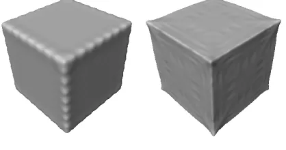
Figure 1 is a synthetic example of the reconstruction of a cube from 770 sample points. 3D surface constraints were uniformly sampled from a cube of dimensions2:0

2:02:0. Values of Æ = 5:0 and = 0:05were used

in the reconstruction to span the average distance of 0.19 between sample points. The reconstruction using isotropic basis functions is shown on the left, while the reconstruction on the right was created using anisotropic basis functions. The isotropic function is radially symmetric and produces a rounded surface even at corner points. In contrast, the anisotropic basis is able to reproduce sharp edges and cor-ners. Notice how the anisotropic basis provides more sup-port along an edge than across it, while the basis at the cen-ter of the cube faces behave isotropically. The reconstruc-tion using the anisotropic basis exhibits sharper corners and edges, and more faithfully reproduces the polygonal cube.

Figure 1. Isotropic (left) and anisotropic (right) reconstructions of a synthetic cube from 770 point samples using values of Æ = 5:0and =0:05.

As shown in Figure 1, the direction of the anisotropy is essential to the reconstruction. In the next section, we discuss how we determine the direction of anisotropy using principle component analysis.

4

Direction of Anisotropy

In order to determine whether a surface point,~p, is part

of a planar region, part of an edge, or occurs at a corner, we look at the number of dominant principle axes spanned by the neighborhood of points~v

iwithin radius

rof~p. To

iden-tify the principle axes of of the local data set, we perform eigenvalue decomposition of the covariance matrix. The co-variance matrix,C(~p ), is a33symmetric tensor that

de-scribes the distribution of points in the neighborhood, and

is computed as the sum of the outer product between each surface point (minus the centroid of the neighborhood) and its transpose:

C(~p)= n X

i=1 (~v

i ~c )(~v

i ~c)

T

(10)

In the above equation,nis the number of points in the

neighborhood. Each~v

i is the location of a surface point

in the neighborhood, and ~c is the centroid of the

neigh-borhood. Our application of principle component analysis differs from that used by Lee, Tang and Medioni in tensor voting [17, 26] and by Hoppe in his surface reconstruction method [14] in that C(~

p ) is not computed using the

esti-mated normal vector of the surface points. Instead, we use the distribution of the local surface points themselves. Ro-bust estimation of the surface normal at the sample points requires that the data set be very precise, which we do not assume in our approach.

The resulting eigenvectors ofC are the three principle

axes of the set of points in the neighborhood. The eigenval-ues indicate the strength of the corresponding eigenvector and help characterize the local point set. When all three eigenvalues are nearly equal, then there is no one or two dominant axes along which all the points span. In such a case, the point set within the neighborhood is likely to be a corner, as long as the local point set is a thin-shelled surface. If there is one strong eigenvalue, then there is one dominant principle axis, and all the points in the neighborhood span that axis. Such a situation is likely to occur along edges, and the dominant axis is the orientation of the edge. If all the points lie on a plane, then they span the space of two vectors (or axes). In such a case, there will be two eigenval-ues that are nearly equal and larger than the third. The two corresponding eigenvectors form the plane along which the points span, and the eigenvector corresponding to the weak-est eigenvalue is the weak-estimated normal vector to the plane.

Once the surface points have been characterized as part of a planar region, part of an edge, or at a corner, the non-uniform scaling is applied to the basis function as described in Section 3 so that it behaves anisotropically. In particu-lar, for an edge point, the direction of anisotropy is aligned with the dominant principle axis. The scaling function,M,

of Equation 9 is applied to the vector between the edge point and an arbitrary point in 3D space to be evaluated, denoted by~

x ~

cin Equation 9. The scaling function contracts the

vector in the direction of the principle axis by a factor of

0:5the ratio between the eigenvalues associated with the

minor axis and the major axis. This contraction causes the basis function in Equations 7 and 8 to be evaluated at a smaller radius than before scaling. Since the basis,(r),

approaches zero asr increases, a smallerrevaluates to a

larger basis value. Hence, the anisotropic basis approaches zero less rapidly in the direction of the principle axis, but more rapidly across the edge which is orthogonal to the principle axis.

4.1

Filtering the Tensor Field

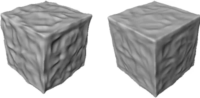
Each covariance matrix, defined by Equation 10 is a ten-sor. We obtain a field of tensors over the entire surface by performing the principle component analysis on each sur-face point in the voxel coloring data set (not just the sursur-face constraints that we uniformly sample as described later in Section 5.1). Principle component analysis is sensitive to noise in the data. For example, if a neighborhood of points is not a thin-shelled surface due to noise, then the catego-rization of the surface point by the method described in the previous section may be incorrect. In addition, the juxtapo-sition of very different tensors will often result in a rough or wrinkled surface. Figure 2 are reconstructions of a syn-thetic example of a cube whose surface points have been in-jected with uniform noise that deviates from the noise-free surface by up to ten percent of the cube dimensions. The left panel of Figure 2 shows the reconstruction of the noisy cube using the anisotropic, multi-order basis without addi-tional filtering of the tensor field. The edges and corners are fairly sharp, but the faces are quite rough.

In order to combat the noise present in the tensor field, we apply a low pass filtering of the tensors using a Gaussian-like kernel. We position the kernel at each surface point. The resulting tensor at the center of the filter is the summation of weighted tensors of all surface points within the support of the filter. Additionally, we modify the support of the filter so that it is anisotropic. We align the filter so that it has greater support along the dominant principle axis of the original tensor at the surface point. This anisotropy has little effect for points in planar regions since the tensors at such points do not have one dominant principle axis, and thus, the support is equal along both dominant axes. The weight of a neighboring tensor is dependent on the distance of the neighboring surface point to the center of the filter. This distance is applied to the anisotropic Gaussian kernel to obtain the weight for the unfiltered tensor. The filtered tensor,C

0 (~p

i

), at a surface point,~p

i, is as follows:

C 0

(~p i

)= P

n j=1

w ij

C(~p j

) P

n j=1

w ij

(11)

w ij

=e j~p

i ~p

j j

2

2r (12)

In the above equation,nis the number of surface points

within the filter radiusr;~p

jare the coordinates of the

sur-face points; andC(~ p j

)is the unfiltered tensor of ~ p

j. The

right panel of Figure 2 shows the reconstruction of the noisy cube after tensor filtering.

4.2

Basis, Neighborhood, and Filter Radii

The span of the basis function, the neighborhood ra-dius used in calculating the unfiltered tensor at each surface point, and the filter radius are all dependent on the sampling density of the data set. The basis function needs to be large enough to span the samples. For noisy data sets, the radius

Figure 2. Reconstructions of the noisy cube without tensor filtering (left) and with tensor filtering (right).

for calculating the tensor at each surface constraint needs to be large in order to be insensitive to the noise. For example, voxel coloring data sets tend to be aliased due to voxeliza-tion. A radius of four or more voxels is required to avoid biases due to the voxelization. The filter radius depends on the noise level of the initial tensors at each surface point. We have used a radius of 0.6 to calculate the initial tensors and a filter radius of 0.4 for the synthetic data set sampled from a2:02:02:0cube injected with uniform noise that

deviates up to 0.2 away from the noise-free surface.

5

Results

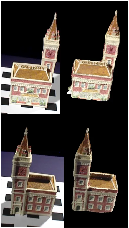
We have applied our approach of surface reconstruction using anisotropic basis functions to a real data set obtained through generalized voxel coloring [7]. The data set is an eight inch tall, souvenir model of Ghirardelli Square. Figure 4 shows actual images of the model. The thin-shelled, vol-umetric data set consists of 72,101 surface voxels, carved from a volume of168104256voxels using 17 images.

5.1

Constraints from Voxel Coloring Data

The generalized voxel coloring algorithm is a space carv-ing approach that begins with a 3D volume and a set of im-ages from arbitrary viewpoints around the object to be re-constructed [7]. Voxels are carved out of the initial volume by splatting each voxel towards each camera and determin-ing the consistency of the voxel color across the images. If the variance in color intensity is below a specified threshold, the voxel is kept as part of the object surface. Otherwise, it is cast out and assigned a zero value. The resulting data is a thin-shelled, volumetric representation of the surface, and consists of red, green, and blue channels for each voxel.

Figure 3. Voxel coloring data set of the eight inch Ghirardelli Square model (left) and the 2000 surface points used in reconstructing the variational implicit surface (right).

results show that this reduced data set is sufficient to gener-ate detailed surfaces using our reconstruction algorithm. In selecting constraints, we use the method described in [9] to uniformly sample the surface, interior, and exterior regions of the object. This method is based on the notion of free

space as introduced in [8]. Free space is the region of space

swept out by the collection of rays emanating from a camera towards surface points visible from that camera. Using the a priori information about the cameras used in generating the voxel coloring data set, we can define exterior points all around the object. Surface points are defined by the voxel coloring data set itself. Interior points are determined by traversing the volumetric data set along each major axis. During the traversal, all points occurring between pairs of surface voxels are marked as interior. Only voxels which are marked as interior by two or more traversals are kept as interior constraints. The left panel in Figure 3 shows the entire voxel coloring data set, and the right panel shows the 2000 surface constraints that were uniformly sampled from the data set and used in the anisotropic variational implicit surface reconstruction.

5.2

Reconstructions

The voxel coloring data set, shown in Figure 3, is aliased due to voxelization and contains floating surface points due to noise and non-textured regions of the model. We have extracted the largest single connected component to remove the floating voxels. We uniformly sample the surface, inte-rior, and exterior to obtain 2000 surface, 50 inteinte-rior, and 200 exterior constraints. All constraints were centered and nor-malized so that the reconstructed model is within a bound-ing box spannbound-ing -1.0 to 1.0 along each axis.

Figure 4. Actual images of the Ghiradelli sou-venir model (left), and reconstructed model rendered at the same camera viewpoints (right).

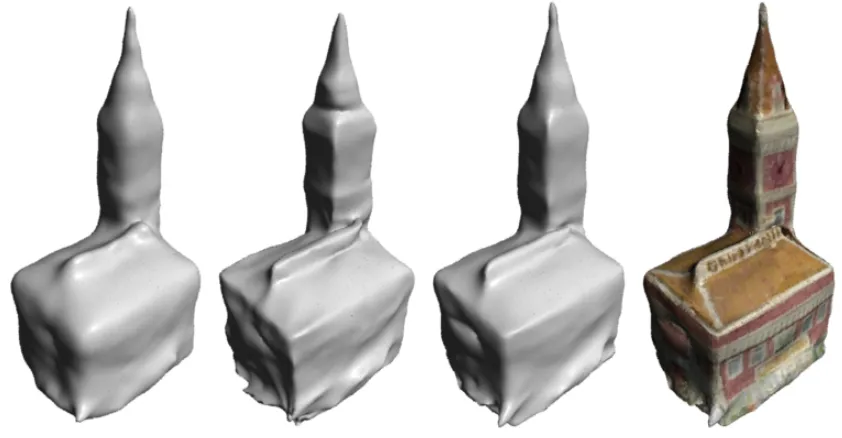
Figure 5 is a comparison of reconstructions using the isotropic basis(left panel), using the anisotropic basis with-out tensor filtering (second panel), and using the anisotropic basis with tensor filtering (third panel). The last panel is a textured version of the reconstruction shown in the third panel. In all four reconstructions,= 0:001at sharp

fea-tures and=0:01in planar regions,Æ =10:0, =0:01,

the neighborhood radius for the initial tensors is 8.0, and the filtering radius when tensor filter was used is 8.0. The av-erage Euclidean distance error measured on all four models from a random sampling of 10,000 surface points are 0.0137 for the isotropic reconstruction, 0.0123 for the anisotropic reconstruction without tensor filtering, and 0.0120 for the anisotropic reconstruction with tensor filtering.

Visually, the reconstructions using an anisotropic basis with tensor filtering (shown in the third and fourth panels)

Figure 5. Comparison of reconstructions using isotropic basis (first), using anisotropic basis without additional tensor field filtering (second), using anisotroipic basis with additional tensor filtering (third), and the final textured reconstruction (fourth). In all four reconstructions,=0:001for surface

points at an edge or corner, and=0:01for planar points.

are the best at capturing sharp features while smoothing out planar regions of the model. The differences between the reconstructions using the isotropic (first panel) versus the anisotropic basis is especially apparent at the edges and corners. The isotropic reconstruction has rounded edges and corners, while those of the anisotropic reconstruction are sharp and well-defined. The differences between the unfiltered (second panel) and filtered (third panel) recon-structions using the anisotropic basis is quite subtle. It is clear, however, that the planar regions of the unfiltered re-construction are more wrinkled. This is also evident in the average error measurements, which show a larger difference between the isotropic and anisotropic reconstructions than between the filtered and unfiltered reconstructions. The er-ror measurements do, however, support the visual notion that the reconstruction using the anisotropic basis with ten-sor filtering is the best of the three, the reconstruction using the anisotropic basis without additional filtering is a close second best, and the reconstruction using the isotropic basis is the worst of the three types of reconstructions.

The final step in our reconstruction is to texture the re-constructed model. We first extract a polygonal model from the implicit surface using Marching Cubes [18]. The polyg-onal model is then subdivided until all triangles of the mesh project to less than a pixel in area for all the input images. We assign color to each triangle of the polygonal model by projecting each triangle to the input image whose cor-responding camera has the best unobscured view of the tri-angle. Typically several cameras will have an unobscured

view of any one triangle, but the one with the best view is the one that has a view most nearly parallel to the trian-gle normal. This is determined by taking the dot product between the triangle normal vector and the view direction vector of the camera. Finally to reduce aliasing, we fil-ter the color of each triangle by taking the average of the colors of the triangle and its neighbors. Figure 4 is a com-parison of two of the original images used in voxel color-ing with the textured reconstruction uscolor-ing anisotropic basis functions. The last panel of Figure 5 shows the textured reconstruction from a novel viewpoint.

6

Conclusion and Future Work

cor-ners better than isotropic reconstruction, and succeeds in smoothing planar regions.

We are currently looking at improved methods for filter-ing the tensor field, includfilter-ing anisotropic diffusion. Addi-tionally, we are looking into potential methods for incor-porating the variational implicit surface approach into the space carving algorithm. Currently, there is no notion of a surface as voxels are carved away. Voxels are kept as a surface voxel only if its color is consistent with the images of the object. We propose that the reconstructed surface be used as an additional guide in rejecting voxels and in refin-ing the threshold variance above which voxels are rejected.

7

Acknowledgements

We thank James O’Brien for stimulating discussions about alternate basis functions for surface creation. We also acknowledge Bruce Culbertson, and Tom Malzbender of

Hewlett-Packard for use of the generalized voxel coloring

algorithm. This work was funded by the Graphics,

Visu-alization, and Usability Center Seed Grant in collaboration

with Ronald Schafer of the Center for Signal and Image

Processing, Georgia Institute of Technology.

References

[1] Amenta, N., M. Bern, and M.Kamvysselis. A New Voronoi-Based Surface Reconstruction Algorithm. SIGGRAPH Proceedings, Aug. 1998, pp. 415–420.

[2] Bajaj, C. L., F. Bernardini, and G. Xu. Automatic Reconstruction of Surfaces and Scalar Fields from 3D Scans. SIGGRAPH Proceedings, Aug. 1995, pp. 109–118.

[3] Bernardini, F., J. Mittleman, H. Rushmeier, and C. Silva. The Ball-Pivoting Algorithm for Surface Reconstruction. IEEE Transactions

on Visualization and Computer Graphics, 5(4), Oct.-Dec. 1999, pp.

349–359.

[4] Blinn, J. A Generalization of Algebraic Surface Drawing. ACM

Transactions on Graphics, 1(3), July 1982, pp. 135–256.

[5] Boult, T.E. and J.R.Kender. Visual Surface Reconstruction Using Sparse Depth Data. Computer Vision and Pattern Recognition

Pro-ceedings, 1986, pp. 68–76.

[6] Chen, F. and D. Suter. Multiple Order Laplacian Spline - Includ-ing Splines with Tension. MECSE 1996-5, Dept. of Electrical and

Computer Systems Engineering Technical Report, Monash Univer-sity, July 1996.

[7] Culbertson, W. B., T. Malzbender, and G. G. Slabaugh. Generalized Voxel Coloring. Vision Algorithms: Theory and Practice. Part of Se-ries: Lecture Notes in Computer Science, 1883, Sept. 1999, pp. 67– 74.

[8] Curless, B. and M. Levoy. A Volumetric Method for Building Com-plex Models from Range Images. SIGGRAPH Proceedings, Aug. 1996, pp. 303–312.

[9] Dinh, H. and G. Turk. Reconstructing Surfaces by Volumetric Regu-larization. Technical Report 00-26, Graphics, Visualization, and

Us-ability, Georgia Institute of Technology, November, 2000.

[10] Edelsbrunner H. and E.P. Mucke. Three-Dimensional Alpha Shapes.

ACM Transactions on Graphics, 13(1), Jan. 1994, pp. 43–72.

[11] Fang, L. and D. Gossard. Multidimensional Curve Fitting to Unorga-nized Data Points by Nonlinear Minimization. Computer-Aided

De-sign, 27(1), Jan. 1995, pp. 48–58.

[12] Faugeras, O. and R. Keriven. Complete Dense Stereovision Using Level Set Methods. Proceedings Fifth European Conference on

Com-puter Vision, 1998.

[13] Girosi, F., M. Jones, and T. Poggio. Priors, Stabilizers and Ba-sis Functions: From Regularization to Radial, Tensor and Additive Splines A.I. Memo No. 1430, C.B.C.L. Paper No.75, Massachusetts

Institute of Technology Artificial Intelligence Lab, June, 1993.

[14] Hoppe, H., T. DeRose, and T. Duchamp. Surface Reconstruction from Unorganized Points. SIGGRAPH Proceedings, July 1992, pp. 71–78.

[15] Keren, D. and C. Gotsman. Fitting Curve and Surfaces with Con-strained Implicit Polynomials. IEEE Transactions on Pattern

Analy-sis and Machine Intelligence, 21(1), pp. 21–31, 1999.

[16] Kutulakos, K.N. and S.M.Seitz. A Theory of Shape by Space Carv-ing. International Journal of Computer Vision, 38(3), July 2000, pp. 198–218.

[17] Lee, M. and G. Medioni. Inferring Segmented Surface Description from Stereo Data. Computer Vision and Pattern Recognition

Proceed-ings, 1998, pp. 346–352.

[18] Lorensen, W.E. and H.E. Cline. Marching Cubes. SIGGRAPH

Pro-ceedings, July 1987, pp. 163–169.

[19] Malladi, R., J.A. Sethian, and B.C. Vemuri. Shape Modeling with Front Propagation: A Level Set Approach. IEEE Transactions on

Pat-tern Analysis and Machine Intelligence, 17(2), Feb. 1995.

[20] Muraki, S. Volumetric Shape Description of Range Data Using Blobby Model. SIGGRAPH Proceedings, 1991, pp. 227–235.

[21] Pentland, A. Automatic Extraction of Deformable Part Models.

In-ternational Journal of Computer Vision, Vol.4, 1990. pp.107–126.

[22] Savchenko, V.V., A.A. Pasko, O.G.Okunev, and T.L.Kunii. Func-tion RepresentaFunc-tion of Solids Reconstructed from Scattered Surface Points and Contours. Computer Graphics Forum, Vol. 14, No. 4, 1995, pp.181– 188.

[23] Sclaroff, S. and A. Pentland. Generalized Implicit Functions for Computer Graphics. SIGGRAPH Proceedings, July 1991, pp.247– 250.

[24] Seitz, S.M. and C.R. Dyer. Photorealistic Scene Reconstruction by Voxel Coloring. International Journal of Computer Vision, 35(2), 1999, pp. 151–173.

[25] Suter, D. and F, Chen. Left Ventricular Motion Reconstruction Based on Elastic Vector Splines. To appear in IEEE Transactions on Medical

Imaging, 2000.

[26] Tang, C. and G. Medioni. Inference of Integrated Surface, Curve, and Junction Descriptions From Sparse 3D Data. IEEE Transactions

on Pattern Analysis and Machine Intelligence, 20(11), Nov. 1998.

[27] Taubin, G. An Improved Algorithm for Algebraic Curve and Surface Fitting. Proceedings Fourth International Conference on Computer

Vision, May 1993, pp. 658–665.

[28] Terzopoulos, D. The Computation of Visible- Surface Representa-tions. IEEE Transactions on Pattern Analysis and Machine

Intelli-gence, 10(4), July 1988.

[29] Terzopoulos, D. and D. Metaxas. Dynamic 3D Models with Local and Global Deformations: Deformable Superquadrics. IEEE

Trans-actions on Pattern Analysis and Machine Intelligence, Vol. 13, No. 7,

July, 1991.

[30] Turk, G. and J.F. O’Brien. Shape Transformation Using Variational Implicit Functions. SIGGRAPH Proceedings, Aug. 1999, pp. 335– 342.

[31] Yngve, G. and G. Turk. Creating Smooth Implicit Surfaces from Polygonal Meshes. Technical Report 99-42, Graphics, Visualization,

and Usability, Georgia Institute of Technology, 1999.