P Karagiannakis
∗, K Thompson
∗, J Corr
∗, IK Proudler
†, S Weiss
∗∗Department of Electronic and Electrical Engineering, University of Strathclyde, Glasgow, Scotland
†School of Electronic, Electrical and Systems Engineering, Loughborough University, Loughborough, UK
{philipp.karagiannakis,keith.thompson,stephan.weiss}@strath.ac.uk
Abstract. Fractals have been proven as potential candidates for satellite flying formations, where its different elements represent a thinned array. The distributed and low power nature of the nodes in this network motivates distributed processing when using such an array as a beamformer. This paper proposes such initial idea, and demonstrates that benefits such as strictly limited local processing capability independent of the array’s dimension and local calibration can be bought at the expense of a slightly increased overall cost.
1. Introduction
Recent work established a Purina fractal geometry as a forma-tion of fracforma-tionated spacecraft as an alternative to larger satel-lites [1,2]. Additionally, the Purina fractal’s structural sparse-ness combines a significant aperture and therefore resolution while avoiding spatial aliasing as long as at least some sen-sors are sufficiently closely located [3–6], thus offering advan-tages that otherwise have to be achieved through thinning of arrays [7,8].
In order to exploit the fractionated nature of a satellite as proposed in [2], we aim to mirror its fractal structure in the processing architecture, since the lack of a central process-ing node motivates the design of a distributed beamformer. In the past such efforts have e.g. concentrated on the dis-tributed estimation of the covariance matrix [9], disdis-tributed signal enhancement with bandwidth constraints [10] or the use of factor graphs [11] and specifically Pearl’s algorithm [12], which could lead to the implementation of general algorithms in a distributed fashion. Some distributed algorithms have also been developed for spatially separated subarrays [13,14] with the main emphasis on the iterative approximation of jointly optimal results.
Our aim here is to use a hierarchical distributed processing structure which closely mirrors the fractal architecture of the array. In particular, we propose to use nested subarrays, whereby a subarray takes the shape of the generating frac-tal. The beamformer output can be hierarchically computed such that, independent of the dimension of the Purina array, the number of computations per node are strictly limited, even though the overall number of computations is slightly increased compared to directly processing the samples col-lected by all sensors.
Below, we first review characteristics and the generation of the Purina fractal array in Sec. 2.. The beamformer output, its qui-escent response, and its distributed computation are outlined in Sec. 3., while some results and discussions are provided in
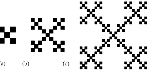
[image:1.595.307.555.310.426.2](a) (b) (c)
Figure 1. First three stages of growth of the Purina fractal array for (a)P=1, (b)P=2, and (c)P=3.
Sec. 4.. Finally, conclusions are drawn in Sec. 5..
2. Purina Fractal Array
2.1 Purina Array Generation
The Purina fractal pattern yields a thinned 3-by-3 symmetric planar array, which at growth stageP=1 has the simple sub-array S1
S1=
1 0 1 0 1 0 1 0 1
, (1)
also referred to as the generating array. Higher growth stages
P∈N,P>1 are defined recursively by
SP=S1⊗SP−1 , (2)
with⊗denoting the Kronecker product, whereby a unit entry means that an element is switched on, while zero indicates that the array element is switched off. Fig. 1 demonstrates the first three stages of growth for the Purina fractal array.
2.2 Hierarchy and Labelling
r2 r3
r1
r5 r4
r3,2 r3,3
r3,1=r3
r3,5 r3,4
r3,4,2 r3,4,3
r3,4,1=r3,4
[image:2.595.138.474.90.195.2]r3,4,5 r3,4,4
Figure 2. Nested labelling of array elements at fractal scalep=1 with sensor locationsrk, fractal scalep=2 with locationsrk,l, and fractal scalep=3 with
locationsrk,l,m, withk,l,m∈ {1...5}.
stageP. The elements at the coarsest level,p=1, are given a single index, elements at fractal scalep=2 a double index, and so on, until the elements at the finest scalep=Pare labelled using P subscripts. For the three coarsest levels of a Purina fractal array, an example is provided in Fig. 2. Note that in gen-eral,
rk,l,...,r,q,1=rk,l,...,r,q , (3) and in particular
r1,1,...,1,1=r1,1,...,1=· · ·=r1 . (4)
Using these sensor locations, below we will be able to define a distributed beamforming system exploiting the fractal scale structure of the Purina array, by labelling the narrowband beamforming coefficient and the data sample collected at time instancenin the sensor location denoted by a vectorrk,l,...,p,q aswk,l,...,p,qandxk,l,...,p,q[n], respectively.
3. Distributed Beamformer
This section derives a beamformer formulation for using dis-tributed processing of inputs based on the definition of the beamformer output in Sec. 3.1 and its coefficients for the qui-escent case in Sec. 3.2. A restructuring of the equations in Sec. 3.3 yields a formulation with a slightly increased cost, which however allows to calibrate information that is only available within subarrays.
3.1 Beamformer Output
The overall beamformer response is given by
y[n] = wHx[n] (5)
=
5
∑
uP=1· · ·
5
∑
u2=15
∑
u1=1| {z }
P terms
wuP,...u2,u1xuP,...,u2,u1[n] , (6)
wherebywandx[n]are the stacked coefficient and data vectors at timen,{·}Hdenotes Hermitian transpose. The computations
that are required for one output sampley[n]are constituted by 5P multiply-accumulate operation, that would under normal circumstances be executed in a central processing node. Inter-estingly, the nesting of the summation terms in (6) provides a
natural hierarchy in calculating the output, whereby intermedi-ate outputs of nested subarrays are defined as
y[n] =
5
∑
uP=1yuP[n] (7)
.. .
=
5
∑
uP=1· · ·
5
∑
u2=1yuP,...,u2[n] (8)
=
5
∑
uP=1· · ·
5
∑
u2=15
∑
u1=1yuP,...,u2,u1[n] . (9)
The quantities under the sum on the r.h.s. of (9) denote the out-put of subarrays at different fractal scales of the array, such thatyP[n]are the outputs at the 5 nodes at the coarsest level as shown on the left side of Fig. 2, and outputs with an increas-ing number of subscripts refer to intermediate outputs at finer fractal scales.
3.2 Quiescent Beamformer Coefficients
Assuming a far field source at a narrowband frequencyf which arrives at the array as a planar wave front with normal vectork,
kϕ,ϑ =
cosϕsinϑ
sinϕsinϑ
cosϑ
, (10)
i.e. with azimuthϕ and elevation angleϑ, the relative time delay τuP,...u2,u1 experienced at location ruP,...,u2,u1 relative to
the centre element atr1is given by
τuP,...,u2,u1=
1
ck T
ϕ,ϑ(ruP,...,u2,u1−r1) (11)
with c denoting the propagation speed in the medium. The quantity kϕ,ϑ/cis also known as the slowness vector of the source.
charac-terised by a steering vectorsϕ,ϑ,
sϕ,ϑ =
e−jΩτ1,...,1,1
.. .
e−jΩτ1,...,1,5 e−jΩτ1,...,2,1
.. .
e−jΩτ5,...,5,5
, (12)
withΩ=2πf/fs. For the quiescent case, (12) defines the opti-mum filter coefficientsw=s∗ϕ,ϑ, i.e. the matched filter, in the mean square error sense.
3.3 Distributed Processing with Local Calibration
On the finest fractal scale, different from (11) we define the time shift relative to the centre of a subarray,
˜
τuP,...,u2,u1=
1
ck T
ϕ,ϑ(ruP,...,u2,u1−ruP,...,u2) . (13)
Therefore, 5P−1steering vectors ˜s
uP,...,u2|ϕ,ϑ∈C 5,
˜ su
P,...,u2|ϕ,ϑ =
1
e−jΩτ˜uP,...,u2,2
.. .
e−jΩτ˜uP,...,u2,5
(14)
emerge at the finest scale. The time delays can therefore be adjusted based on local knowledge of the actual locations ruP,...,u2,u1 within each subarray.
At the next coarser level, 5P−2 groups of steering vectors ˜
suP,...,u3|ϕ,ϑ ∈C25 are assembled by weighting contributions
of the sub-steering vectors in (14). This weighting reflects the calibration w.r.t. the time difference at this fractal scale,
˜
suP,...,u3|ϕ,ϑ=
˜ suP,...,u
3,1|ϕ,ϑ e−jΩτ˜uP,...,u3,2s˜
uP,...,u3,2|ϕ,ϑ
.. .
e−jΩτ˜uP,...,u3,5s˜
uP,...,u3,5|ϕ,ϑ
, (15)
whereby the time delays ˜τuP,...,u3,u2 represent calibrations
w.r.t. the central nodes of the next finer fractal scale,
˜
τuP,...,u3,u2=
1
ck T
ϕ,ϑ(ruP,...,u3,u2−ruP,...,u3) . (16)
The process of (14) and (15) can be iterated until the coarsest fractal scalep=1 is reached.
At the coarsest fractal scalep=1, finally the complete steering vector
sϕ,ϑ=
˜ s1|ϕ,ϑ
e−jΩτ˜2s˜ 2|ϕ,ϑ .. .
e−jΩτ˜5s˜ 5|ϕ,ϑ
, (17)
1 1.5 2 2.5 3 3.5 4 4.5 5
101 102 103
growth scaleP
co m p le x it y C , ˜C
distributed, ˜C
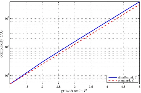
[image:3.595.309.552.97.257.2]standard,C
Figure 3. Complexity for standard (C) and distributed processing ( ˜C) as a function of the growth stageP.
with
˜
τup= 1
ck T
ϕ,ϑ(ruP−r1) (18) is obtained, which matches the original steering vectorsϕ,ϑ ∈
C5P in (12).
The computational structure in calculating the output (9) can be performed to match the nested iterative structure of steering vectors presented by (14), (15) and (17). At the finest scale, outputs ˜yuP,...,u3,u2[n]are determined as
˜
yuP,...,u3,u2[n] = 5
∑
u1=1˜
wuP,...,u2,u1·xuP,...,u2,u1[n] , (19)
with the coefficients ˜wuP,...,u2,u1matched to the modified
steer-ing vectors ˜su
P,...,u2|ϕ,ϑin (14). From this finest level upwards,
at each fractal scale phase corrections as in (15) and (17) are applied when adding up outputs in a divide-and-conquer fash-ion to finally reachy[n]at the coarsest fractal scale.
4. Discussion, Simulations and Results
4.1 Computational Complexity
The complexity of the direct formulation in (6) via a scalar product requiresC=5P multiply-accumulates, which might need to be afforded in a central processing node, where data, weights, and any calibration for displaced sensors might be required. For the proposed computational structure in Sec. 3.3, the hierachical processing structure requires a total of
˜
C=
P
∑
p=15p>C . (20)
−80 −60 −40 −20 0 20 40 60 80 −40
−35 −30 −25 −20 −15 −10 −5 0 5
ϑ/[◦]
10
lo
g10
|
DP
(
ϑ
,ϕ
=
0)
|
/
[d
B
]
[image:4.595.52.297.95.309.2]P=1 P=2 P=3 P=4
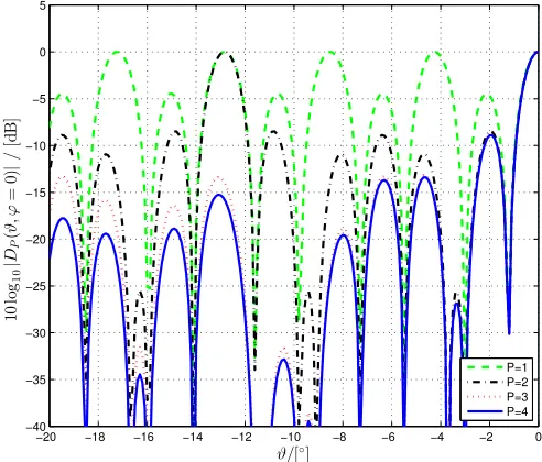
Figure 4. Quiescent beampatterns of Purina array for different growth stages
P=1, 2, 3 and 4, assuming that in each case the array elements’ minimum spacing satisfies spatial sampling.
−35 −30 −25 −20 −15 −10 −5 0
−40 −35 −30 −25 −20 −15 −10 −5 0 5
ϑ/[◦]
10
lo
g1
0
|
DP
(
ϑ
,ϕ
=
0)
|
/
[d
B
]
P=1 P=2 P=3 P=4
Figure 5. Detail view of Fig. 4, showing the main beam forP=1 and the iterative inscribed characteristics for finer fractal scaled Purina fractal arrays.
structure is easier to calibrate, as dislocations of sensors only have to be known at the local subarray level, which matches the control strategy for flying a Purina array in formation, as outlined in [3].
4.2 Beampatterns
A number of sample beampatterns for the Purina array beam-former are shown in Figs. 4 and 5. These beampatterns emerge from a beamformerDP(ϑ,ϕ)matched to receive a signal from broadside,ϑ=0◦, and are calculated by probing the array with a set of steering vectorssϕ,ϑas defined in (12) for variable
ele-−80 −60 −40 −20 0 20 40 60 80
−40 −35 −30 −25 −20 −15 −10 −5 0 5
ϑ/[◦]
10
lo
g10
|
DP
(
ϑ
,ϕ
=
0)
|
/
[d
B
]
[image:4.595.309.558.97.309.2]P=1 P=2 P=3 P=4
Figure 6. Quiescent beampatterns of Purina array adjusted to sample cor-rectly with growth stageP=4, while processing of finer fractal scales for
p=1, 2, and 3 operate on a subsampled array.
−20 −18 −16 −14 −12 −10 −8 −6 −4 −2 0
−40 −35 −30 −25 −20 −15 −10 −5 0 5
ϑ/[◦]
10
lo
g1
0
|
DP
(
ϑ
,ϕ
=
0)
|
/
[d
B
]
P=1 P=2 P=3 P=4
Figure 7. Detail view of Fig. 6, showing the main beam forP=4 and the iterative inscribed characteristics for coarser fractal scales of the Purina arrays.
vationϑ,
DP(ϑ,ϕ) =wHsϕ,ϑ . (21)
The azimuth is in this case set to zero,ϕ=0◦. Since for every value ofP, the minimum distance between array elements is set to fulfil correct spatial sampling, no aliasing occurs, and an increase in P corresponds to an increase in resolution as characterised by the narrowing beamwidth at ϑ =0◦, and lower sidelobe levels. Note that the fractal structure of the array results in “inscribed” or majorised beampatterns where |DP+1(ϑ,ϕ)|<|DP(ϑ,ϕ)|∀ϑ,ϕ,P.
[image:4.595.312.558.357.567.2] [image:4.595.51.299.357.570.2]sam-pling for the caseP=4, with the beam pattern matching the ones shown in Figs 4 and 5. If only coarser fractal scalesp<P
are processed, subarrays are spatially subsampled and spatial aliasing can be noticed. Interestingly, again the fractal struc-ture of the array results in majorised beampatterns.
5. Conclusions
We have considered distributed processing for a Purina frac-tal array, which emerges from a generating subarray to reach a growth stagePover a number of fractal scalesp=1. . .P. The considered processing consisted of the calculation of a beam-former output, which can exploit the fractal structure to define the distributed processing architecture. As a simple example, we have assumed a quiescent beamformer, which is optimal in a scenario where a single source is embedded in isotropic noise.
The advantages of the discussed processing architecture lie in the fixed maximum complexity per node in the distributed pro-cedure. In addition to limiting the processing power, transmit power is conserved through short hops. Further, the distributed approach matches the position control strategy of the Purina array for formation flying, and allows to consider calibration information in the form of locally known dislocation of sensor elements when computing the beamformer output.
References
[1] J. Leitner, “Formation flying: The future of remote sensing from space,” NASA Tech. Report, Goddard Space Flight Center, MD, Tech. Rep., 2004.
[2] G. Punzo, D. J. . Bennett, and M. Macdonald, “A fractally fractionated spacecraft,” in 62nd International Astronautical Congress, Cape Town, South Africa, October 2011.
[3] G. Punzo, P. Karagiannakis, D. Bennet, M. Macdonald, and S. Weiss, “Enabling and exploiting self-similar central symme-try formations,”IEEE Transaction on Aerospace and Electronic Systems, 2013, (accepted).
[4] D. Werner, R. L. Haupt, and P. Werner, “Fractal antenna engi-neering: the theory and design of fractal antenna arrays,”IEEE Antennas and Propagation Magazine, vol. 41, no. 5, pp. 37–58, October 1999.
[5] P. Karagiannakis, S. Weiss, G. Punzo, M. Macdonald, J. Bow-man, and R. Stewart, “Impact of a Purina fractal array geom-etry on beamforming performance and complexity,” in 21st European Signal Processing Conference, Marrakech, Morocco, September 2013, (to appear).
[6] P. Karagiannakis and S. Weiss, “Analysis of a purina fractal beamformer,” inAsilomar Conference on Signals, Systems and Computers, Pacific Grove, CA, November 2013, (accepted). [7] R. M. Leahy and B. D. Jeffs, “On the Design of Maximally
Sparse Beamforming Arrays,”IEEE Transactions on Antennas and Propagation, vol. 39, no. 8, pp. 1178–1188, August 1991. [8] G. Cardone, G. Cincotti, and M. Pappalardo, “Design of
wide-band arrays for low side-lobe level beam patterns by simulated annealing,”IEEE Transactions on Ultrasonics, Ferroelectrics and Frequency Control, vol. 49, no. 8, pp. 1050–1059, August 2002.
[9] U. Khan and J. M. F. Moura, “Distributing the Kalman filter for large-scale systems,”IEEE Transactions on Signal Processing, vol. 56, no. 10, pp. 4919–4935, November 2008.
[10] A. Bertrand and M. Moonen, “Distributed LCMV beamform-ing in a wireless sensor network with sbeamform-ingle-channel per-node signal transmission,”IEEE Transactions on Signal Processing, vol. 61, no. 13, pp. 3447–3459, 2013.
[11] H.-A. Loeliger, “An introduction to factor graphs,”IEEE Signal Processing Magazine, vol. 21, no. 1, pp. 28–41, January 2004. [12] I. Proudler, S. Roberts, S. Reece, and I. Rezek, “An iterative
signal detection algorithm based on Bayesian belief propaga-tion ideas,” in15th International Conference on Digital Signal Processing, Cardiff, UK, July 2007, pp. 355–358.
[13] K. Zarifi, S. Affes, and A. Ghrayeb, “Distributed processing techniques for beamforming in wireless sensor networks,” in
3rd International Conference on Signals, Circuits and Systems, Medenine, Tunisia, November 2009, pp. 1–5.