Linear matching method for parametric studies of weldments creep-fatigue endurance

Proceedings of the ASME 2013 Pressure Vessels & Piping Division Conference PVP2013 July 14-18, 2013, Paris, France

PVP2013-97221

DRAFT: LINEAR MATCHING METHOD FOR PARAMETRIC STUDIES OF

WELDMENTS CREEP-FATIGUE ENDURANCE

Yevgen Gorash

Department of Mechanical & Aerospace Engineering University of Strathclyde

James Weir Building, 75 Montrose Street Glasgow G1 1XJ, United Kingdom Email: [email protected]

Haofeng Chen∗

Department of Mechanical & Aerospace Engineering University of Strathclyde

James Weir Building, 75 Montrose Street Glasgow G1 1XJ, United Kingdom Email: [email protected]

ABSTRACT

This paper presents parametric studies on creep-fatigue en-durance of the steel AISI type 316N(L) weldments defined as types 1, 2 and 3 according to R5 Vol. 2/3 Procedure classifica-tion at 550◦C. The study is implemented using the Linear Match-ing Method (LMM) and based upon previously developed creep-fatigue evaluation procedure considering time fraction rule. Sev-eral geometrical configurations of weldments with individual pa-rameter sets, representing different fabrication cases, are devel-oped. For each of configurations, the total number of cycles to failure N?in creep-fatigue conditions is assessed numerically for different loading cases. The obtained set of N?is extrapolated by the analytic function dependent on normalised bending mo-ment ˜M, dwell period∆t and geometrical parameters. Proposed function for N?shows good agreement with numerical results ob-tained by the LMM. Therefore, it is used for the identification of Fatigue Strength Reduction Factors (FSRFs) intended for design purposes and dependent on proposed variable parameters.

NOMENCLATURE

∆σ stress range

ε strain

˙

ε strain rate

∆ε strain range

ω damage parameter

t time

t∗ time to pure creep failure ∆t dwell period

E Young’s (elasticity) modulus ¯

E effective elastic modulus

µ Poisson’s ratio

N∗ number of cycles to pure fatigue failure N? number of cycles to creep-fatigue failure L? residual life

˜

M normalised bending moment ∆M bending moment range P normal pressure IX area moment of inertia w,thk width and thickness of plate

α,β,ρ parameters governing the profile form of type 1, 2 and 3 weldments

R1,R2,R3 radiuses of weld profile for type 1, 2 and 3 weldments correspondingly

δ height of weld profile in type 1 weldment D distance between opposite weld surfaces in

type 2 weldment

a width of weld throat in type 3 weldment h1,d1,h2,d2,h3 auxiliary geometrical parameters for type 1,

2 and 3 weldments correspondingly

σy yield stress

B,β R-O model constants

p0,p1,p2 coefficients for parent material S-N curve

INTRODUCTION

According to industrial experience, during the service life of welded structures subjected to cyclic loading at high temper-ature, welded joints are usually considered as the critical loca-tions of potential creep-fatigue failure. This is caused by higher stress concentration, altered and non-uniform material properties of weldments compared to the parent material of the entire struc-ture. Therefore, creep and fatigue characteristics of welded joints are of a priority importance for long-term integrity assessments and design of welded structures. There were attempts to develop analytical tools [1, 2] to estimate long-term strength of welded joints under variable loading. However, residual life assessments are frequently complicated and inaccurate because of complex material microstructure and too many parameters affecting the strength of welded joints. In view of the complexity of a unified model development for the assessment of creep-fatigue strength, there are a limited number of existing analytical approaches, but none of which are able to account for all of weldment parame-ters mentioned above. Thus, long-term strength of weldments is a wide research area, which requires some unified integral ap-proach able to improve the life prediction capability for welded joints. The most comprehensive overviews of studies devoted to investigation of influence of various parameters on fatigue life of welded joints are presented in [1, 2]. However, the influence of creep on residual life is not investigated in these works.

This paper presents further extension of a latest developed approach [3], which includes a creep-fatigue evaluation proce-dure considering time fraction rule for creep-damage assessment and a recent revision of the Linear Matching Method (LMM) to perform a cyclic creep assessment [4]. The applicability of this approach to a creep-fatigue analysis was verified in [3] by the comparison of FEA/LMM predictions for an AISI type 316N(L) steel cruciform weldment at 550◦C with experiments by Brether-ton et al. [5, 6] with the overall objective of identifying fatigue strength reduction factors (FSRF) of austenitic weldments for further design applications. An overview of previous modelling studies devoted to analysis and simulation of these experiments [5, 6] is given in [3]. The parametric study presented in this pa-per is based on the research outcomes given in prior work [3] successfully validated by matching the basic experiments [5, 6]. Thus, exactly the same assessment approach is applied to para-metric studies of the weldment geometry in order to assess the effect on the predicted residual life.

Another outcome of the previous work [3] is the formulation of an analytical function for the total number of cycles to fail-ure N?in creep-fatigue conditions, which is dependent on nor-malised bending moment ˜M and dwell period∆t. This function N?(_M,˜ _{∆t)matches the LMM predictions with reasonable} accu-racy and is used for the investigation of∆t influence on the FSRF. Therefore, the effect of creep on long-term strength of type 2 dressed weldments (according to the classification in R5 Vol. 2/3 Procedure [7]) is taken in to account.

Apart from operational parameters ( ˜M and ∆t), it is neces-sary to investigate the influence of a weld profile geometry on creep-fatigue strength within a parametric study. The introduc-tion of geometrical parameters into the funcintroduc-tion N?(_M,˜ _∆t) al-lows the calculation of the FSRF as a continuous function able to cover a variety of weld profile geometries including type 1, 2 and 3 in dressed, as-welded and intermediate configurations.

PARAMETRIC MODELS OF WELDMENTS Geometrical relations

It has been indicated [1] that one of the most critical fac-tors affecting the creep-fatigue life of a welded joint is the con-sistency of the cross-sectional weld geometry. The simplified weld profile is usually characterised by the following geometric parameters [1]: plate thickness, effective weld throat thickness, weld leg length, weld throat angle, and weld toe radius. Usually, the weld profile is assumed to be circular for type 1, circular or triangular for type 2, and triangular for type 3 weldments with fillets on toes connecting with parent plates. A vast quantity of researches reviewed in [1, 2] has been devoted to investigation of effects produced by geometrical parameters on residual life.

In the present study, the geometry of the weld profiles for type 1, 2 and 3 weldments is more completely specified in or-der to investigate their as-welded, dressed and intermediate con-figurations. The basis of the parametric models for type 1 and 2 weldments shown in Fig. 1 are the sketches of the weldment specimens produced by the Manual Metal Arc (MMA) welding and reported in [5]. The type 1 weldment specimen contains a double-sided V-butt convex-fillet weld, and the type 2 weld-ment specimen contains 2 symmetric double-sided T-butt cruci-form concave-fillet welds. The basis of the parametric model for type 3 weldment shown in Fig. 1 are the sketches of weld pro-files and corresponding regulations from British Standards [8, 9] for the weldment, which contains a root gap between the parts to be joined. The type 3 weldment specimen contains 2 symmetric double-sided T-butt cruciform mitre-fillet welds.

The parent material for the manufacturing of all specimens are continuous plates of width w=200 mm and thickness thk= 26 mm made of the steel type AISI 316N(L). The typical division of the weld into three regions is adopted here analogically to [3] including: parent material, weld metal and heat-affected zone (HAZ). It should be noted that the HAZ thickness is assumed to be 3mm based on the geometry given in [5]. These 3 regions have different mechanical properties described by the following material behaviour models and corresponding constants at 550◦C in [3] for the FEA with the LMM:

• Elastic-perfectly-plastic (EPP) model for the design limits as a result of shakedown analysis;

R2

thk 60°

h2

haz

α

D

β

α

thk

40°

haz α α

M

M

M

type 2

type 1

R1

δ

d2

h2

h1

d1

thk 2

thk

45°

haz a

haz

5°

45° R

3

h3

thk 2

type 3

M

TIG dressing

FIG. 1 WELD PROFILE GEOMETRIES OF TYPES 1, 2

AND 3 WELDMENTS ACCORDING TO R5 [7]

• S–N diagrams for the number of cycles to failure caused by pure low-cycle fatigue (LCF);

• Power-law model in “time hardening” form for creep strains during primary creep stage;

• Reverse power-law relation for the time to creep rupture caused by creep relaxation during dwells;

• Non-linear diagrams for creep-fatigue damage interaction for the estimation of total damage.

The profile geometry of type 2 weldment is comprehensively characterised by one of two pairs of parameters: (1) independent parameters (αandβ), which are not dependent on a plate thick-ness thk, and (2) technologically controlled parameters (R2and

D), which change their values with a change of plate thickness thk. In parametric relations for strength of type 2 weldments the independent parameters (α andβ) are used with a capabil-ity of transformation into controlled parameters (R2and D). As illustrated in Fig. 1, angleα represents a local geometrical non-uniformity caused by a deviation from the tangent condition be-tween parent plate and weld. Angleβ represents a global geo-metrical non-uniformity caused by deposition of weld metal con-necting the orthogonal part.

The relations between the two parameter pairs (α,βand R2,

D) for a type 2 weldment are formulated using basic trigonomet-ric calculus in conjunction with the thickness of a plate cross-section thk and the corresponding associated parameters (h2and

d2) as illustrated in Fig. 1:

h2=

thk

8.6666 and d2= thk

2 +h2+

thk−h2 2 tan 60

◦_{. (1)}

The direct transitions are formulated as follows

R2=

thk/2 cos(α+β)−

d2 sin(α+β) sinα

sin(α+β)−

cosα cos(α+β)

and

D=2R2cosα+thk/2 cos(α+β) −2 R2.

(2)

The reverse transitions are formulated as follows

β=arccos "

d₂2+ (thk/2)2−R2₂−(R2+D/2)2

−2 R2(R2+D/2)

# ,

α=90◦−arctan _thk

2 d2

−β

−arccos 



R2₂−(R2+D/2)2−d22−(thk/2) 2

−2(R2+D/2)

q

d₂2−(thk/2)2 

. (3)

Relations between independent parameterα and controlled parameter δ for type 1 weldment are formulated using basic trigonometric calculus in conjunction with the thickness of a plate cross-section thk and the corresponding associated param-eters (h1and d1) as illustrated in Fig. 1:

h1=

thk

13 and d1=

thk−h1 2 tan 40

The direct transition is formulated as follows

δ =R1(1−cosα) with R1=d1/sinα. (5)

The reverse transition is formulated as follows

α=arccos _R

1−δ

R1

with R1=δ 2+

d2₁

2δ. (6)

Since the geometry of type 3 weldment profile due to mitre fillet is much simpler than the geometry of type 1 and 2 weld-ments, there are only a few parameters governing this type of geometry. The form of type 3 weld is a isosceles triangle with right angle, as shown in Fig. 1. It is characterised by the weld throat a, which should be(a≥0.7 thk)according to the stan-dard [8]. The gap between the welded parts h3should satisfy the requirement(h3≤1 mm+0.3 mm a), but it shouldn’t exceed 4 mm according to the standard [9].

The fatigue performance of the original type 3 weld profile is quite poor due to significant stress concentration in the weld toe caused by inconsistency of weld profile in 135◦. Moreover, the gap between the welded parts decreases the effective cross-section limiting it to the only area of weld metal. For the purpose of the fatigue life improvement, different post weld treatment techniques are applied to the weld toe, as a potential location of failure. TIG dressing was found in [10] to be the best suited post weld treatment for implementation in mass production compared to burr grinding and ultrasonic impact treatment, because of the large improvement observed in the experiments (up to 40% in-crease in fatigue strength). Therefore, R3in Fig. 1 is the radius of fillet produced by TIG dressing on the weld toe. The angle of discrepancy for the tangency condition between TIG weld metal and patent plate is 5◦, since it is a minimum allowable angle for a finite element in order not to be distorted.

Since the proposed parameters for type 1 and 2 weld profiles are fully convertible, they can be used to characterise different scales of technological dressing of weldments by grinding such as dressed, as-welded and intermediate. Thus, in order to reduce the computational costs, only five configurations of weld profile, listed in Table 1, were chosen for parametric study from among the possible parameter combinations. In case of type 3 weld-ment, the different scales of TIG dressing are characterised by the parameter ratioρbetween fillet radius and plate thickness:

ρ=R3/thk. (7)

Analogically to Table 1, seven configurations are proposed for the parametric study of type 3 weldment described by the following values of the parameterρ: 2.0, 1.5, 1.0, 0.5, 0.2, 0.1 andρ→0 corresponding to the undressed configuration.

P(y)

X Y

P(y)

X Y

X Y

P(y)

parent material

heat-affected zone weld metal

material without creep totally elastic material

B A

C

550◦C

550◦C

550◦C

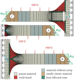
FIG. 2 FE-MESHES FOR TYPE 1 (A), TYPE 2 (B) AND

TYPE 3 (C) WELDMENTS WITH LOADINGS

Finite element models

The FE-meshes for the 2D symmetric models of type 1, 2 and 3 weldments are shown in Fig. 2 assuming plane strain con-ditions. Each of the FE-meshes includes 5 separate areas with different material properties: 1) parent material, 2) HAZ, 3) weld metal, 4) material without creep, 5) totally elastic material. In-troduction of 2 additional material types (material without creep and totally elastic material) representing reduced sets of parent material properties in the location of bending moment applica-tion avoids excessive stress concentraapplica-tions. Both FE-models use ABAQUS element type CPE8R: 8-node biquadratic plane strain quadrilaterals with reduced integration. The FE-meshes for type 1 and type 2 welds consist of 723 and 977 elements respectively. The FE-mesh for type 3 weldwent contains the range of elements from 1008 for Conf. 1 to 908 for Conf. 7 respectively.

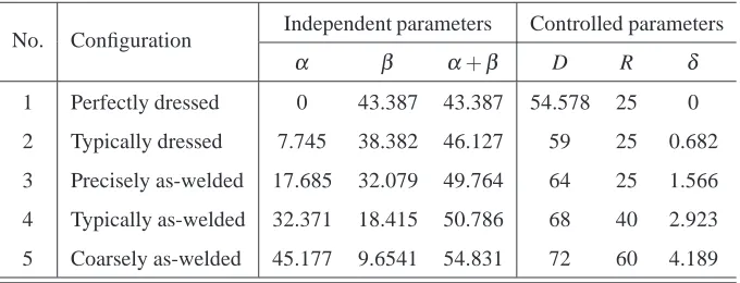
TABLE 1 GEOMETRICAL CONFIGURATIONS OF WELD PROFILES FOR TYPE 1 AND 2 WELDMENTS

No. Configuration Independent parameters Controlled parameters

α β α+β D R δ

1 Perfectly dressed 0 43.387 43.387 54.578 25 0

2 Typically dressed 7.745 38.382 46.127 59 25 0.682

3 Precisely as-welded 17.685 32.079 49.764 64 25 1.566

4 Typically as-welded 32.371 18.415 50.786 68 40 2.923

5 Coarsely as-welded 45.177 9.6541 54.831 72 60 4.189

Another effective analysis technique, successfully employed in [3], was to apply the bending moment M through the linear distribution of normal pressure P over the section of the plate as illustrated in Fig. 2 with the area moment of inertia in regard to horizontal axis X :

IX=w thk3/12, (8)

where the width of plate w = 200 mm and the thickness of plate thk = 26 mm. Therefore, the normal pressure is expressed in terms of applied bending moment M and vertical coordinate y of plate section assuming the coordinate origin in the mid-surface:

P(y) =M y/IX. (9)

STRUCTURAL INTEGRITY ASSESSMENTS Numerical creep-fatigue evaluation

Since the principal goal of the research is the formulation of parametric relations able to describe long-term structural in-tegrity of weldments, the creep-fatigue strength of the 5 config-urations from Table 1 for type 1 and 2 weldments and 7 con-figurations with differentρ values for type 3 weldments should be evaluated in a wide range of loading conditions. These con-ditions are presented by different combinations of ∆εtot in the parent plate outer fibre, as a characteristic of fatigue effects, and duration∆t of dwell period, as a characteristic of creep effects. The set of 5 values for ∆εtot is the same as in the experimen-tal studies [5, 6]. The set of ∆t values used are the same as in the previous simulation study [3]: 0, 0.5, 1, 2, 5, 10, 100, 1000 and 10000 hours. Therefore, for each of configuration 45 creep-fatigue evaluations must be performed with different values of ∆εtotand∆t. In order to estimate all values of number of cycles to failure N?, hundreds FE-simulations of the parametric models shown in Fig. 2 have been carried out, using the LMM method, material models and constants given in [3].

The concept of the proposed creep-fatigue evaluation pro-cedure, considering time fraction rule for creep-damage assess-ment, is explained in detail in [3] and consists of 5 steps:

1. Estimation of saturated hysteresis loop using the LMM; 2. Estimation of fatigue damage using S-N diagrams; 3. Assessment of stress relaxation with elastic follow-up; 4. Estimation of creep damage using creep rupture curves; 5. Estimation of total damage using an interaction diagram.

Since the LMM requires lower computational effort com-pared to other methods, it appears to be an effective tool for ex-press analysis of a large number of different loading cases us-ing automation techniques. In order to perform hundreds FE-simulations in CAE-system ABAQUS and effectively retrieve corresponding values of N?, 3 analysis improvements using au-tomation have been developed and in these parametric studies.

The first automation technique is the embedding of all 5 steps of the proposed creep-fatigue evaluation procedure in FOR-TRAN code of user material subroutine UMAT containing the implementation of the LMM and material models described in [3]. The most important parameters (derived in the 1st step of the procedure) for further creep-fatigue evaluation are the total strain range∆εtot, stressσ1at the beginning of dwell period and the elastic follow-up factor Z. These parameters from each inte-gration point with material properties for elasticity, fatigue and creep, defined in the ABAQUS input file, are transferred into a new subroutine. This subroutine implements the next 4 steps of the procedure [3], which calculates and outputs the following parameters into ABAQUS result ODB-file: time to creep rupture t∗, creep damage accumulated per cycleωcr

1c, number of cycles to fatigue failure N∗, fatigue damage accumulated per 1 cycleω_1cf, and the most important – total number of cycles to creep-fatigue failure N?based upon a damage interaction diagram.

corre-1 10 100 1000 10000 100000 1000000

1 10 100 1000 10000 100000 1000000

Non-conservative

Conservative

Number of cycles to failure N?with the LMM

N

? w

it

h

an

al

y

ti

c

fu

n

ct

io

n

optimal match

factor of 2 conf. 1 (α=0◦) conf. 2 (α=7.75◦) conf. 3 (α=17.68◦) conf. 4 (α=32.37◦)

conf. 5 (α=45.18◦)

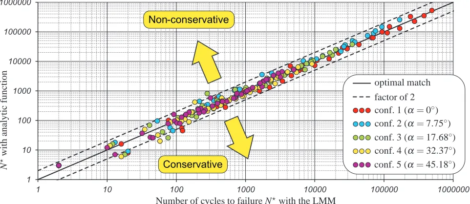
FIG. 3 COMPARISON OF N?OBTAINED WITH THE LMM AND THE ANALYTIC FUNCTION (10) FOR TYPE 1 WELDMENT

sponding to the loading case of∆εtot=1% and∆t=5 hours is presented in [11] and illustrated there in Fig. 5. Those results cor-respond to the FEA contour plots of the LMM outputs (obtained in Step 1) including∆εtot,εcr,ε_vMeq at the beginning of dwell and

εeq

vMat the end of dwell, explained in [3] and illustrated there in Fig. 9. The critical location with N?=279 cycles to failure for this case is the corner element in the weld toe adjacent to HAZ. Exactly the same approach is used to demonstrate an example of a type 1 weldment comprising geometry configuration no. 2 (typ-ically dressed) and loading case of∆εtot=1% and∆t=5 hours. Figure 6 in [11] shows the outputs of FEA with the LMM, while Fig. 7 in [11] shows the outputs of the creep-fatigue evaluation procedure. The critical location with N?=206 cycles to failure for type 1 is the same as for the type 2 weldment – the corner element in the weld toe adjacent to HAZ. The examples of FEA results for type 3 weldment under the same loading conditions and their analysis are to be presented at the conference.

The second automation technique is the development of a stand-alone application using Embarcadero Delphi integrated de-velopment environment using Delphi programming language. This simple application automatically carries out the sequence of all FE-simulations with different M (corresponding to 5∆εtot values) and∆t values for each of the configurations of type 1, 2 and 3 weldments. This is implemented by automated modi-fication of the UMAT subroutine including changing of loading values (M and∆t) and output file names, therefore producing in-dividual ABAQUS result ODB-file for each loading case.

The third automation technique is the development of a script using ABAQUS Python Development Environment (Abaqus PDE) using Python programming language [12]. This

simple script, when started in ABAQUS/CAE environment, ap-pends the list of available ABAQUS result ODB-files corre-sponding to one configuration. For each of ODB-files, it reads the values of N?in each integration point, selects the integration point with minimum value of N?over the FE-model, and writes the element number, integration point number and material name to an output text file. Therefore, the critical locations and corre-sponding values of N?are extracted automatically for all config-urations and loading cases. Obtained results can be used for the formulation of an analytic assessment model suitable for the fast estimation of N?for a variety of loading conditions ( ˜M and∆t) and geometrical weld profile parameters (α,β andρ).

Analytic assessment model

For each of the configurations for type 1, 2 and 3 weld-ments, the array of assessment results consisting of N?values corresponding to particular values of ˜M and∆t is fitted using the least squares method by the following function proposed in the form of power-law in [3]:

log(N?) =M˜−b(∆t)/a(∆t), (10)

where the fitting parameters dependent on dwell period∆t are

a(∆t) =a3log(∆t+1)3+a2log(∆t+1)2 +a1log(∆t+1) +a0 and

b(∆t) =b3log(∆t+1)3+b2log(∆t+1)2 +b1log(∆t+1) +b0,

and the independent fitting parameters (a0- a3and b0- b3) have particular values individual for each type of weldment (1, 2 and 3) and each available configuration.

In order to capture all configurations with an unified set of fitting parameters, parameters a0, a1, a2, a3, b0, b1, b2, b3should be defined as dependent on geometric parametersα, β andρ using the least squares method. For the type 1 weldments these parameters are dependent on angleαonly:

aT1

0 (α) =−4.175·10−5α2+2.72·10−3α+0.227,

aT1₁ (α) =−2.169·10−3α+1.21·10−1,

aT1₂ (α) =1.907·10−3α−7.093·10−2,

aT1₃ (α) =−5.352·10−4α+1.968·10−2,

bT1₀ (α) =−4.76324·10−3α+0.793,

bT1₁ (α) =1.42·10−4α2−8.547·10−3α+0.4028,

bT1₂ (α) =1.531·10−3α−0.3015,

bT1₃ (α) =−3.08·10−4α+8.364·10−2.

(12)

For the type 2 weldments these parameters include the de-pendence on angleα from Eqs (12) and an additional effect of angleβ as in the following form:

aT2₀ (α,β) =aT1₀ (α) +3.179·10−4β+2.355·10−3,

aT2₁ (α,β) =aT1₁ (α)−1.636·10−3β+3.043·10−2,

aT2₂ (α,β) =aT1₂ (α) +1.636·10−3β−3.043·10−2,

aT2₃ (α,β) =aT1₃ (α)−4.136·10−4β+7.33·10−3,

bT2₀ (α,β) =bT1₀ (α) +0.0291

−1.684·10−4exp(0.1622β), bT2₁ (α,β) =bT1₁ (α)−0.1789,

bT2₂ (α,β) =bT1₂ (α) +0.1558,

bT2₃ (α,β) =bT1₃ (α)−4.546·10−2.

(13)

For the type 3 weldments these parameters are dependent on ratioρonly in the following form:

aT3₀ (ρ) =−4.506·10−2ln(ρ+1) +0.285,

aT3₁ (ρ) =4.1·10−2ln(ρ+1) +4.701·10−2,

aT3₂ (ρ) =−3.202·10−2ln(ρ+1)−7.575·10−3,

aT3₃ (ρ) =8.74·10−3ln(ρ+1) +2.10773·10−3

bT3₀ (ρ) =0.118 ln(ρ+1) +0.57,

bT3₁ (ρ) =8.742·10−2ln(ρ+1) +0.195,

bT3₂ (ρ) =−7.197·10−2ln(ρ+1)−0.152,

bT3₃ (ρ) =1.397·10−2ln(ρ+1) +4.034·10−2.

(14)

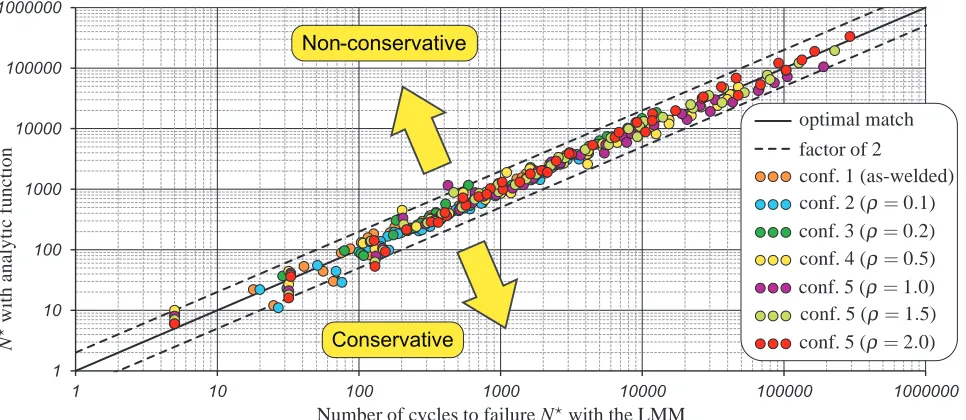
The verification of the fit quality using the the geometrical parameters (α,β andρ) for the proposed relations (12) - (14)

is implemented by applying Eqs (10) and (11) to estimate N?. Number of cycles to failure N?is estimated for all configurations using the corresponding values of angles (αandβ) from Table 1 and ratioρ (2.0, 1.5, 1.0, 0.5, 0.2, 0.1 and→0). The compari-son is done for the same load combinations as were used for the LMM analyses. The results of the verification are illustrated on diagrams in Fig. 3 for type 1, Fig. 4 for type 2 and Fig. 5 for type 3 weldments in the form of N? obtained with the analytic function (10) vs. N?obtained with the LMM. Comparison of the analytic and numeric N?for all types of weldments shows that the quality of analytic predictions is quite close to the line of op-timal match and provides a uniform scatter of results through all variants of loading conditions and configurations. The discrep-ancy between analytic predictions and numerical LMM outputs is generally found to be within the boundaries of an inaccuracy factor equal to 2, which is allowable for engineering analysis, producing both conservative and non-conservative results.

Having defined the number of cycles to failure N? by Eq. (10), the residual service life in years is therefore dependent on the duration of 1 cycle, which consists of dwell period∆t and relatively short time of deformation as follows:

L?=N? ∆t

365·24+

2∆εtot(M˜) ˙

ε(365·24·60·60)

, (15)

where ˙ε =0.03%/s is a strain rate according to experimen-tal conditions [5, 6], and the parametric analytical relations for ∆εtot(M˜) are derived in Sect. 3 of [11]. These relations for

∆εtot(M˜) include the geometrical parameters of parent plate cross-section (thk and w) and weld profile (α, β andρ), and parent plate material parameters (E,ν, B,β,σy).

PARAMETRIC FORMULATION OF FSRF

Since the function N?(_M,˜ _{∆t)proved its validity in the} previ-ous subsection, it can be applied for the fast creep-fatigue assess-ments of new welded structures during the design stage. How-ever, it is generally hard to generate conclusions about the ser-vice conditions(_M,˜ _{∆t)required to estimate particular value of} N?. Loading conditions comprise a wide range of mechanical loading described by ˜M or corresponding range of∆εtotin par-ent material adjacpar-ent to welded joints. Thus, introduction of a Fatigue Strength Reduction Factor (FSRF) allows a wide range of mechanical loading relevant to application area of a designed welded structure to be captured. The FSRF takes into account the difference in behaviour of the weldment compared to the par-ent material, considering weldmpar-ents to be composed of parpar-ent material. The FSRF is determined experimentally by comparing the fatigue failure data of the welded specimen with the fatigue curve derived from tests on the parent plate material.

1 10 100 1000 10000 100000 1000000

1 10 100 1000 10000 100000 1000000

Non-conservative

Conservative

Number of cycles to failure N?with the LMM

N

? w

it

h

an

al

y

ti

c

fu

n

ct

io

n

optimal match

factor of 2

conf. 1 (α=0◦,β =43.39◦) conf. 2 (α=7.75◦,β =38.38◦) conf. 3 (α=17.68◦,β=32.08◦) conf. 4 (α=32.37◦,β=18.42◦) conf. 5 (α=45.18◦,β =9.65◦)

FIG. 4 COMPARISON OF N?OBTAINED WITH THE LMM AND THE ANALYTIC FUNCTION (10) FOR TYPE 2 WELDMENT

1 10 100 1000 10000 100000 1000000

1 10 100 1000 10000 100000 1000000

Non-conservative

Conservative

Number of cycles to failure N?with the LMM

N

? w

it

h

an

al

y

ti

c

fu

n

ct

io

n

optimal match

factor of 2

conf. 1 (as-welded) conf. 2 (ρ=0.1) conf. 3 (ρ=0.2) conf. 4 (ρ=0.5)

conf. 5 (ρ=1.0) conf. 5 (ρ=1.5) conf. 5 (ρ=2.0)

FIG. 5 COMPARISON OF N?OBTAINED WITH THE LMM AND THE ANALYTIC FUNCTION (10) FOR TYPE 3 WELDMENT

weldments taking into account dressed and as-welded variants, which consider only the reduction of fatigue strength of ments compared to the parent material. For austenitic steel weld-ments [13], FSRF = 1.5 is prescribed for both variants of type 1, FSRF = 1.5 for type 2 dressed and FSRF = 2.5 for as-welded variant, and FSRF = 3.2 is prescribed for both variants of type 3. All this variety of the FSRFs is representative of the reduction in fatigue endurance caused by the local strain rangeεtot enhance-ment in the weldenhance-ment region due to the material discontinuity and geometric strain concentration effects. The introduction of

FSRF as dependent on∆t in [3] using function N?(_M,˜ _{∆t)for the} case of type 2 dressed weldment allowed the influence of creep to be taken into account, and to provide the adjusted values of FSRF for creep-fatigue operation conditions. Therefore, the same ap-proach [3] is applied to obtain∆t-dependent FSRFs for a variety of geometrical configurations considering additional dependence on parameters of weld profile (α,β andρ).

11

10

9

8

7

6

5

4

3

2

1

0.01 0.1 1 10 100 1000 10000

dwell time (hours)

F

S

R

F

Configurations: 1. Perfectly dressed 2. Typically dressed 3. Precisely as-welded 4. Typically as-welded 5. Coarsely as-welded

FIG. 6 FSRFS DEPENDENT ON DWELL PERIOD∆t FOR

DIFFERENT CONFIGURATIONS OF TYPE 1 WELDMENTS

0.01 0.1 1 10 100 1000 10000 11

10

9

8

7

6

5

4

3

2

1

dwell time (hours)

F

S

R

F

Configurations:

1. Perfectly dressed 2. Typically dressed 3. Precisely as-welded 4. Typically as-welded 5. Coarsely as-welded

FIG. 7 FSRFS DEPENDENT ON DWELL PERIOD∆t FOR

DIFFERENT CONFIGURATIONS OF TYPE 2 WELDMENTS

11

10

9

8

7

6

5

4

3

2

1

0.01 0.1 1 10 100 1000 10000

dwell time (hours)

F

S

R

F

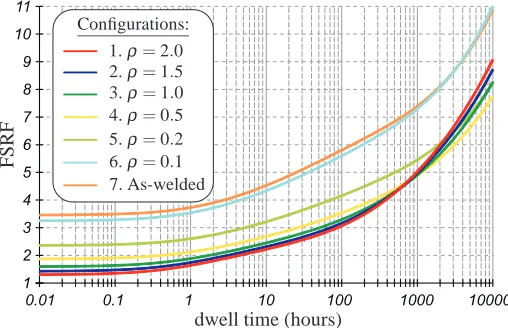
Configurations:

1.ρ=2.0

2.ρ=1.5

3.ρ=1.0

4.ρ=0.5

5.ρ=0.2

6.ρ=0.1

7. As-welded

FIG. 8 FSRFS DEPENDENT ON DWELL PERIOD∆t FOR

DIFFERENT CONFIGURATIONS OF TYPE 3 WELDMENTS

TABLE 2 THE VALUES OF FSRFS FOR PURE FATIGUE

FOR TYPES 1, 2 AND 3 WELDMENTS FROM FIGS 6–8

Conf. 1 2 3 4 5 6 7

Type 1 1.146 1.444 2.062 2.896 3.308 — —

Type 2 1.362 1.682 2.372 3.137 3.430 — —

Type 3 1.302 1.425 1.595 1.872 2.362 3.252 3.459

∆εtot(N?,∆t,[α,βorρ]). This relation describes the∆εtotin the parent material remote from weldment corresponding to particu-lar values of N?and∆t for a particular geometrical configuration of weldment defined byα,βorρ. Thus, the FSRFs, appropriate to varying values of∆t and equal values of N?, are defined by the relation between the S–N diagram corresponding to fatigue fail-ures of parent material plate and S–N diagrams for a weldment:

FSRF=∆εtotpar(N?)/∆εtot(N?,∆t,[α,βorρ]), (16)

where the S–N diagram for parent material plate is defined as

log ∆ε_totpar

=p0+p1log(N∗) +p2log(N∗)2, (17)

with the following polynomial coefficients referring to [13]: p0=2.2274, p1=−0.94691 and p2=0.085943.

The FSRFs estimated by Eq. (16) corresponding to the range of∆t∈

0...105 hours are defined in some particular range of N?. This range is different for each value of∆t characterised by reducing value of the average N? with the growth of ∆t. The upper bound of the N? range is governed by the mathematical upper limit of the S–N diagram∆ε_totpar(N?) for parent material plate, which is defined in [3] as log(N_max? ) =p1/(2 p2) =5.51 or∆ε_totpar(105.51_{) =0.416%. The lower bound of the N}?_{range is} flexible and governed by∆t using the following function:

log(N_min? ) =3−0.5 log(∆t+1). (18)

The FSRF for type 1 dressed weldments is within the range 1.146–1.444 depending on the quality of grinding, while R5 gives the value 1.5 (refer to [13]), which is more conservative. The FSRF for type 1 precisely welded joints without grind-ing is within the range 1.444–2.062 dependgrind-ing on the quality of welding, while R5 gives the same value 1.5, which is non-conservative. The FSRF for type 1 coarsely welded joints with-out any additional treatment may reach up to 3.308, while R5 doesn’t give any value for this case.

The FSRF for type 2 dressed weldments is within the range 1.362–1.682 depending on the quality of grinding, while R5 gives the value 1.5, which approximately corresponds to aver-age value for the obtained range. The FSRF for type 2 precisely welded joints without grinding is within the range 1.682–2.372 depending on the quality of welding, while R5 gives the value 2.5, which is more conservative. The FSRF for type 2 coarsely welded joints without any additional treatment may reach up to 3.43, while R5 doesn’t give any value for this case.

The FSRF for type 3 dressed weldments is within the range 1.302–1.425, for type 3 welded joints with moderate TIG dress-ing it is within the range 1.425–2.362 dependdress-ing on the amount of TIG dressing, while R5 also doesn’t give any value for these cases. The FSRF for type 3 as-welded joints without any addi-tional treatment may reach up to 3.252–3.459, while R5 gives the value 3.2, which approximately corresponds to lower bound for the obtained range. It should be noted that the value of FSRF for type 3 recommended by R5 procedure may be significantly conservative, if some kind of TIG dressing is applied.

CONCLUSIONS

The parametric study on creep-fatigue strength of the steel AISI type 316N(L) weldments of types 1, 2 and 3 according to classification of R5 Vol. 2/3 procedure [7] at 550◦C has been implemented using the LMM. The study is based upon the lat-est developed creep-fatigue evaluation procedure [3] consider-ing time fraction rule for creep-damage assessment. Proposed approach improves upon existing design techniques, e.g. in R5 procedure [7], by considering the significant influence of creep. Moreover, the obtained FSRFs for pure fatigue revises the val-ues recommended in R5 Procedure [7] removing the redundant conservatism for type 1 and 3 dressed weldments and type 2 un-dressed weldments.

ACKNOWLEDGMENT

The authors deeply appreciate the Engineering and Physical Sciences Research Council (EPSRC) of the UK for the financial support in the frames of research grant no. EP/G038880/1, the University of Strathclyde for hosting during the course of this work, and EDF Energy for the experimental data.

REFERENCES

[1] Lee, Y.-L., Barkey, M. E., and Kang, H.-T., 2012. Metal Fatigue Analysis Handbook: Practical Problem-Solving Techniques for Computer-Aided Engineering. Butterworth-Heinemann, Oxford.

[2] Radaj, D., Sonsino, C. M., and Fricke, W., 2006. Fatigue Assessment of Welded Joints by Local Approaches, 2nd ed. Woodhead Publishing Limited, Cambridge.

[3] Gorash, Y., and Chen, H., 2013. “Creep-fatigue life as-sessment of cruciform weldments using the linear match-ing method”. Int. J. of Pressure Vessels & Pipmatch-ing. in press, DOI: 10.1016/j.ijpvp.2012.12.003.

[4] Chen, H. F., Chen, W., and Ure, J., 2012. “Linear matching method on the evaluation of cyclic behaviour with creep effect”. In Proc. ASME Pressure Vessels & Piping Conf. (PVP2012), ASME. July 15-19.

[5] Bretherton, I., and Budden, P. J., 1999. “Assessment of creep-fatigue endurance of large cruciform weldments”. In Trans. 15th Int. Conf. on Structural Mechanics in Reactor Technology, no. SMiRT15 – F05/2. IASMiRT, Seoul, Ko-rea, pp. 185–192.

[6] Bretherton, I., Knowles, G., Hayes, J.-P., Bate, S. K., and Austin, C. J., 2004. PC/AGR/5087: Final report on the fatigue and creep-fatigue behaviour of welded cruci-form joints. Report for British Energy Generation Ltd no. RJCB/RD01186/R01, Serco Assurance, Warrington, UK. [7] Ainsworth, R. A., ed., 2003. R5: An Assessment Procedure

for the High Temperature Response of Structures. Proce-dure R5: Issue 3. British Energy Generation Ltd, Glouces-ter, UK.

[8] British Standard, 2010. Welding - Basic welded joint details in steel - Part 1: Pressurized components. No. EN 1708-1:2010. London, UK.

[9] British Standard, 2007. Welding - Fusion-welded joints in steel, nickel, titanium and their alloys - Quality levels for imperfections. No. EN ISO 5817:2007. London, UK. [10] Pedersen, M. M., Mouritsen, O. O., Hansen, M. R.,

An-dersen, J. G., and Wenderby, J., 2010. “Comparison of post weld treatment of high strength steel welded joints in medium cycle fatigue”. Welding in the World, 54(7-8), pp. R208–R217.

[11] Gorash, Y., and Chen, H., 2013. “A parametric study on creep-fatigue strength of welded joints using the lin-ear matching method”. Int. J. of Fatigue. submitted, no. IJFATIGUE-D-13-00028, StrathPrints URI.

[12] DASSAULT SYSTEMES` SIMULIA CORP., 2010. ABAQUS Scripting User’s Manual, Version 6.10 ed.