On the adaptive selection of the parameter in stabilized finite element approximations

(1)

SIAM J. NUMER.ANAL. c 2013 Society for Industrial and Applied Mathematics Vol. 51, No. 3, pp. 1585–1609

ON THE ADAPTIVE SELECTION OF THE PARAMETER IN

STABILIZED FINITE ELEMENT APPROXIMATIONS

∗

MARK AINSWORTH†, ALEJANDRO ALLENDES‡, GABRIEL R. BARRENECHEA§, AND

RICHARD RANKIN¶

Abstract. A systematic approach is developed for the selection of the stabilization parameter for stabilized finite element approximation of the Stokes problem, whereby the parameter is chosen to minimize a computable upper bound for the error in the approximation. The approach is ap-plied in the context of both a single fixed mesh and an adaptive mesh refinement procedure. The optimization is carried out by a derivative-free optimization algorithm and is based on minimizing a new fully computable error estimator. Numerical results are presented illustrating the theory and the performance of the estimator, together with the optimization algorithm.

Key words.stabilized ﬁnite element method, stabilization parameter, computable error bounds, derivative-free optimization

AMS subject classifications.65N15, 65N30

DOI.10.1137/110837796

1. Introduction.

The numerical approximation of the Stokes problem

gener-ally follows one of two complementary approaches. The ﬁrst consists of using discrete

velocity-pressure spaces satisfying the discrete inf-sup condition. Many such methods

are available in the literature (see [20, 10] for extensive reviews). However, one

per-ceived drawback of this approach is the fact that the discrete spaces cannot be of the

same polynomial order in both variables while maintaining stability. The second

ap-proach consists of adding so-called stabilizing terms to the discrete formulation using

an equal (or the lowest unequal) order velocity-pressure combination. These

stabiliz-ing terms can depend on residuals of the equation at the element level or can simply

be based on compensating for the inf-sup deﬁciency of the pressure. For extensive

reviews on diﬀerent alternatives for stabilized ﬁnite element methods, see [6, 30].

One characteristic feature of stabilized methods is the presence of a positive

con-stant multiplying the stabilization term. Naturally, the question of the selection of

the actual value of the stabilization parameter in practical computation arises, which,

although not aﬀecting the rate of convergence, can have a signiﬁcant impact on the

absolute value of the error. Considerable eﬀort has been expended in the quest to

avoid having to make an ad hoc decision about the speciﬁc choice of the parameter.

∗_{Received by the editors June 17, 2011; accepted for publication (in revised form) March 20,}

2013; published electronically May 28, 2013. The ﬁrst and fourth authors were supported by the Engineering and Physical Sciences Research Council of Great Britain under the Numerical Algorithms and Intelligent Software (NAIS) for the evolving HPC platform grant EP/G036136/1.

http://www.siam.org/journals/sinum/51-3/83779.html

†_{Division of Applied Mathematics, Brown University, Providence, RI 02912 (mark ainsworth@}

brown.edu).

‡_{Departamento de Matem´}_{atica, Universidad T´}_{ecnica Federico Santa Mar´ıa, Casilla 110-V,}

Val-para´ıso, Chile ([email protected]). This author was supported by the Faculty of Science of Strathclyde University and Comisión Nacional de Investigación Cient´ıfica y Tecnológica – CONICYT (Chile) through a research studentship and grant 79090008, Fortalecimiento del grupo de Análisis y Modelamiento Matemático, Valpara´ıso.

§_{Department of Mathematics and Statistics, University of Strathclyde, Glasgow G1 1XH, Scotland}

([email protected]).

¶_{Computational and Applied Mathematics Department, Rice University, Houston, TX 77005}

([email protected]).

1585

(2)

Variational multiscale methods (including residual-free bubbles and, recently, Petrov

Galerkin Enriched methods [22, 11, 4, 5, 3]) may be regarded as a systematic approach

to the selection of an explicit, closed form of the value of the stabilization parameter,

thereby rendering the methods parameter-free.

In this work our approach is based on the premise that the best parameter is the

one for which the error is minimal. Of course, the true value of the error is generally

unknown. However, if a computable quantity

η(α) is available, which depends on

the value

α

of the stabilization parameter, and for which a two-sided bound on the

true error in an appropriate norm

|||

(

e

_V

, e

_P

)

|||

holds, i.e., there exists a constant

c >

0 independent of

α, for which

(1.1)

c η(α)

≤ |||

(

e

_V

, e

_P

)

||| ≤

η(α),

then we may, in lieu of minimizing the true error, seek the value of

α

which minimizes

the value of

η(α). This approach constitutes an objective, rational approach to the

selection of the stabilization parameter. Of course, the quality of the results will

reﬂect the quality of the bounds (1.1): If

c

= 1, then we would be minimizing the

true error, but this is, of course, unrealistic. In any case, what is really needed is

for the value of

α

at which

η(α) has a minimum to coincide with the value of

α

at

which the true error has a minimum. The development of a method for deﬁning a

computable quantity

η(α), satisfying (1.1) up to higher-order oscillation terms, is a

key component of our approach and occupies section 5. As a fringe beneﬁt, we obtain

an expression for

η(α) which enables us to estimate the error for virtually any existing

stabilized method for the Stokes problem.

The search for the optimal value of the stabilization parameter has been

consid-ered before. For example, in [8] a residual based a posteriori error estimator was also

minimized in order to obtain a value for the stabilization parameter (see also [25] for

convection-diﬀusion problems), while in [31] the value is chosen by minimizing the

condition number of the associated Schur complement system for the pressure ﬁeld.

The development of the measure

η(α) is only one part of the story and we must

also select an algorithm for approximating its minima. The expression for

η(α)

de-pends on the stabilized ﬁnite element approximation obtained using a particular value

α

for the stabilization parameter. Thus, each evaluation of

η(α) entails the

compu-tation of a ﬁnite element approximation.

Furthermore, one does not have ready

access to derivative information. These considerations suggest the use of a

derivative-free optimization (DFO) approach to search for the value

α

_opt

for which

η(α) is

minimized.

Numerical examples are presented showing the performance of the approach in

the case of a ﬁxed mesh for a variety of stabilized ﬁnite element methods. The results

indicate that the algorithm does indeed enable us to select a near-optimal value of the

stabilization parameter. The approach is then applied to the case of ﬁnite element

approximation on a sequence of adaptively reﬁned meshes, again yielding satisfactory

results.

We summarize the main features of the work:

• the construction of a fully computable a posteriori error bound which is robust

with respect to the stabilization parameter and which is applicable to a wide

range of stabilized ﬁnite element methods;

• the selection of the value of the stabilization parameter based on

minimiz-ing the a posteriori error bound; and

• the combination of this approach with an adaptive reﬁnement procedure.

(3)

ADAPTIVE SELECTION OF THE STABILIZATION PARAMETER

1587

The paper is organized as follows. In the next section we give some preliminaries

that will be needed throughout the manuscript along with a description of the diﬀerent

stabilized ﬁnite element methods considered. Sections 3 and 4 are devoted to the

optimization procedure, the summary of the main results of the a posteriori analysis,

and numerical examples. Finally, the technical proofs related to the a posteriori error

estimate are given in section 5, and conclusions are drawn in section 6.

2. Preliminaries.

For a bounded open domain,

G

⊂

R

d

_{, where}

_d

_{= 1,}

_2;

_L

2

_(G)

denotes the space of square integrable functions over

G,

L

2₀

(G) represents functions

belonging to

L

2

(G) with zero average in

G,

H

1

(G) is the usual Sobolev space, and

H

₀1

(G) denotes the subspace of

H

1

(G) consisting of functions whose trace is zero on

the boundary of

G. Let (

· ,

· )

_G

denote the inner product in

L

2

(G) (or in

L

2

(G)

2

,

L

2

(G)

2×2

when necessary). The norm of the space

H

m

_{(G) is denoted by}

_·

m,G

,

with the convention that when

m

= 0 we have that

·

₀_,G

=

·

_L2₍_G₎

. We use

bold letters to denote the vector-valued counterparts of the Sobolev and Lebesgue

spaces, e.g.,

H

1₀

(G) =

H

₀1

(G)

×

H

₀1

(G), and use an extra underaccent to denote their

matrix-valued counterparts, e.g.,

≈

L

2

_{(G) =}

_L

2

_(G)

2×2

_.

Let Ω

⊂

R

2

be an open polygonal domain with boundary Γ. Let

{P}

be a family

of partitions of Ω, where each partition is built up using shape regular triangles

K

such that Ω =

_K_∈P

K

and the nonempty intersection of two distinct elements is

either a single common edge or vertex of both elements.

2.1. Notation.

For convenience, we shall summarize all the notation used

through-out the manuscript related to the partition of the domain.

For a ﬁxed partition

P

let

• E

denote the set of all edges;

• E

I

⊂ E

denote the set of interior edges;

• E

Γ

⊂ E

denote the set of boundary edges;

• V

denote the set

{

x

_n

}

of all element vertices;

• Ω

_n

=

{

K

∈ P

:

x

_n

∈

K

for a ﬁxed

x

_n

∈ V}

;

• E

n

=

{

γ

∈ E

:

x

n

∈

γ

for a ﬁxed

x

n

∈ V}

;

• λ

_n

denote the usual barycentric coordinate associated to the vertex

x

_n

∈ V

and let

λ

(_n1)

=

λ

_n

0

T

and

λ

(_n2)

=

0 λ

_n

T

.

For an element

K

∈ P

let

• Pn

(K) denote the space of polynomials on

K

of total degree at most

n;

• E

K

denote the set containing the individual edges of the element;

• _Ω

˜

K

=

{

K

∈ P

:

K

∩

K

=

∅}

;

• Ω

_K

=

{

K

∈ P

:

E

_K

∩ E

_K

=

∅}

;

• |

K

|

denote the area of

K;

• v

_K

=

_|1 K|

K

v d

x

denote the mean value of

v

on the element

K;

• h

_K

denote the diameter of

K;

• n

ˆ

K

γ

denote the unit exterior normal vector to edge

γ

∈ E

K

.

For an edge

γ

∈ E

let

• Pn

(γ) denote the space of polynomials on

γ

of total degree at most

n;

• V

γ

=

{

x

n

∈ V

:

x

n

∈

γ

}

denote the set of endpoints of an edge

γ;

• |

γ

|

denote the length of

γ.

We also deﬁne the projection operator Π

_K

:

L

2

(K)

→

P

₁

(K)

2

by

(2.1)

(

t

−

Π

_K

t

,

θ

)

_K

= 0

∀

θ

∈

P

₁

(K)

2

.

(4)

2.2. Model problem.

We are interested in the following Stokes problem: For

given data

f

∈

L

2

(Ω), ﬁnd a velocity

u

and a pressure ﬁeld

p

such that

u

=

0 on Γ

and

(2.2)

−

νΔ

u

+

∇

p

=

f

and

∇ ·

u

= 0

in Ω

,

where

ν >

0 is the ﬂuid viscosity. The weak formulation of the Stokes problem then

reads as follows: Find (

u

, p)

∈

H

1₀

(Ω)

×

L

2₀

(Ω) such that

(2.3)

A

(

u

, p;

v

, q) =

F

(

v

)

for all (

v

, q)

∈

H

1₀

(Ω)

×

L

2₀

(Ω),

where

(2.4)

A

(

u

, p;

v

, q) =

ν(

∇

u

,

∇

v

)

_Ω

−

(p,

∇

· v

)

_Ω

+ (q,

∇

· u

)

_Ω

and

F

(

v

) = (

f

,

v

)

_Ω

.

The well-posedness of problem (2.3) is a consequence of two facts: the bilinear

form

ν(

∇

u

,

∇

v

)

_Ω

is coercive on

H

1₀

(Ω) owing to Poincar´

e’s inequality and hence is

also coercive on the subspace

(2.5)

X

=

v

∈

H

1₀

(Ω) :

∇

· v

= 0

,

and there exists a constant

β >

0 such that

(2.6)

sup

v∈H1 0(Ω)\{0}

(q,

∇

· v

)

_Ω

∇

v

0,Ω

≥

β

q

₀_,_Ω

∀

q

∈

L

2₀

(Ω).

The constant

β

is known as the inf-sup constant for the domain Ω. For more details

concerning the well-posedness of problem (2.3), see [20].

2.3. Stabilized finite element methods.

For nonnegative integers

m, let

X

_hm

=

v

∈

L

2

(Ω) :

v

_|_K

∈

Pm

(K)

∀

K

∈ P

and

X

m_h

= (X

m h

)

2

_{. Let}

_V

h

=

X

1h

∩

H

10

(Ω) and let

Q

h

⊂

X

_h1

∩

L

20

(Ω). A stabilized

ﬁnite element approximation of the Stokes problem then reads as follows: Find a pair

(

u

_h

, p

_h

)

∈

V

_h

×

Q

_h

such that

(2.7)

A

(

u

_h

, p

_h

;

v

, q) +

α

S

(

u

_h

, p

_h

,

f

;

q) =

F

(

v

, q)

∀

(

v

, q)

∈

V

_h

×

Q

_h

,

where

S

(

u

_h

, p

_h

,

f

;

q) is the stabilization term and the parameter

α

is a positive

con-stant, sometimes referred to as the

stabilization parameter

. Often, the developers of

a particular stabilized method give a recommendation

α

_rec

for the value of the

sta-bilization parameter to be used in practical computations, but in some cases no such

value is identiﬁed. Many stabilized ﬁnite element methods are available, and below

we give examples of stabilized ﬁnite element methods which can be used to

approx-imate the solution of the Stokes problem. We shall employ various combinations of

discrete velocity-pressure spaces, depending on the particular choice of stabilization

(see Table 1).

• Galerkin least-squares type methods (GLS) [24, 30, 23, 19, 26]: The stabilizing

term is given by

S

(

u

_h

, p

_h

,

f

;

q) =

−

K∈P

h

2_K

ν

(

f

+ Δ

u

h

− ∇

p

h

,

∇

q)

K

+

γ∈EI

|

γ

|

ν

([[p

h

]]

γ

,

[[q]]

γ

)

γ

,

(5)

[image:5.612.151.365.123.165.2]

1589

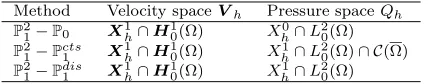
Table 1

Discrete velocity-pressure space combinations used in conjunction with the stabilized formulations.

Method Velocity spaceVh Pressure spaceQh P2

1−P0 X1h∩H01(Ω) Xh0∩L20(Ω) P2

1−Pcts1 X1h∩H01(Ω) Xh1∩L20(Ω)∩ C(Ω) P2

1−Pdis1 X1h∩H10(Ω) Xh1∩L20(Ω)

where [[v]]

_γ

denotes the jump of

v

across

γ, and may be used in conjunction with a

P

2

1

−

P

cts1

or a

P

21

−

P

dis1

or a

P

21

−

P

0

pair. For this type of method the stabilization

parameter is often recommended to be taken as

α

_rec

= 1/24.

• Brezzi and Pitk¨

aranta (BP) [12]: The stabilizing term reads

S

(

u

_h

, p

_h

,

f

;

q) =

K∈P

h

2_K

ν

(

∇

p

h

,

∇

q)

K

for a

P

2₁

−

P

cts

1

pair. For this method the authors do not recommend a particular

choice of

α, so in the absence of further information, we select

α

_rec

= 1.

• Polynomial pressure methods (PPS) [9, 17]: The stabilizing term reads

S

(

u

_h

, p

_h

,

f

;

q) =

K∈P

1 ν

((I

−

Ψ)p

h

,

(I

−

Ψ)q)

K

,

and the operator Ψ may be taken as (Ψv)

_|_K

=

v

_K

for the

P

2₁

−

P

cts

1

pair or a Cl´

ement-like interpolant for the

P

2₁

−

P

₀

pair. (See section 6 in [9] for more details about the

operator Ψ.) This method is recommended with a stabilization parameter

α

_rec

= 1.

methods.

All the previous methods constitute stable and convergent schemes. However,

alternative methods exist based on discretizing a regularization of the basic Stokes

problem. Such methods, while stable, are inconsistent and nonconvergent in general,

but can nevertheless deliver useful approximations if the value of the regularization

parameter

α

is judiciously selected. One example of such a method is the following:

• Penalty pressure-type methods (PEPS) [13]: The stabilizing term reads

S

(

u

_h

, p

_h

,

f

;

q) =

K∈P

(p

_h

, q)

_K

and may be used in conjunction with a

P

2₁

−

P

cts

1

or a

P

21

−

P

1dis

or a

P

21

−

P

0

pair. We

take

α

_rec

= 1.

The estimators that we obtain are valid for all the above mentioned methods.

Moreover, they remain valid in the case of nonhomogeneous Dirichlet data

u

=

u

_D

on Γ, for given

u

_D

∈

X

1_h

∩

H

1

(Ω). Furthermore, from now on,

c

and

C

will denote

positive constants which are independent of any mesh size, the viscosity

ν, and the

stabilization parameter

α.

3. An algorithm for selecting the stabilization parameter on a given

mesh.

Although the a priori rate of convergence of a stabilized method is independent

of the value of the stabilization parameter (provided the discrete problem is

well-posed), the absolute value of the error varies depending on the choice of the parameter.

In order to illustrate this point we consider two example problems.

(6)

Problem

1. We consider Ω = (0,

1)

2

(the unit square).

For this domain, a

lower bound of 0.38 for the value of the inf-sup constant

β

is proved in [32]. We

took

ν

= 1 and let

f

be such that the exact velocity and pressure are given by

u

=

[x

2

(x

−

1)

2

y(y

−

1)(2y

−

1),

−

y

2

(y

−

1)

2

x(x

−

1)(2x

−

1)] and

p

=

xy(1

−

x)(1

−

y)

−

1/36.

Problem

2. We consider the T-shaped domain Ω = ((

−

1.5,

1.5)

×

(0,

1))

∪

((

−

0.5,

0.5)

×

(

−

2,

1)). From [32] we have that 0.1 is a lower bound for the

inf-sup constant

β

for this domain. We took

ν

= 1 and let

f

=

0 and imposed Dirichlet

boundary conditions of

u

= (y,

0) on

x

=

±

1.5,

u

= (1,

0) on

y

= 1 and

u

= (0,

0)

elsewhere on the boundary.

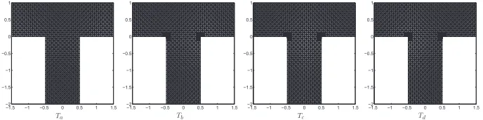
We shall present results for Problems 1 and 2 obtained using meshes

S

to

S

_d

and

T

_a

to

T

_d

shown in Figures 1 and 2, respectively.

The following norm is used to measure the velocity and the pressure errors:

|||

(

e

_V

, e

_P

)

|||

=

ν

2

∇

e

_V

₀2_,_Ω

+

β

2

e

_P

2₀_,_Ω

1/2

.

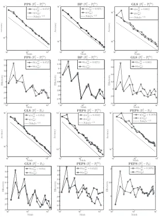
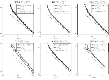
The values of norms of the errors obtained for various stabilized schemes and

various values of the stabilization parameter on ﬁxed meshes from Figures 1 and 2

are illustrated in Figures 3 and 4 for Problem 1. For Problem 2, since we do not have

at hand the analytical solution, we build a numerical reference solution and compute

the errors with respect to it. For that, we solved Problem 2 using a Taylor–Hood

discretization (

P

cts

2

−

P

cts1

) on a highly reﬁned mesh which we obtained following the

same reﬁnements as in Figure 2 (reﬁne about the reentrant corners) until we built a

mesh with 261,348 elements, and used that solution as an “exact” solution to compute

the errors with respect to. The results are depicted in Figure 5. It is clear that in some

cases the choice of the parameter

α

can signiﬁcantly aﬀect the errors. In particular,

an inappropriate choice can result in a loss of a factor of two, or sometimes much

more, in the accuracy compared with a more judicious choice. In terms of practical

computation this means that a careful choice of

α

can sometimes be at least as eﬀective

as a global mesh reﬁnement.

Fig. 1_. _{Uniform meshes}S_with ₅₁₂_,S_a _with ₂₀₄₈_,S_b_with ₄₀₉₆_{, and} S_c _with ₈₁₉₂_elements

and distorted meshS_dwith 412elements for Problem1.

Fig. 2_. _Meshes T_a _with ₂₅₆₀_, T_b _with ₅₀₇₆_, T_c _with ₇₁₀₈ _and T_d _with _11,006 _{elements for}

Problem 2.

[image:6.612.83.433.461.532.2] [image:6.612.91.435.575.661.2]

(7)

1591

Fig. 3_. _{Comparison of the estimated and true errors for diﬀerent values of}α_{using mesh}S_c

for Problem 1.

(8)

Fig. 4_. _{Comparison of the estimated and true errors for diﬀerent values of}α _{using mesh}S_d

for Problem 1.

(9)

1593

Fig. 5. Comparison of the estimated and true errors for diﬀerent values ofα using meshT_c

for Problem 2.

Ideally, we would like to select the best value of the stabilization parameter for

each problem, each mesh, and each discretization scheme. The following result, which

summarizes the ﬁndings of section 5, will be helpful in this respect.

Theorem 3.1.

Let

α >

0 and

e

_V

=

u

−

u

_h

and

e

_P

=

p

−

p

_h

denote the error

in the velocity and pressure approximations obtained using a stabilized finite element

formulation. Then,

(3.1)

ν

∇

e

_V

₀_,_Ω

≤

η

_V

(α),

β

e

_P

₀_,_Ω

≤

η

_P

(α),

and

|||

(

e

_V

, e

_P

)

||| ≤

η(α),

where the velocity and pressure error estimators are given by

(3.2)

η

_V

(α)

2

= Φ

2_c

+

ν

2

Φ

2_nc

and

η

_P

(α)

2

= (Φ

∗_c

+

ν

Φ

_nc

)

2

,

respectively, and the total error estimator is given by

(3.3)

η(α) =

η

_V

(α)

2

+

η

_P

(α)

2

1/2

,

(10)

with

Φ

_c

,

Φ

_nc

and

Φ

∗_c

, being given in

(5.21)

,

(5.22)

, and

(5.29)

, respectively. Moreover,

there exists a positive constant

c

independent of

α

,

ν

and any mesh size, such that

(3.4)

c η

_K

(α)

2

≤

K∈Ω˜K

ν

2

∇

e

_V

2₀_,K

+

β

2

e

P

02,K

+

h

2K

f

−

Π

Kf

20,K

,

where

η

_K

(α)

is given in

(4.1)

.

Proof

. The upper bounds follow from Theorems 5.2 and 5.3. The proof of (3.4)

is given in section 5.5.

It should be borne in mind that the estimator

η(α) is computed using the ﬁnite

element approximation obtained using the value

α

as the stabilization parameter.

The values of the quantities

η(α),

η

_V

(α), and

η

_P

(α) are shown along with the true

errors in Figures 3 to 5. We ﬁrst observe that both components of the error and

the estimator seem sensitive to the choice of

α

and that both components of the

estimator have a similar qualitative behavior to the individual errors. We observe

as well that the total error

|||

(

e

_V

, e

_P

)

|||

and the complete estimator

η(α) are more

in agreement than both the components, in terms of sensitivity to the choice of

α.

Signiﬁcantly, both exhibit minima at roughly the same locations. This correlation

suggests selecting the stabilization parameter

α

to minimize the upper bound

η(α)

for the true error

|||

(

e

_V

, e

_P

)

|||

. While the values of the estimated and true errors may

diﬀer, the proximity of the minimizers means that the resulting choice of

α

will be

near optimal.

It remains to select an appropriate method for obtaining the minimizer of

η(α).

We use the trust-region DFO algorithm (see [14] and references therein) to

approxi-mate the minimizer of

η(α). For the reader’s convenience, we give a brief description

of the method, which is described in full detail in [15, 16].

We begin by choosing constants

ε

_D

,

Λ,

Δ

_max

>

0, 0

≤

tol

₀

≤

tol

₁

<

1, 0

< ω

₀

<

1 < ω

₁

and a trust-region radius Δ

₀

∈

(0,

Δ

_max

]. Construct a fully quadratic model

(in the sense of section 3 in [16]) by evaluating

η(α) at a set of three sample points

α

₀

=

{

α

₁

, α

₂

, α

₃

}

to obtain a quadratic interpolant, given by

m

₀

(α) =

c

₀

+

αg

₀

+

α

2

H

₀

,

where

c

₀

, g

₀

, H

₀

∈

R

. Denote by

D

₀

(α) = max

{|

g

₀

+ 2αH

₀

|

,

|

2H

₀

|}

and choose any

initial point

χ

₀

from the sample points; in our case we take the one with minimum

value of

η(α). If there are two such choices for

χ

₀

, then choose the one maximizing

D

0

(χ

0

), and if there are still two choices, either is used at random. If there are three

such choices, then use a model-improvement algorithm (Algorithm 6.2 from [16]),

based on moving the sample points in order to obtain a fully quadratic model. Set

k

= 0.

If

D

_k

(χ

_k

)

≤

ε

_D

call Algorithm 6.2 from [16] to obtain a new quadratic model;

otherwise compute the step

s

_k

that suﬃciently reduces the model

m

_k

(α) by solving

the trust-region problem

min

s∈(−Δk,Δk)

m(χ

_k

+

s).

Compute

η(χ

_k

+

s

_k

) and deﬁne

ρ

_k

=

η(χ

k

)

−

η(χ

k

+

s

k

)

m(χ

_k

)

−

m(χ

_k

+

s

_k

)

.

(11)

1595

If

ρ

_k

≥

tol

₁

or if both

ρ

_k

≥

tol

₀

and the model is fully quadratic, then the new

iterate

χ

_k₊₁

=

χ

_k

+

s

_k

replaces the sample point with the largest value of

η(α),

resulting in a new sample set

α

_k₊₁

from which we obtain a new fully quadratic

model

m

_k₊₁

(α); otherwise use Algorithm 6.2 from [16] and deﬁne

m

_k₊₁

(α) to be the

(possibly improved) model.

Update the trust-region radius as follows. Set

Δ

_k₊₁

∈

⎧

⎪

⎨

⎪

⎩

{

min

{

ω

₁

Δ

_k

,

Δ

_max

}}

if

ρ

_k

≥

tol

₁

and Δ

_k

<

Λ

D

_k

(χ

_k

),

[Δ

_k

,

min

{

ω

₁

Δ

_k

,

Δ

_max

}

]

if

ρ

_k

≥

tol

₁

and Δ

_k

≥

Λ

D

_k

(χ

_k

),

{

ω

₀

Δ

_k

}

if

ρ

_k

<

tol

₁

and

m

_k

is fully quadratic,

{

Δ

_k

}

if

ρ

_k

<

tol

₁

and

m

_k

is not fully quadratic.

Take

α

_opt

= arg min

{

η(α) :

α

∈

α

_k₊₁

}

, increment

k, and repeat the algorithm.

In Figure 6 the DFO search is presented for the

GLS

(

P

2₁

−

P

cts

1

) and

PEPS

(

P

21

−

P

0

) methods using mesh

S

c

from Figure 1 and mesh

T

d

from Figure 2. We measure the

gain using the approximation

α

_opt

of the optimal value for the stabilization parameter

compared with the recommended value

α

_rec

by calculating the percentage gains, i.e.,

G

V

= 100

η

V

(α

rec

_η

)

−

η

V

(α

opt,V

)

V

(α

rec

)

%,

where

α

_opt,_V

≈

arg min

{

η

_V

(α)

}

,

G

P

= 100

η

_P

(α

_rec

)

−

η

_P

(α

_opt,P

)

η

_P

(α

_rec

)

%,

where

α

opt,P

≈

arg min

{

η

P

(α)

}

,

G

= 100

η(α

rec

)

−

η(α

opt

)

η(α

_rec

)

%,

where

α

opt

≈

arg min

{

η(α)

}

.

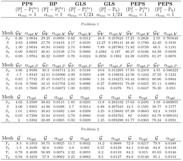
The ﬁndings of performing the DFO search on ﬁxed meshes are shown in Table

2, where we present the percentage gains and the approximations of the optimal

value for the stabilization parameters

α

_opt

, α

_opt,_V

, and

α

_opt,P

. We notice that the

optimal values achieved with the separate estimators are diﬀerent, each one providing

a signiﬁcant gain on the estimator. On the other hand, the value achieved by the

total estimator is (at least in most cases) between those two values and can provide a

signiﬁcant reduction on the estimator. The numerical results from Figures 3–5 suggest

that this reduction, of up to 80% in some cases with respect to the reference value for

α, induces a signiﬁcant gain on the error as well.

4. Selection of the stabilization parameter on a sequence of adaptively

refined meshes.

The results in the previous section are concerned with ﬁxed meshes.

We now apply the approach in the context of an adaptive mesh reﬁnement procedure,

driven using the local error indicator

(4.1)

η

_K

(α)

2

= Φ

2_c,K

+

ν

2

Φ

_nc,K2

+

Φ

∗_c,K

+

ν

Φ

_nc,K

2

,

where Φ

_c

is given by (5.21), Φ

_nc

is given by (5.22), and Φ

∗_c

is given by (5.29).

Ideally, one would optimize over

α

on every mesh constructed throughout the

adaptive reﬁnement procedure. In practice, the cost of such a procedure would be

prohibitive and, fortunately, is unnecessary. Instead we optimize the choice of

α

once

on the initial mesh, and then retain this value on all the subsequent adaptively reﬁned

meshes.

In Figures 7 and 8 we present the results obtained using both the

idealized

algo-rithm

and the proposed

practical algorithm

to approximate the same problems

consid-ered in the previous section. We deﬁne the eﬀectivity index Θ(α) =

η(α)/

|||

(

e

_V

, e

_P

)

|||

(12)

Fig. 6_._{DFO search for Problems} ₁_and ₂_{on ﬁxed meshes}S_c _andT_d_{, respectively.}

and show the performance of the algorithms for a variety of stablized methods. The

meshes used to start the algorithms are shown in Figure 9. The results show the

good behavior of the error estimator and that the performance of both algorithms

is virtually identical, indicating that the optimal choice of

α

changes little from the

value obtained based on the initial coarse mesh.

(13)

[image:13.612.74.441.132.454.2]

1597

Table 2

Percentage gainsG,G_V,GP, andαopt’s for Problem 1using the ﬁxed meshesSd,S,Sa,Sb,

andScand for Problem 2using the ﬁxed meshesTa,Tb,Tc, andTd.

PPS

BP

GLS

PEPS

(

P

2₁

−

P

cts

1

) (

P

21

−

P

cts1

) (

P

21

−

P

cts1

)

(

P

12

−

P

0

)

(

P

21

−

P

cts1

)

(

P

21

−

P

0

)

α

_rec

= 1

α

_rec

= 1

α

_rec

= 1/24

α

_rec

= 1/24

α

_rec

= 1

α

_rec

= 1

Problem 1

Mesh

G

_V

α

_opt,_V

G

_V

α

_opt,_V

G

_V

α

_opt,_V

G

_V

α

_opt,_V

G

_V

α

_opt,_V

G

_V

α

_opt,_V

Sd 6.26 3.9034 29.25 0.0956 0.82 0.0312 18.9 0.457624 17.25 0.2826 2.55 0.765648

S 2.83 2.0909 47.78 0.0418 2.17 0.0235 12.27 0.190141 48.46 0.1780 42.40 0.1816

Sa 1.36 2.0044 40.94 0.0402 2.74 0.0060 7.89 0.287962 71.82 0.0728 66.5 0.1181

Sb 0.09 0.6655 36.81 0.0138 2.74 0.0060 3.4382 0.197 86.27 0.0106 84.39 0.0039

Sc 0.69 1.9764 30.22 0.0397 0.76 0.0224 6.2856 0.1902 84.98 0.0376 81.27 0.0676

Mesh

G

_P

α

_opt,P

G

_P

α

_opt,P

G

_P

α

_opt,P

G

_P

α

_opt,P

G

_P

α

_opt,P

G

_P

α

_opt,P

Sd 3.86 2.9589 30.3 0.04714 2.33 0.0188 10.6 0.313205 17.95 0.2319 4.55 0.586223

S 1.7 1.8343 43.51 0.04906 2.99 0.0203 4.68 0.159632 42.56 0.1242 37.50 0.1422

Sa 0.85 1.7745 37.45 0.04751 2.82 0.0086 1.16 0.104272 64.44 0.0652 60.06 0.0904

Sb 0.04 0.7686 34.15 0.01704 2.82 0.0086 6.27 0.000101 79.29 0.0225 85.11 0.0001

Sc 0.45 1.7600 28.17 0.04672 1.00 0.0201 0.04 0.0476 79.1 0.0447 76.30 0.053

Mesh

G

α

_opt

G

α

_opt

G

α

_opt

G

α

_opt

G

α

_opt

G

α

_opt

Sd 4.62 3.2509 30.04 0.0515 1.85 0.0205 13.8 0.284102 17.63 0.2495 3.59 0.669955

S 2.06 1.9203 44.98 0.0498 2.7 0.0214 6.88 0.207045 44.5 0.1591 38.77 0.1577

Sa 1.01 1.8501 38.63 0.0482 1.68 0.0209 3.25 0.158682 67.39 0.0683 62.4 0.1033

Sb 0.05 0.7298 35.04 0.0163 2.78 0.0080 0.03 0.034763 82 0.0201 84.78 0.000101

Sc 2 1.8302 28.89 0.0365 0.92 0.0209 1.35 0.093298 81.77 0.0363 78.34 0.0591

Problem 2

Mesh

G

α

_opt

G

α

_opt

G

α

_opt

G

α

_opt

G

α

_opt

G

α

_opt

Ta 8.3 0.1953 50.75 0.0025 15.7 0.0032 14.2 0.0089 72.9 0.0217 79.9 0.0188

Tb 1.5 0.3189 56.6 0.005 3.9 0.005 8.57 0.0129 84.1 0.0146 84.8 0.0149

Tc 0.78 0.4039 56.89 0.0074 2.32 0.0055 8.2 0.0133 84.2 0.015 85.03 0.0146

Td 0.94 0.4219 57.9 0.0062 3.25 0.0062 9.5 0.0127 84.6 0.0146 85.1 0.0153

Idealized algorithm: Adaptive mesh reﬁnement and DFO search.

1:

Construct mesh

P

₀

. Set

i

= 0.

2:

Performing the DFO algorithm on the ﬁxed mesh

P

_i

, compute

α

(_opti)

.

3:

For each element

K

in

P

_i

, compute a local error indicator

η

_K

(α

(_opti)

).

4:

Triangle

K

is marked for reﬁnement if

η

_K

(α

(_opti)

)

≥

1₂

max

K∈Pi

η

_K

(α

(_opti)

).

5:

From step

4 deduce a new mesh using longest edge bisection reﬁnement.

6:

Set

i

←

i

+ 1 and return to step

2 .

Practical algorithm: Adaptive mesh reﬁnement and DFO search.

1:

Construct mesh

P

₀

.

2:

Performing the DFO algorithm on the ﬁxed mesh

P

₀

, compute

α

(0)_opt

and set

i

= 0.

3:

For each element

K

in

P

_i

, compute a local error indicator

η

_K

(α

(0)_opt

).

4:

Triangle

K

is marked for reﬁnement if

η

_K

(α

(0)_opt

)

≥

1₂

max

K∈Pi

η

_K

(α

(0)_opt

).

5:

From step

4 deduce a new mesh using longest edge bisection reﬁnement.

6:

Set

i

←

i

+ 1 and return to step

3 .

(14)

Fig. 7_._{Performance of the idealized and practical algorithms applied to Problem} ₁_.

5. A posteriori error estimator.

We now turn to the derivation of the error

estimator

η(α) used in the selection of the stabilization parameter.

5.1. The error equation.

Recall that

e

_V

=

u

−

u

_h

∈

H

1₀

(Ω) and

e

_P

=

p

−

p

_h

∈

L

2₀

(Ω) denote the errors in velocity and pressure, respectively, where (

u

, p) is the

solution of (2.3) and (

u

_h

, p

_h

) is the solution of (2.7). Thanks to (2.3) and (2.4), the

errors satisfy, for all

v

∈

H

1₀

(Ω) and

q

∈

L

2₀

(Ω),

(5.1)

A

(

e

_V

, e

_P

;

v

, q) =

K∈P

(

f

,

v

)

_K

−

ν(

∇

u

_h

,

∇

v

)

_K

+ (p

_h

,

∇

· v

)

_K

−

(q,

∇

· u

_h

)

_K

.

[image:14.612.93.418.93.535.2]

(15)

1599

Fig. 8_._{Performance of the idealized and practical algorithms applied to Problem} ₂_.

Fig. 9_. _{Initial meshes} S₀ _and T₀ _{for Problems} ₁ _and ₂_{, respectively, for the idealized and}

practical algorithms.

Let

{

g

_γ,K

}

be a set of equilibrated boundary ﬂuxes which are such that

g

_γ,K

∈

P

1

(γ)

2

for each

γ

∈ E

K

for all

K

∈ P

,

(5.2)

g

_γ,K

+

g

_γ,K

=

0 if

γ

=

E

K

∩ E

K

for distinct

K, K

∈ P

,

and, for all

K

∈ P

, satisfy the ﬁrst-order equilibration condition

(5.3) (

f

,

θ

)

_K

+

γ∈EK

g

_γ,K

,

θ

γ

−

ν

(

∇

u

h

,

∇

θ

)

K

+ (p

h

,

∇

· θ

)

K

= 0

∀

θ

∈

P

1

(K)

2

_.

A process to obtain such equilibrated boundary ﬂuxes will be described in section

5.3. Now, (5.2) allows us to incorporate the boundary ﬂuxes into (5.1) and integrate

[image:15.612.83.431.95.350.2]

(16)

by parts to yield

A

(

e

_V

, e

_P

;

v

, q)

=

K∈P

⎛

⎝(

r

_K

,

v

)

_K

+

γ∈EK

(

R

_γ,K

,

v

)

_γ

+ (

f

−

Π

_K

f

,

v

)

_K

−

(q,

∇

· u

_h

)

_K

⎞

⎠

(5.4)

for all

v

∈

H

1₀

(Ω) and

q

∈

L

2₀

(Ω), where the interior residuals

r

_K

∈

P

₁

(K)

2

are

given by

(5.5)

r

_K

= Π

_K

f

− ∇

p

_h

on

K,

and the boundary residuals

R

_γ,K

∈

P

₁

(γ)

2

are given by

(5.6)

R

_γ,K

=

g

_γ,K

−

ν

∇

u

_h_|_K

n

ˆ

K_γ

+

p

_h_|_K

n

ˆ

K_γ

on

γ

∈ E

_K

.

Let

≈

σ

∗

K

∈

P

2

(K)

2×2

be the unique solution to the following problem:

minimize

≈

σ

∗

K

₀_,K

subject to

≈

σ

∗

K

n

ˆ

Kγ

=

R

γ,K

on each

γ

∈ E

K

,

−

div

≈

σ

∗

K

=

r

K

in

K. Note that since integration by parts and (2.1) allow us to write (5.3) as

(5.7)

(

r

_K

,

θ

)

_K

+

γ∈EK

(

R

_γ,K

,

θ

)

_γ

= 0

∀

θ

∈

P

₁

(K)

2

,

the existence of such a

≈

σ

∗

K

follows from [29]. Moreover, integration by parts also

yields that

(5.8)

≈

σ

∗

K

,

∇

v

K

= (

r

K

,

v

)

K

+

γ∈EK

(

R

_γ,K

,

v

)

_γ

∀

v

∈

H

1₀

(Ω).

Also, let

≈

σ

_K

=

≈

σ

∗

K

−

curlζ

−

1

2 tr

≈

σ

∗

K

−

curlζ

I

,

where tr denotes the trace of a matrix,

I

is the identity matrix, and

ζ

∈

H

1₀

(K)

∩

P

3

(K)

2

is such that

≈

σ

K

₀,K

is minimized. From [27], we know that

(5.9)

≈

σ

_K

,

∇

v

K

= (

r

K

,

v

)

K

+

γ∈EK

(

R

_γ,K

,

v

)

_γ

∀

v

∈

X

.

Formulas for the quantities involving

≈

σ

∗

K

and

σ

≈K

which are required to compute our

estimator, namely,

≈

σ

∗

K

₀_,K

and

≈

σ

K

0,K

, are given in section 5.4.

5.2. Guaranteed upper bounds for the errors.

In order to obtain a

guar-anteed upper bound for the errors we use the Helmholtz-type decomposition of the