City, University of London Institutional Repository
Citation: Carrillo-Ureta, G.E. (2003). Optimal control of fermentation processes. (Unpublished Doctoral thesis, City University London)
This is the accepted version of the paper.
This version of the publication may differ from the final published version.
Permanent repository link: http://openaccess.city.ac.uk/7584/
Link to published version:
Copyright and reuse: City Research Online aims to make research outputs of City, University of London available to a wider audience. Copyright and Moral Rights remain with the author(s) and/or copyright holders. URLs from City Research Online may be freely distributed and linked to.
OPTIMAL CONTROL OF FERMENTATION
PROCESSES
By
Gabriel Eduardo Carrillo-Ureta
A Thesis submitted for the Degree of
Doctor of Philosophy
City University, London
Control Engineering Research Centre
School of Engineering
Northampton Square
London ECI V OHB
United Kingdom of Great Britain
TABLE OF CONTENTS
Page
List of Tables... )
List of Figures... 6
Acknowledgements. . . 11
Declaration... 12
Abstract. ... ... ... ... ... . .. ... . .. ... ... ... ... .. ... ... ... ... ... ... ... 13
List of Abbreviations. . . 14
Chapter I: Introductory Terms and Basic Concepts... 15
1.1 Aims and Objectives of the Thesis... ... .... 15
1.2 Introduction to Beer Fermentation... ... ... ... ... .. . .. ... .. . ... .... 17
1.3 Optimal Control and Optimisation Algorithms... ... 23
1.4 Summary... ... ... ... ... .. . .. .. . ... ... ... 29
Chapter II: Modelling and Simulation of Beer Fermentation Processes... 30
2.1 Modelling of Fermentation Processes... ... 30
2.3 Computer Simulation of the Selected Fermentation Process... ... .f9
2.4 Summary... ... ... 56
Chapter III: Approach to Optimal Control... 57
3.1 Introduction to the DIS OPE Algorithm... ... 57
3.2 Optimisation of the Beer Fermentation Process... ... 63
3.2.1. Optimal Steady-State Solution... 67
3.2.2. Application of Calculus of Variations ... 71
3.3 Gradient Method in Function Space... ... 75
3.4 The DISOPE Algorithm... ... ... ... ... ... 84
3.5 Summary... .... 98
Chapter IV: Genetic Algorithms ... . 99
.f. 1 Introduction to Genetic Algorithms ... '" ... .. 99
4.-' 0 ' " ptImIsatlOn uSIng enetIc . G 'AI'hm gont s ... '" ... . 104
.f.3 Genetic Algorithms applied to the Beer Fermentation Process ... . 107
.f . .f Summary ... . 12.f Chapter V: Sequential Quadratic Programming (SQP)... 125
5.1 Non-Linear Progran1n1ing \vith Constraints... 125
....
5.2 Sequential Quadratic Programming... ... 129
5.3 SQP Implementation in MATLAB... ... 137
5.3.1. Updating The Hessian Matrix of the Lagrangian function... ... 137
5.3.2. Quadratic Programming Problem Solution... 138
5.3.3. Line Search and Merit Function Calculation... 1.+2 5.4 SQP for Optimal Control of Beer Fermentation... ... ... 1.+3 5.5 Summary... ... 155
Chapter VI: Final Remarks... 156
6.1 Comparison of the Methods Reviewed... .... ... ... 158
6.2 Conclusions and Further Work... ... 163
6.3 List of Conferences and Publications from this Research... . . . 165
Appendix A The Genetic Algorithms Toolbox Functions Described... ... . .. ... . . 166
Appendix B System Identification using MA TLAB. . . ... . . .. 180
Appendix C System Identification with Neural Networks... 188
LIST OF TABLES
Page
Table 2.1 Nomenclature used for the different relationships... ... 31
Table 2.2 Description of the parameters used in fed-batch fermentation... 37
Table 2.3 Growth models found in biotransformations... 39
Table 2.4 Nomenclature in the mathematical modeL... 44
Table 2.5 Results after the simulation of the beer modeL... 55
Table 3.1 Nomenclature used... ... 63
Table 3.2 Results corresponding to optimum steady-state control profile... ... 71
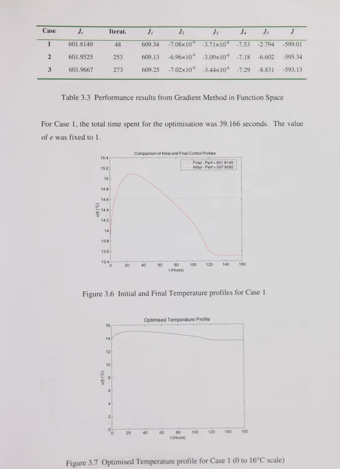
Table 3.3 Performance results from Gradient Method in Function Space... ... 77
Table 3.4 Performance results from the DIS OPE Algorithm... ... 90
Table 4.1 Technical terms used in GA literatures... ... 102
Table 4.2 Results obtained with GA for Cases 1 to 12... ... 110
Table 4.3 New results obtained with GA for Cases A to L... ... ... ... 117
Table 5.1 The necessary and sufficient conditions for x* to be a local minimum of the general constrained non-linear programming problem. 130 Table 5.2 Default parameters used by the Optimisation Toolbox... ... 146
Table 5.3 Changed parameters used for the SQP optimisation... ... 146
Table 5.4 Results of the optimisation with SQP for Cases 1-10... ... 148
Table 5.5 Results from the optimisation of the Case #6... .... 148
Table 5.6 Results of the optimisation with SQP for Cases A-G... ... 152
Table 5.7 Results from the optimisation of the Case F... ... ... 152
Table 6.1 Summarised results with the optimisation algorithms considered... 158
LIST OF FIGURES
Page
Figure 2.1 Experimental set-up... .+2
Figure 2.2 Process scheme for the kinetic modeL... 43
Figure 2.3 SIMULINK Model of the Beer Fermentation Process... .+9
Figure 2.4 Temperature Profile used in the Beer Industry... 50
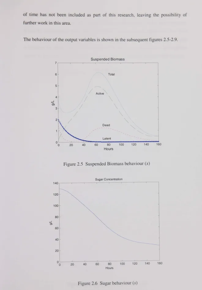
Figure 2.5 Suspended Biomass behaviour (x)... ... 51
Figure 2.6 Sugar behaviour (s)... 51
Figure 2.7 Ethanol behaviour (e)... ... 52
Figure 2.8 Ethyl Acetate behaviour (acet)... 52
Figure 2.9 Diacetyl behaviour (diac)... ... 53
Figure 2.10 Objective Function value to be maximised... .. ... ... .. ... 5.+
Figure 3.1 State response x I for the optimum steady-state profile... ... ... . .. ... 68
Figure 3.2 State response X2 for the optimum steady-state profile... 69
Figure 3.3 State response X3 for the optimum steady-state profile... 69
Figure 3.4 State response X4 for the optimum steady-state profile... 70
Figure 3.5 SIMULINK Model for the steady-state case... 70
Figure 3.6 Initial and Final Temperature profiles for Case 1... 77
Figure 3.7 Optimised Temperature profile for Case 1 (0 to 16°C scale)... 77
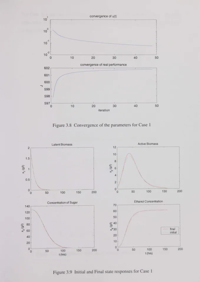
Figure 3.8 Convergence of the parameters for Case 1... 78
Figure 3.9 Initial and Final state responses for Case 1... 78
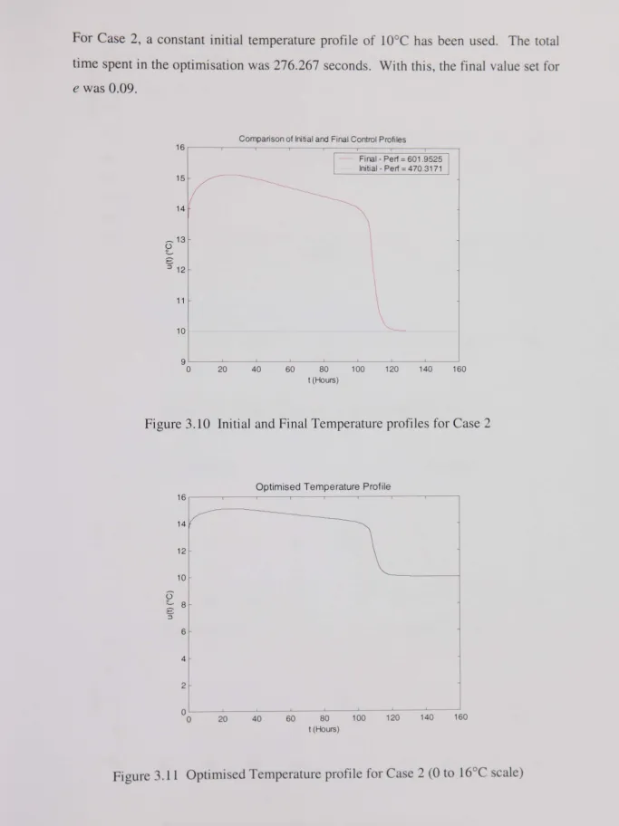
Figure 3.10 Initial and Final Temperature profiles for Case 2... 79
Figure 3.11 Optimised Temperature profile for Case 2 (0 to 16°C scale) ... 79
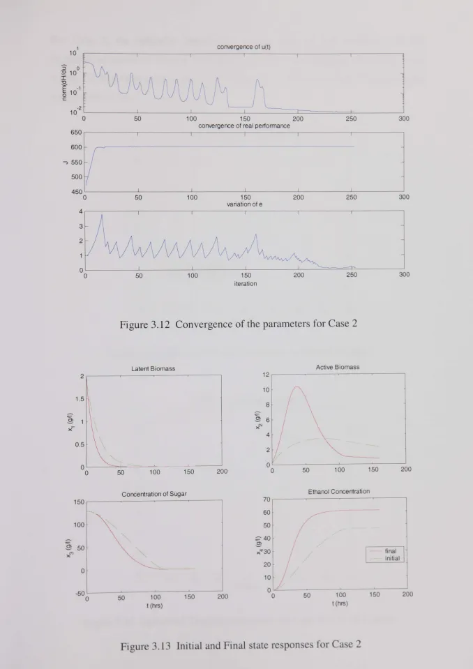
Figure 3.12 Convergence of the parameters for Case 2.. .. .. .. .. .. ... .. .. ... .. ... 80
Figure 3.13 Initial and Final state responses for Case 2.. .. .. .. . .. .. .. .. .. .. .. .. .... 80
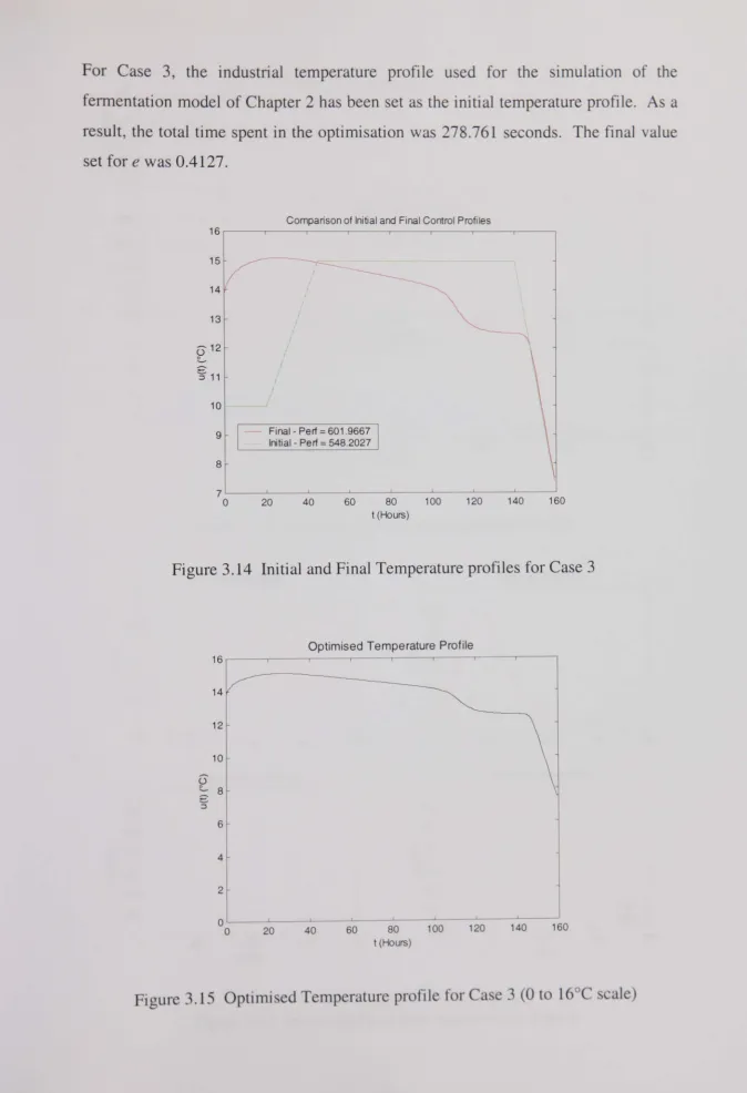
Figure 3.14 Initial and Final Temperature profiles for Case 3... ... ... 81
Figure 3.15 Optimised Temperature profile for Case 3 (0 to 16°C scale) ... 81
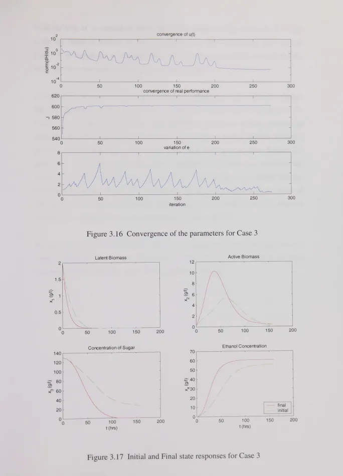
Figure 3.16 Convergence of the parameters for Case 3.. ... ... .... .. .. .. .. .. .. .. .... 82
Figure 3.17 Initial and Final state responses for Case 3.. ... .... ... ... 82
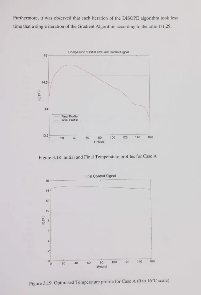
Figure 3.18 Initial and Final Temperature profiles for Case A... 91
Figure 3.19 Optinlised Temperature profile for Case A (0 to 16°C scale)... 91
Figure 3.20 Convergence of the parameters for Case A... 92
Figure 3.21 Initial and Final state responses for Case A... ... 9'
Figure 3.22 Initial and Final Temperature profiles for Case B... 93
Figure 3.23 Optimised Temperature profile for Case B (0 to 16°C scale).. ... 93
Figure 3.24 Convergence of the parameters for Case B ... 94
Figure 3.25 Initial and Final state responses for Case B. . . .. . . . 94
Figure 3.26 Initial and Final Temperature profiles for Case C... 95
Figure 3.27 Optimised Temperature profile for Case C (0 to 16°C scale)... 95
Figure 3.28 Convergence of the parameters for Case C... .. .... .... .. .. .. .. ... 96
Figure 3.29 Initial and Final state responses for Case C... 96
Figure 4.1 A possible classification of Search Techniques... 103
Figure 4.2 SIMULINK model "beemew" for the fermentation process... 108
Figure 4.3 Profile for Case #1... 110
Figure 4.4 Profile for Case #2... 110
Figure 4.5 Profile for Case #3... ... ... ... ... .... .. .. ... ... III Figure 4.6 Profile for Case #4... III Figure 4.7 Profile for Case #5. .. . . . .. . . .. . . .. . . III Figure 4.8 Profile for Case #6... 111
Figure 4.9 Profile for Case #7... 111
Figure 4.10 Profile for Case #8... ... ... ... .. ... .. ... III Figure 4.11 Profile for Case #9... ... ... ... ... ... .. . ... ... ... ... .. . III Figure 4.l2 Profile for Case #10... III Figure 4.13 Profile for Case #11... 112
Figure 4.14 Profile for Case #12... ... ... ... ... 112
Figure 4.15 Jvalues for Case #1... ... ... ... ... 112
Figure 4.16 Jvalues for Case #2... 112
Figure 4.17 J values for Case #3... ... ... 112
Figure 4.18 Jvalues for Case #4... 112
Figure 4.19 J values for Case #5... 113
Figure 4.20 J values for Case #6... 113
Figure 4.21 J values for Case #7... 113
Figure 4.22 Jvalues for Case #8... 113
Figure 4.23 J values for Case #9... ... ... ... ... .. .. .. ... 113
Figure 4.24 Jvalues for Case #10... 113
Figure 4.25 J \'alues for Case # 11... 113
Figure 4.26 J \'alues for Case #12... 113
Figure 4.27 Smoothed Temperature (OC) vs. Time (Hours)... 115
Figure 4.28 Suspended Biomass Behaviour for Case #7... . .. .... .... . .. . . .. ... ... 115
Figure 4.29 Concentration of Sugar and Ethanol for Case #7... ... ... ... 116
Figure 4.30 Ethyl Acetate Concentration for Case #7... ... 116
Figure 4.31 Diacetyl Concentration for Case #7... ... ... 116
Figure 4.32 J values for Case A.. ... ... .... .. ... .. .... .. .... ... 118
Figure 4.33 Profile for Case A... ... ... ... 118
Figure 4.34 J values for Case B... .. ... ... ... ... ... 118
Figure 4.35 Profile for Case B... 118
Figure 4.36 J values for Case C... 118
Figure 4.37 Profile for Case C.. .. .. .. .. .. .. .. .. .. .. .. .. .. .. .. .. .. .. .. .. .. .. .. .. .... .. .. 118
Figure 4.38 Jvalues for Case D... 118
Figure 4.39 Profile for Case D... ... 118
Figure 4.40 Jvalues for Case E... 119
Figure 4.41 Profile for Case E... 119
Figure 4.42 J values for Case F... ... ... .. .. .. ... ... .. .... ... 119
Figure 4.43 Profile for Case F... ... ... .... .. ... ... 119
Figure 4.44 J values for Case G.. .... .. .... .. .... .. .. .. .. .. .. .. .... .. .. .. .. .. .. .. .. ... 119
Figure 4.45 Profile for Case G... 119
Figure 4.46 J values for Case H... ... .... .. .. ... .. ... ... 119
Figure 4.47 Profile for Case H... .... .. .... .. ... ... ... ... .. .... ... . .. .. ... .. .. 119
Figure 4.48 Jvalues for Case I... 120
Figure 4.49 Profile for Case I... ... ... ... .. .... ... ... ... ... .... .... 120
Figure 4.50 Jvalues for Case
J... ... ... ...
120Figure 4.51 Profile for Case J... 120
Figure 4.52 J values for Case K... ... ... .... .. .... .. ... ... 120
Figure .+.53 Profile for Case K... ... ... ... ... .. .... 120
Figure -1-.54 Jvalues for Case L ... 120
Figure .+.55 Profile for Case L... 120
Figure .+.56 Suspended Biomass Behaviour for Case J... 121
Figure -1-.57 Ethanol Concentration for Case J... 121
Figure -1-.58 Sugar Concentration for Case J... 122
Figure .+.59 I·:thyl Acetate Concentration for Case J... 122
Figure .+.60 Diacctyl Concentration for Case J... ... 122
Figure 5.1 SIMULINK model used for the SQP optimisation... ... ... ... 1-+5
Figure 5.2 Initial and Optimised Temperature Profiles for Case #6... 1-+8
Figure 5.3 Development of the SQP algorithm for Case #6... 1-+9
Figure 5.4 Suspended Biomass behaviour for Case #6... 150
Figure 5.5 Sugar and Ethanol Concentration for Case #6... 150
Figure 5.6 Ethyl Acetate Concentration for Case #6... 150
Figure 5.7 Diacetyl Concentration for Case #6. . . .. . . .. . . . .... 151
Figure 5.8 Initial and Optimised Temperature Profiles for Case F.. ... 153
Figure 5.9 Development of the SQP algorithm for Case F... ... ... 153
Figure 6.1 Industrial Temperature profile used in practice... 159
Figure 6.2 Temperature profile obtained with the Golden Section Search Method... 159
Figure 6.3 Temperature profile obtained with the Gradient Method in Function Space... 160
Figure 6.4 Temperature profile obtained with the DIS OPE Algorithm... 160
Figure 6.5 Temperature profile obtained with Genetic Algorithms.... .. ... 160
Figure 6.6 Temperature profile obtained with Sequential Quadratic Programming. . . ... 161
Figure B.l SIMULINK Model used for System Identification... ... ... ... ... 180
Figure B.2 Data Plot of Latent Biomass.. . ... ... . . ... ... ... ... ... ... .. .. 184
Figure B.3 Data Plot of Active Biomass... 184
Figure B.4 Data Plot of Dead Biomass... 184
Figure B.5 Data Plot of Sugar Concentration... 184
Figure B.6 Data Plot of Ethanol Concentration... ... ... ... ... ... 185
Figure B.7 Data Plot of Ethyl Acetate Concentration. .. . . .. . . ... 185
Figure B.8 Data Plot of Diacetyl Concentration... 185
Figure B.9 Data Plot for the Objective Function... 185
Figure B.l 0 Response of Latent Biomass... 186
Figure B.l1 Response of Active Biomass... ... ... ... .. . ... ... .. . . . ... 186
l:igure B.1 ~ Response of Dead Biomass ... '" ... .... .. ... 186
Figure B.13 Response of Sugar... 186
Figure B.l-+ Response of Ethanol. .. ... .. .... ... ... ... ... . ... 186
Figure B.15 Response of Diacdyl... ... .... .. ... .. .... .. ... .... .... ... 186
Figure B.16 Response of Objccti\\.~ Function... 186
Figure B.17 Response of Temperature Profile... .... 186
Figure C.1 The basic system identification procedure... 188
Figure C.2 SIMULINK model with input data "ut", resulting in output data "yt"... . . . 189
Figure C.3 SIMULINK model with input data "uv", resulting in output data "yv"... . . .. 189
Figure CA Graphs representing Input/Output Sequence 1 (ut and yt)... 190
Figure C.5 Graphs representing Input/Output Sequence 2 (uv and yv)... 190
Figure C.6 The order index criterion evaluated for different lag spaces... 191
Figure C.7 The order index vs lag space and the recommended choice... 192
Figure C.8 The NNARX model structure used for the beer model... 192
Figure C.9 Output Sequence 1 (yt) and the one step ahead prediction... 193
Figure C.1 0 Output Sequence 2 (yv) and the one step ahead prediction... 194
Figure C.11 Auto and Cross Correlation graphs for Input/Output Sequence l.... 195
Figure C.12 Auto and Cross Correlation graphs for Input/Output Sequence 2.... 195
Figure C .13 Input Sequence 1 and Error Values after pruning. . . 196
Figure C.14 Input Sequence 2 and Pruned Neural Network connections... 197
Figure C.l5 Output Sequence 1 and the one step ahead prediction... 198
Figure C.16 Output Sequence 2 and the one step ahead prediction after prunIng. . . 1 98 Figure C.17 Auto and Cross Correlation graphs for Input/Output Sequence 1 after pruning. . . 199
Figure C.18 Auto and Cross Correlation graphs for Input/Output Sequence 2
after pruning. . . 1 99
ACKNOWLEDGEMENTS
I wish to express my sincere thanks to my supervisor Professor Peter D. Roberts for
his help throughout these four years. A special thanks to Dr. Victor Becerra for his
unconditional assistance. Without them this could not be possible.
Also thanks to all my good friends in the Electrical Engineering Department: Daniel.
Lackson (R.LP.), Ziad, Stavros, Ermioni and Moufid because they have been great
friends during my PhD life. Not forgetting Joan and Linda for their good advises and
support.
My sincere gratitude to all my family in Panama, in particular: my father Daniel, my
mother Vielka and my sister Michelle for always supporting me in everything that I
do; and happiness for the newest member of our "next generation", my niece
Melanie. A very special mention to my girlfriend Amy for her support during the
final study years, her encouragement and patience will always be deeply appreciated.
Also thanks to lng. Roberto Barraza and Dr. Emir Humo in the Universidad
Tecnologica de Panama for their valuable advise.
But above all, thanks to God for leading my steps every day of my life and giving me
the opportunity to be where I am now; without Him these studies could not be
possible at all: thanks for everything.
DECLARATION
The author grants power of discretion to the University Librarian to allow the thesis
to be copied in whole or in part without further reference to the author. This
permission covers only single copies made for study purposes, subject to normal
conditions of acknowledgement.
ABSTRACT
The general purpose of this thesis is to focus on a particular industrial process (from the beer industry) which serves as a guidance example for optimal control using different algorithms/methods. At the same time, the aim is to demonstrate the capabilities/features of MATLAB and SIMULINK as tools used in programming algorithms and simulation for optimal control of non linear systems. The thesis shows how to approach an optimisation problem with different techniques and to compare them on the same basis.
The main reasons for carrying out research on a beer fermentation process can be summarised as follows: this kind of industry represents an up-to-date example of industrial processes in general, the need to compare and evaluate optimisation methods (well established and "modern") on similar circumstances using the sanle process model and finally, give a good foundation for the control engineer to follow-up this work with different optimisation techniques and/or any other industrial process.
The fundamental features of the methods used involve the viability of known previously tested algorithms for optimal control of beer processes with high non-linearity and constraints; thus testing the flexibility of some of the known MA TLAB Toolboxes for the optimal control of a particular simulated mathematical model.
An important aspect of the experimentation that has been carried out, is the creation of a simulated model of a selected beer process by means of including the mathematical equations, parameters and initial conditions into an s-function block. This SIMULINK model also incorporates the particular objective function that can be calculated directly after the simulation of the process for a particular input temperature profile. Together with the use of some available MA TLAB functions for the formulation of particular optimal control techniques, this facilitates the creation of program routines that can be interfaced with the simulated process.
The final results using different optimisation methods such as: the gradient method in function space, DIS OPE algorithm, Genetic Algorithms and Sequential Quadratic programming; show substantial improvement in the perfomance index obtained. The optimised temperature profiles found can be implemented for industrial application to provide a maximised ethanol production under particular restrictions, i.e. final
by-products concentration, contamination risk and brisk changes in temperature.
Abbreviation ARX CPU DISOPE DMS EOP EQP FPE GA HGA IQP KKT LP MB MHz MO MOP MMOP NLP NN OBS PC PEM QP RAM ROP SO SQP TSP VOl'.
LIST OF
ABBREVIATIO~VSExplanation
Auto regressive eXternal input
Central Procesing Unit
Dynamic Integrated System Optimisation and
Parameter Estimation
Dimethyl Sulphide
Expanded Optimal control Problem
Equality constrained Quadratic Programming
Final Prediction Error
Genetic Algorithms
Hybrid Genetic Algorithm
Inequality constrained Quadratic Programming
Karush-Kuhn-Tucker
Linear Programming
Mega Bytes
Mega Hertz
Multi-Objective
Model based Optimal control Problem
Modified Model based Optimal control Problem
Nonlinear Optimisation Problem
Neural Networks
Optimal Brain Surgeon
Personal Computer
Prediction Error Method
Quadratic Programming
Random Access Memory
Real Optimal control Problem
Single-Objectiye
Sequential Quadratic Programming
Tran?lling Salesman Problem
Vicinal Oiketone
CHAPTER I
INTRODUCTORY TERMS AND BASIC CONCEPTS
Beer fermentation including some basic concepts is going to be the main focus of
this chapter. Definitions of some introductory terms will help to understand the
parameters related to this work. Optimal control techniques are also a main point of
discussion and will be introduced for an initial understanding on how optimisation
techniques work.
1.1 AIMS AND OBJECTIVES OF THE THESIS
The main aims and objectives of the research can be summarised as follows:
• To improve the results obtained previously by Andres-Toro et al (1997a)
concerning the optimisation of the beer process model, herewith obtain an even
superior objective function value. Together with this, show how other
optimisation techniques can provide a better understanding of the process
behaviour.
• To present a useful introduction on the importance of selecting an appropriate
mathematical model as the starting point for optimal control, this without
considering a too complicated (that cannot be properly optimised) or a too simple
one (that does not follow the real behaviour closely).
• To design general MA TLAB scripts for different optimisation techniques that are
simple, flexible and adaptable for the optimal control of any industrial process
simulated from a mathematical model.
• To obtain an implementable optimised temperature profile that can be used in the
beer making industry. This can be achieved by applying a smoothing technique
when needed to make the profile functional.
• To n1ake a comparison of some known (also considering new and/or modified
approaches) optin1isation methods and techniques under similar conditions and
give some advice on how to choose the most suitable algorithm for a particular
process.
A list of the literature reviewed from previous work related to this thesis has been
included as an initial reference to some background infonnation:
• The main beer fennentation model considered for optimal control has been
created from previous work by Andres-Toro et al (1998).
• The book "Optimal Control in Fennentation Processes" by Leigh (1986) has
been used for consultation and review at the beginning of this research.
• Other mathematical models of fennentation processes have been considered
useful in the first stages of the research as an insight on different approaches
to model real industrial processes. A review on these papers has been
included in the MPhil to PhD transfer report (Carrillo-Ureta, 1999).
• For every particular optimisation technique/method, papers on the different
algorithms used and its application to particular cases have been reviewed:
the principles behind the Gradient Method in Function Space have been
considered from the book by Noton (1972); for the case of the DISOPE
algorithm, work by Roberts (1993) and Becerra and Roberts (1995); the use
of the Genetic Algorithms Toolbox by Chipperfield et al (1999) has been
reviewed from work by Chishimba (1998); and finally, the Sequential
Quadratic Programming algorithm under MA TLAB has been examined from
the Optimization Toolbox Manual (Coleman et aI, 1999).
1.2 INTRODUCTION TO BEER FERMENTATION
In order to produce beer, water and barley are mixed together to generate a s\\eet
infusion, the wort; this is then blended with hops and later fermented with yeast.
This may look as a simple procedure but in practice it can be extremely complicated.
Yeast is a single celled microorganism that transforms the sugar in the wort into
alcohol and carbon dioxide (it reproduces by maturing). There are actually hundreds
of varieties and strains of yeast and in general each brewery has its own variety.
which principally determines the particular beer character.
The term "fermentation" is derived from the Latin verb fervere, that means to boil,
thus describing the appearance of the action of yeast on extracts of fruit or malted
grain (Stanbury et aI, 1995). For some yeast varieties, the cells go up to the top at the
end of the fermentation, giving the name of top fermentation (ales are brewed like
this). On the other hand, when at the end of fermentation the yeast cells fall to the
bottom, bottom fermentation is achieved (used for lager or pils). Earlier, there were
just two types of beer yeast: ale yeast (the top-fermenting type: Saccharomyces
cerevisiae) and lager yeast (the bottom-fermenting type: Saccharomyces uvarum.
previously known as Saccharomyces carlsbergensis). Nowadays, as a result of
recent reclassification of Saccharomyces species, both ale and lager yeast strains are
considered to be members of Saccharomyces cerevisiae.
Fermentation has come to have different meanings to biochemists and to industrial
microbiologists. Its biochemical meaning relates to the generation of energy by the
catabolism of organic compounds, whereas, its meaning in industrial microbiology
tends to be much broader. Brewing and the production of organic solvents may be
described as fermentation in both senses of the word but the description of an aerobic
process as fermentation is obviously using the term in the microbiological context.
Even though beers are brewed from related resources. beers throughout the \vorld
have their own individual styles. Their distinctiveness comes from the mineral
content of the water used. the types of ingredients employed, and the difference in
bre\\ing lnethods. Nonetheless. it can be said that there are two established beer
stvles: ales and lagers. Ho\n:ver. in addition to ales and lagers, there are other
classical beer styles such as wheat beers, porters, stouts, and Iambics that are worth
mentioning. Albeit most of the classical beer styles originated in Europe (Belgium.
British, Czech Republic, French, German and Irish just to mention the most
important), many of them are brewed effectively all over the world. With any beer
technique there are no unbreakable policies and variations within flavour.
ingredients, and methods of brewing for different styles are to be expected.
Brewmasters each have their own explanation of what they consider suitable for the
style.
According to Goldammer (2000), malt influences the flavour of beer more than any
other ingredient: the malt types selected for brewing will determine the final colour,
flavour, mouth feel, body, and aroma. As regards on the style of beer desired and the
type of malt, it takes from 15 to 17 kg of malt to produce a hectolitre of beer. There
is no general structure used for classifying malts since "maltsters" classify and
advertise their products in their own way. Though regularly malts are classified as:
base malts (Pilsner malt, Pale Ale malt and Mild Ale malt), specialty malts
(light-coloured: Vienna malt and Munich malt; dark-(light-coloured: Amber malt and Brown
malt), caramelised/crystal malts (Dextrin malts), roasted malts (Chocolate malt and
Black malt), unmalted barley (Roasted barley), and other malted grains (Wheat malt
and Rye malt).
Wheat malt, understandably, is essential in making wheat beers. Wheat is also used
in malt-based beers for the reason that its protein gives the beer a pleasant mouth
sensation and improves beer head stability. As a negative aspect, wheat malt
contains significantly more protein than barley malt, around 13 to 180/0 more, and
consists primarily of glutens that can result in cloudy beer. European wheat malts
have generally a smaller amount of enzymes than American malts, perhaps because
of the malting methods or the varieties of wheat used.
The conventional way for beer fermentation is to add yeast to the worth and wait for
.
.some time. letting the yeast consume substrates and produce ethanol (without
stirri ng). According to the industry, lager yeast strains are best used at temperatures
ranging from 7 to 15°C. Here\vith. lager yeasts develop slower than ale yeasts. and
\vith less surt:lCe fOaIH they tend to settle down to the bottom of the fermentor clu~e
to the end of the fermentation (referred to as bottom yeasts). The ultimate flavour of
the beer depends significantly on the strain of lager yeast and the temperatures at
which it was fermented. Thus, fermentation can be accelerated with an increase of
temperature but, however, some contamination risks (Lactobacillus, etc.) and
undesirable by-products (diacetyl, ethyl acetate, etc.) could appear.
Defining the flavour and aroma of beer can be very difficult, this arises as a result
from a large selection of parameters that come up from a number of different
sources. Malt, as mentioned before, hops, and water have a great impact on the beer
flavour, the decomposition of yeast which forms by-products during fermentation
and maturation, is in addition essential (Goldammer. 2000). The most distinguished
of these by-products are certainly ethanol and carbon dioxide; however additionally.
a great amount of other flavour compounds are also formed:
a) Esters are among the most significant aroma components in beer, regarded of
imparting a fruity quality to beer. As indicated by the production companies,
esters are more desirable in ales than in lagers. Ester production can be
increased by several factors including: high fermentation temperatures;
restricting wort aeration; increasing the attenuation limit; and also increasing
the wort concentration. Additionally, the type of yeast has an effect on ester
concentration.
b) Diacetyl can be classified as a ketone and has also an important significance
to beer flavour and aroma. Together with another ketone 2,3-pentanedione.
these are described as the vicinal diketone (VDK) content of beer, which is
the primary flavour in differentiating aged beer from green beer. Even so,
diacetyl is critical because it is produced in larger quantities and also having a
larger influence in the beer flavour than 2,3-pentanedione. The existence of
diacetyl manifests with a buttery flavour typically, whereas 2,3-pentanedione
has more of a honey taste. The flavour of diacetyl can firstly be confused
with the taste of caramel malts. but afterwards it can be distinguished:
diacetyl frequently tends to be unbalanced in most beers. re\"caling a rough
fla\"our; the fla\"ouring inlparted hy caramel malts con\"crscly. is likely to hL'
stable.
c) More than a few active aldehydes can affect the beer flavour. Aldehydes in
beer can be produced during brewing at different periods by means of the
oxidation of alcohols and various fatty substances. They are reduced to
ethanol by the end of the primary fermentation. If oxygen is introduced back
into the process, then the ethanol is oxidized back into acetaldehyde. Kunze
(1996) affirms that the production of acetaldehyde can be increased by
different factors: a fast fermentation; rise of the temperature throughout the
fermentation; low wort ventilation; and infected worts (particularly by
varieties of Zymomonas anaerobia). Just like with diacetyl, the incidence of
active yeast in the maturation stage is a requirement for adequately little
aldehyde levels in the final product. By means of a warmer maturation phase,
aldehydes can be avoided with ease.
d) Organic and inorganic sulphur volatiles for instance hydrogen sulphide,
dimethyl sulphide, sulphur dioxide, and thiols can have an effect on the beer
flavour. Sulphur compounds can be tolerable or still desired if present in
lesser amounts, but can increase to distasteful off-flavours (rotten egg
flavour) in larger concentrations. Three important basic ingredients of
sulphur in beer are: untreated resources (malt and/or hops), yeast metabolism,
and spoilage organism.
e) Another wanted flavour compound in lager beer (not desirable in ales) and
accountable for malty/sulphuric taste is the dimethyl sulphide (DMS). DMS
can, in addition, improve the malt integrity of the beer. It is known in the
industry that malting process itself have more repercussion on beer DMS
quantities than the conditions surrounding the fermentation. It is also
acknowledged that reduce fermentation temperatures and increasing wort
gravity help DMS production.
f) Fusel alcohols are another kind of by-products that playa part directly to beer
flavour (sometimes referred to as higher alcohols). Also important because
of their involvement in ester formation. They enclose strong flavours.
producing an "alcoholic" or "solvent-like" scent (known to kave a \varming
effect on the palate). According to its production, the yeast strain seems to be
very significant, some being able to produce up to three times as much fusel
alcohols as others. Another factors that increase the production of fusel
alcohols are: high fermentation temperatures, mutant yeasts, high wort
gravities, intensive aeration of the pitching wort, and low amino acid
concentration in wort.
g) Organic acids can be derived from malt and are present at low leyels in \\·ort.
nonetheless, their concentration increases during the beer fermentation.
Some other acids are produced exclusively as a consequence of yeast
metabolism. They can directly affect the flavour of beer by decreasing its pH
level.
h) Fatty acids are low-grade components of wort but can increase in
concentration during fermentation and maturation. They lead to goaty,
foamy, or fatty flavours and are renowned as ordinary flavour features in both
lagers and ales; however, they are well established in lagers because of the
predisposition of some lager yeast strains to generate greater quantities of
fatty acids than do strains of ale yeast.
i) Yeast also produces some nitrogen compounds during fermentation and
maturation such as amino acids and lower peptides, with this contributing to
shape the flavour and provides an increase in palate roundness. F or that
reason, collecting the yeast too soon can yield empty, dry beers even if
lagered afterwards for a extended period.
The right selection of yeast with the basic brewing characteristics needed is essential
from a product quality and economic point of view. The criteria for yeast selection
can be different in accordance to the requirements of the brewing facilities and the
beer style, but they are expected to incorporate the follo\\"ing aspects:
• fast fermentation~ • Ycast stress tolerance:
• tlocculation;
• rate of decrease at the temperature wanted;
• flavour of the final product;
• superior yeast storage features;
• stability against mutation; and
• stability against degeneration.
Fermentation time/temperature profiles vary extensively throughout the industry for
beer lagers. Conventional lager brewing comprises pitching the yeast between 5 and
6°C letting the temperature to increase between 8 and 9°C. This usually results in a
beer with improved quality since low fermentation temperature slows down the
development of by-products, esters, fusel alcohols, and diacetyl, all of which can be
inappropriate in lagers (as mentioned before). On the other hand, the lag period is
normally longer at lower fermentation temperatures. At the end of primary
fermentation the temperature can be reduced by one to one and a half degrees Celsius
per day and relocated to a lager cellar where kept between 4 and 5°C. Although
frequently the yeast is pitched between 7 and 8°C and after a few days the
temperature is increased to 10 or 11°C. Other breweries tend to use the same initial
temperature but then increased to 14 and 15°C. A number of brewers are
acknowledged to pitch between 12 and 14°C and then raise the temperature to 18°C.
Microorganisms causing spoilage during brewing and beer processing are limited to
a few varieties of bacteria, wild yeasts, and molds. This is thanks to the beer being a
somewhat hostile growth medium for most beer spoilage microorganisms. The
alcohol content, low pH, and the presence of hop constituents are inhibitory, while
the lack of nutrients limits the development of those cells that do survive.
Nevertheless, these can interfere with the fermentation itself or have damaging
effects on beer flavour and shelf life.
1.3 OPTIMAL CONTROL AND OPTIMISATION ALGORITH\lS
The ancient Egyptians were the first to brew beer. The earliest true large-scale
breweries date from the early 1700s when wooden vats of 1500 barrels capacity \yere
introduced. Even some process control was attempted in these early breweries. as
indicated by the recorded use of thermometers in 1757 and the development of
primitive heat exchangers in 1801. During the late 1800s Hansen started his
pioneering work at the Carlsberg brewery and developed methods for isolating and
propagating single yeast cells to produce pure cultures and established sophisticated
techniques for the production of starter cultures (Seborg et aI, 1989).
Biotechnological processes, as the fermentation one, may be conveniently classified
according to the mode chosen for process operation: either batch, fed-batch or
continuous (Johnson, 1987). During batch operation of a process, no substrate is
added to the initial charge nor is product removed until the end of the process.
Nevertheless, continuous operation is more economic, where substrate is continually
added and product continually removed. Fed-batch processes introduce the greatest
challenge since the feed rate may be changed during the process but no product is
removed until the end.
The heuristic method of trial and errOL which is used to find an optimal or
pseudo-optimal operating regime by manipulating the process technological parameters, is
one of the oldest optimisation methods. According to Stengel (1994), there are in
general three reasons for process control: to ensure or enhance process stability, to
suppress the influence of disturbances and finally to optimise the process
performance. The formulation of an optimal control problem requires the following
components (Stanbury et aL 1995):
i) A l110del of the system to be controlled: this is the constitutiye equations.
together where applicable with end-state conditions and response transformation.
It characterises the system and enables the effect of all iteratiYe controls on the
ii) The constraints upon the design: they limit the range of permissible solutions
and fix many systems properties.
iii) The demands presented to the system as a design goal (objective. criterion or
index): is derived from a design value statement. The problem is to decide the
control that gives the least or greatest value of this index.
Many control design problems are based on two phases: choosing a control structure
and choosing an optimal set of parameters given the control structure, although a
design process may pass repeatedly through these two phases (Queeinec et al, 1992).
The parameters are chosen to satisfy a set of inequalities specifying design objectives
or to minimise a criterion subject to those inequalities.
The control of a fermentation process is based on the measurement of physical,
chemical or biochemical properties of the fermentation broth and the manipulation of
physical and chemical environmental parameters such as temperature, dissolved
oxygen tension and nutrient concentrations (Omstead, 1990). The microorganisms
or biomass concentrations are the central feature of fermentation affecting the rates
of growth, substrate consumption and product formation.
Czyzyk et al (1997) state that numerical optimisation methods can be divided in two
major sub fields according to the problem they addressed:
(Unconstrained or Constrained) and Discrete.
• Continuous unconstrained optimisation techniques
Continuous
1. Non-linear equations: Systems of non-linear equations come up as constraints in optimisation problems, but also arise, when differential and
integral equations are discretized. Newton's method, modified and
enhanced, forms the basis for most of the software used to solve systems
of non-linear equations. Nearly all the computational cost of Ne\\10n's
method is linked \yith two operations: evaluation of the function and the
Jacobian matrix. and the solution of the linear system. Convergence of
Newton's nlethod can be assured if the initiation is sufficiently close to
the solution and the Jacobian at the solution is non-singular. The
following known commercial software attempts to overcome these t\\"o
disadvantages of Newton's method by allowing approximations to be used
in place of the exact Jacobian matrix and by using two basic
strategies-trust region and line search-to improve global convergence behaviour
(More and Wright, 1993): GAUSS, IMSL, LANCELOT, MATLAB.
MINPACK-1, NAG (in FORTRAN), NAG (in C), NITSOL. and
OPTIMA. Other methods used to solve these kind of problems include:
Trust Region and Line-search Methods, Truncated Newton Method,
Broyden's Method, Tensor Methods and Homotopy Methods.
ii. Non-linear Least Squares: Least squares problems often take place in
data-fitting applications. From an algorithmic point of view, the feature
that characterizes least squares problems from the general unconstrained
optimisation problem is the structure of the Hessian matrix. Some
methods used for solving this kind of problems are the Gauss-Newton
Method, Levenberg-Marquardt Method, Hybrid Methods and Large Scale
Methods.
iii. Global Optimisation: One of the greatest complications in Non-linear
Programming is that some problems show what is called "local optima";
that is, false solutions that merely satisfy the requirements on the
derivatives of the functions. Algorithms that propose to overcome this
difficulty have been branded Global Optimisation. Techniques for
solving this kind of problems include: Dynamic Programming, Branch
and Bound (Mixed Integer Programming, Constraint Satisfaction
Techniques, DC-Methods, Interval Methods and Stochastic Methods),
Simulated Annealing, Genetic Algorithms, Other Stochastic Methods,
Continuation Methods and Other Heuristics. Additional information on
the Genetic Algorithms technique can be found in Chapter 4.
• Continuous constrained optimisation techniques
I. Linear Programming: The basic problem In linear programming is to minimise a linear objecti\'e function of continuous real variables, subject
to linear constraints. Software for linear programming (including
network linear programming) commonly requires more computer cycles
than software for all other kinds of optimisation problems combined. The
simplex algorithm, named like that because of the geometry of the
feasible set, motivates the extensive majority of available sofuvare
packages for linear programming. However, this situation can change in
the future, as more software for interior-point algorithms becomes
available. However, since most models of fermentation processes are of a
non-linear nature, the use of these techniques for process optimisation
purposes is not very common.
ii. Non-linear Constrained Optimisation: The general constrained
optimisation problem is to minimise a linear function subject to
non-linear constraints. The main techniques that have been proposed for
solving constrained optimisation problems are reduced-gradient methods,
sequential linear and quadratic programming methods, and methods based
on augmented Lagrangians and exact penalty functions. One of these
methods, Sequential Quadratic Programming is the main focus of
research in Chapter 5.
iii. Bound Constrained Optimisation: Bound-constrained optimisation
problems play an important role in the development of software for the
general constrained problem because many constrained codes reduce the
solution of the general problem to the solution of a sequence of
bound-constrained problems. It is also important in applications because
parameters that describe physical quantities are often constrained to lie in
a given range. Newton Methods and Gradient-Projection Methods are the
basic tools for this sort of optimisation problems. The Gradient Method
of Function Space and the DISOPE algorithm (Dynamic Integrated
System Optimisation and Parameter Estimation) employ this technique in
Chapter 3.
1\'. Net\vork Programming: As the name designates, network problems arise in applications that can be represented as the flow of products in a
net\vork. Hen?\vith. the resulting programs can be linear or non-linear and
can cover a large number of applications such as: Transportation
Problems, Assignment Problems, Maximum Value Flow, Shortest Path
Problem and Minimum Cost Flow Problem. Commercial software such
as NETFLOW and RELAX-IV deal with this kind of problems (More and
Wright, 1993).
• Discrete optimisation techniques
1. Stochastic Programming: For many actual problems, the problem data cannot be identified precisely for at least two reasons: the first reason is
due to simple measurement error, the second and more fundamental
reason is that some data represent information about the future and simply
cannot be known as a fact. Thus, the solutions obtained may perhaps be
optimal for the specific problem but may not be optimal for the situation
that actually occurs. Being able to take uncertainty into account is critical
for many problems where the essence of the problem is dealing with the
doubt in some optimal path. Stochastic programming enables the
modeller to create a solution that is optimal over a set of scenarios.
MSLIP (More and Wright, 1993), for example, is a software technique
that uses a nested Bender's decomposition approach to solve multistage
problems.
ii. Integer Programming: In many applications, the solution of an
optimisation problem only makes sense if the variables are integers.
Integer programming problems, such as the fixed-charge network flow
problem and the famous travelling salesman problem are frequently
expressed in terms of binary variables. Although a number of algorithms
have been proposed for the integer linear programming problem, the
branch and bound technique is used in almost all of the software
nowadays. This technique has demonstrated to be reasonably efficient on
practical problems, and it has the additional advantage that it solves
continuous linear programs as sub problems, that is. linear programming
problems without integer restrictions. The CPLEX, FortLP, L:\0.1PS.
LINDO, MIP III, OSL, and PC-PROG soft\\are packages us~ the branch
and bound technique to solve mixed-integer linear programs ('\lore and
Wright, 1993).
With regard to fermentation, dynamic optimisation of batch processes attempts to
find the best initial profiles during a batch run. The methods for this optimisation
can be classified in three categories (Bonvin, 1997):
1. One time optimisation: an optimal control problem is formulated based on a dynamic model of the process. The solution provides the required input
trajectories.
ii. Batch to batch optimisation: the additional information available with the
completion of each batch run is used to improve future operations. The
calculations required by these methods are normally carried out in the
intermediate period between two consecutive batch runs.
111. Online optimisation: these methods try to compensate for the presence of
modelling errors and disturbances when input profiles computed offline
become sub-optimal. It is accomplished by repeating online model-based
optimisation accompanied by system identification several times during a
batch run using real time measurements, introducing feedback in the
1.4 SUMMARY
The basics concepts of beer fermentation for industrial processIng haye been
reviewed in this chapter. An initial introduction on related terms for fennentation
and beer processing is included. The history of beer control have been also
integrated, trying to notice how fermentation has changed with time. A brief description on different ways for beer processing has been discussed; including the
different kinds of beers according to the preliminary constituents used and the
attributes of the by-products present at the end of the fennentation.
Optimal control techniques and a general description of the known optimisation
methods are also subject of attention in this chapter. After that, old and new
optimisation algorithms (and some software packages used at the moment) have been
CHAPTER II
MODELLING AND SIMULATION OF BEER FERMEJVTATI01Y
PROCESSES
The modelling of fermentation processes is a basic part of any research in
fermentation process control. Since all the optimisation work to be done is based on
the reliability of the model equations, they are important for the right design.
Alcoholic brewery fermentation is the main objective of this work.
2.1 MODELLING OF FERMENTATION PROCESSES
In fermentation, an accurate mathematical model is a prerequisite for the controL
optimisation and the simulation of a process. Models used for on-line control and
those used for simulation will not generally be the same, even if they pertain to the
same process, because they are used for different purposes. In a quite general
approach to modelling, a priori knowledge is the basis for a set of mathematical
equations with unknown parameters (Roux et aI, 1996). Estimating algorithms, if
properly chosen, yields the parameter values after processing of data coming from
measurements on the system. Validation as a continuing exercise could develop the
best model equations.
An investigation into causes of the problems, associated with a system-theoretic
approach to control of fermentation, has shown that it is not yet clear which
Inathen1atical framework is best fitted for modelling. Generally, in batch or fcd
batch fern1entation processes there is no steady state. Gro\\1h and product formation
rates vary \\'ith time due to a dependence on the present state of the batch as
characterised hy bion1ass, substrate and product concentrations, dissolved oxygen
tension. nutrient feed rates and also on the condition of the culture (Johnson, 1987).
These equations are generally non-linear.
The formulation of mathematical fermentation process models, from the perspecti\'e
of system analysis, is usually realised in three stages:
1. Qualitative analysis of the structure of a system, usually based on the
knowledge of metabolic pathways and biogenesis of the desired
product,
ii. Formulation of the model in a general mathematical form. This stage
is sometimes called the structure synthesis of the process functional
operator;
111. Identification and determination of numerical values of model
constants and/or parameters, which is based on experimental or other
operating data from a real process.
The process of creating the mathematical model of fermentation starts usually from a
simplified scheme of reactions derived from knowledge of metabolic pathways
involved. Each metabolic reaction step is characterised by the reaction stoichiometry
on one hand and by the flux (represented by the reaction velocity or rate) on the
other. Reactions are usually approximated by using one of the relationships derived
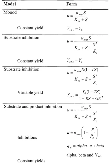
from the theory of enzymatic or chemical reactions. The most frequent relationships
employed suitable for this purpose are summarised by Volesky and Votruba (1992)
as in the following equations. Table 2.1 shows the description of the parameters
used in these equations.
Parameter Description
k Rate of change of the phenomenon
K Active site n Natural number
r Relationship being considered
S Substrate concentration
Table 2.1 Nonlenclature used for the different relationships
kS r =
-3 K+S
kS" r
=
4 K + S"
( -),/K)
1'6
=
k exp .Linear relationship between the rate of the
phenomenon and the reaction Substrate
concentration.
Derived from the Freundlich absorption
isotherm, characteristic for most hydrol)1ic
reactions.
Typical relationships used in fermentation,
represents the rate of change of a phenomenon
controlled by chemisorption of the Substrate
onto one active site such as the molecule of an
enzyme.
Modification of the preceding case where
more than one active site is present on
each bio-catalytic molecule.
Not usual type of rate relationship
recommended for describing the process
dynamics, based on a purely physical
interpretation derived from equations for
movement of a mass point in an
environment characterised by dissipation
forces.
The substance with concentration S is
considered as directly participating in the
dissipation of kinetic energy during the
course of the reaction.
-'-kK r = ---~
7 K+S
kK r
-8 - K
+
sn
Based on the principle of hypothetical
reversible blocking of the active reaction
site by chemisorption of a substance \\-ith
concentration S.
Derived from inhibition of a larger number
of active reaction sites of a certain
biochemical process bottleneck.
Frequently, the use of these rate relationships is made by combination between them
based on superimposition of several phenomena in the given sub-system. Sometimes
this aspect becomes relevant only when it comes to model identification. This is
usually accomplished either by plotting the derived numerical relationships for rates
against concentrations of the substrate or of the product. The plot and correlation of
the rates against each other enables estimation of local yield coefficients or
eventually of their mutual relationships.
The determination of numerical values of the mathematical model parameters IS
based on an appropriate method as an important part of modelling. According to
Volesky and Votruba (1992); these methods can be divided into:
i) linear and non-linear regreSSIOn: based on conventional methods of
mathematical statistics,
ii) momentum analysis of experimental data: using techniques derived from
momentum analysis for expressing numerical values of model parameters
and
iii) adaptive identification and estimation of model parameters: in which the
computer continuously re-evaluates model parameters so that the
behaviour of the process can be predicted and controlled,
In the simulation application, model equations are soh'ed for different initial and
boundary conditions according to a certain scenario based on the planning of
simulation experiments. Simulation studies make possible testing of no\'el or
alternative technological variants of the process such as the change from a batch to
continuous-flow cultivation~ or to the use of an immobilised-cell technology,
The understanding and study of any process, requires a mathematical representation
or model of the process. The process may have an input-output representation or a
time series. The model is based on the prior physical or subjective knowledge about
the process itself, the measured data on the inputs and the outputs, and the physical
and engineering laws governing the working of the process.
If the model is a complete and exact representation of the process, it is called a
deterministic model, and the process is then called a deterministic process. The
parameters of such a model are precisely known, and the model can be used to
produce exact prediction of the process response from the past data. Nevertheless,
most real life processes cannot be represented by this kind of model, because of the
dynamic nature of the process and the lack of information and other uncertainties
being associated with the available data. A model that incorporates noise or
disturbance terms to account for such imprecision in the knowledge of the process is
in that case called a stochastic model.
The design of a control system is usually based upon a linear model of the plant to be
controlled, for the good reason that the assumption of linearity makes the dynamical
behaviour much easier to analyse. In practice, however, all systems are usually
non-linear and, therefore, may exhibit forms of behaviour that are not at all apparent from
the study of the linearised versions. The model is not expected to be a reconstruction
of the process, rather it is intended to serve as a set of operators on the identified set
of inputs. producing sin1ilar output as expected from the process. The problem is
that in real life the process output is usually contaminated \\"ith noise and other
disturbances, \\"hereas ideally the model should follo\\" the true output of the
underlying representatiye process. \\"hich is unknO\\TI. There can be different models
According to previous research about fermentation processes, three different modes
can be distinguished (Ferreira, 1997):
1. Batch fermentation refers to a partially closed system in which most of the
materials required are loaded onto the fermentor, decontaminated before the
process starts and then removed at the end. Conditions are continuously
changing with time, and the fermentor is an unsteady-state system. although
in a well-mixed reactor, conditions can be assumed to be consistent
throughout the reactor at any instant of time.
2. Continuous culture is a technique involving feeding the microorganism used
for the fermentation with fresh nutrients and, at the same time, remoying
spent medium plus cells from the system. A time-independent steady state
can be attained which enables one to determine the relations between
microbial behaviour and the environmental conditions.
3. batch processes are commonly used in industrial fermentation.
Fed-batch fermentation is a production technique in between Fed-batch and continuous
fermentation. They improve control possibilities, such as computer based
fermentation systems. A fed-batch is useful in achieving high concentrations
of product because of high concentrations of cells for a relative large period
of time.
Fermentation processes are used for producing many fine substances such as amino
acids. antibiotics, baker' s yeast enzymes, etc. Among the modes of operation
(batch, fed-batch and continuous). the fed-batch technique is often used in industry
due to its ability to overcome the catabolic repression or glucose effect, \vhich
usually occurs during production of these fine chemicals (Vanichsriratana et aL
1997).
Fed-batch fernlentation can be the best option for some systems in which the
nutrients or any other substrates are only sparingly soluble or are too toxic for adding
process, the limiting substrate is fed without diluting the culture. The culture yolume
can also be maintained practically constant by feeding the gro\\1h limiting substrate
in undiluted form.
Two cases can be considered in fed-batch fermentation: the production of a gro\\ 1h
associated product and the production of a non-growth-associated product. In the
first case, it is desirable to extend the growth phase as much as possible. minimising
the changes in the fermentor as far as specific growth rate, production of interest and
avoiding the production of by-products. For non-growth associated products. the
fed-batch would have two phases: a growth phase, in which the cells are grown to the
required concentration, and then a production phase, in which carbon source and
other requirements for production are fed to the fermentor.
A variable fed-batch is one in which the volume changes with the fermentation time
due to the substrate feed. The way this volume changes is dependent on the
requirements, limitations and objectives of the operator. A proper feed rate. with the
right component constitution, is required during the process. The production of
by-products, which are generally related to the presence of high concentrations of
substrate, can also be avoided by limiting its quantity to the amounts that are required
solely for the production of the biochemical. When high concentrations of substrate
are present. the cells get overloaded, in that, the oxidative capacity of the cells is
exceeded, and due to the Crabtree effect (Reynders et aI, 1997) products other than
the one of interest are produced, reducing the efficacy of the carbon flux. Moreover,
these by-products have shown to even contaminate the product of interest, such as
ethanol production in baker's yeast production, and to impair the cell growth
reducing the fermentation time and its related productivity.
The optimal strategy for the fed-batch fermentation of most organisms is to feed the
growth-limiting substrate at the same rate that the organism utilises the substrate: that
is, to match the feed rate \"ith demand for the substrate. Regardless of the type of
control. both mathematical model a\'ailability and measurement possibilities
intlul'nce the design. The subsequent mathematical model has the follo\\'ing
assuI11ptions: the feed is provided at a constant rate. the production of mass ot'
biomass per mass of substrate is constant during the fermentation time: and a very
concentrated feed is being provided to the fermentor.
Table 2.2 shows the description of the parameters used for the fed-batch fermentation
equations:
Parameter Description
alpha Constant yield
beta Constant yield
F Substrate feed rate
G Constant value defined by experimental data
Kd Specific death rate Ki Inhibition constant
Km Inhibition constant P Product concentration
Pm Maximum product concentration qp Specific production rate of product
R Constant value defined by experimental data
r p Product formation rate
S Substrate concentration in the fermentor
So Substrate concentration in the feed
t Time
T Constant value defined by experimental data u Specific growth rate
Umax Maximum growth rate
V Volume of the fermentor X Biomass concentration
Xo Biomass at the beginning of the fermentation fa Initial value of the yield factor
YyiS Yield factor
Table 2.2 Description of the parameters used in fed-batch fermentation