Inflatable shape changing colonies assembling versatile smart space structures

Author's Accepted Manuscript

Inflatable Shape Changing Colonies

Assem-bling Versatile Smart Space Structures

Thomas Sinn, Daniel Hilbich, Massimiliano

Vasile

PII:

S0094-5765(14)00258-6

DOI:

http://dx.doi.org/10.1016/j.actaastro.2014.07.015

Reference:

AA5139

To appear in:

Acta Astronautica

Received date: 20 December 2013

Revised date: 2 June 2014

Accepted date: 10 July 2014

Cite this article as: Thomas Sinn, Daniel Hilbich, Massimiliano Vasile,

Inflatable Shape Changing Colonies Assembling Versatile Smart Space

Structures,

Acta Astronautica,

http://dx.doi.org/10.1016/j.actaastro.2014.07.015

This is a PDF file of an unedited manuscript that has been accepted for

publication. As a service to our customers we are providing this early version of

the manuscript. The manuscript will undergo copyediting, typesetting, and

review of the resulting galley proof before it is published in its final citable form.

Please note that during the production process errors may be discovered which

could affect the content, and all legal disclaimers that apply to the journal

pertain.

Page 1 of 23 Beijing Conference Paper

Inflatable Shape Changing Colonies Assembling Versatile Smart

Space Structures

Thomas Sinn (corresponding author)

[email protected] t: +44 (0)7411 246 531

Advanced Space Concepts Laboratory

Department of Mechanical & Aerospace Engineering University of Strathclyde

Level 8, James Weir Building 75 Montrose Street

G1 1XJ Glasgow United Kingdom

Daniel Hilbich

[email protected] t: +1 (0) 778 782 4923

Microinstrumentation Laboratory Reconfigurable Computing Laboratory School of Engineering Science Simon Fraser University 8888 University Drive V5A 1S6 Burnaby, BC Canada

Massimiliano Vasile

[email protected]

t: +44 (0)141 548 2326, f: +44 (0)141 552 5105 Advanced Space Concepts Laboratory

Department of Mechanical & Aerospace Engineering University of Strathclyde

Level 8, James Weir Building 75 Montrose Street

G1 1XJ Glasgow United Kingdom

Abstract

Page 2 of 23 antennas that are able to dynamically change their focal point, as well as substructures for solar sails that are capable of steering through solar winds by altering the sails’ subjected area.

Keywords: smart structure, space inflatable, bioinspired, MEMS, nanocomposite polymer

1 Introduction

One of the most expensive features of a modern space mission is the rocket launch [1]. Launch costs can be decreased by reducing the mass and the volume of the spacecraft, which can be achieved either by launching another satellite in the same payload fairing or by delivering the payload using a less powerful, and therefore less expensive, rocket. A viable option to decrease the volume and mass of a space craft is the use of deployables for large structures such as solar arrays, reflectors, concentrators, or even space habitats [2]. A widely used deployable structure today is the umbrella deployable, which is effective but relatively unreliable due to a large number of moving parts [3]. More exotic systems use electrostatic forces to deploy a structure [4] or a spinning assembly to deploy a membrane or web using centrifugal forces [5-6]. A very promising field is the use of inflatable structures due to their simple and reliable deployment mechanism and low storage volume. Inflatable space structures have been around since the 1950s, for example with the ECHO II satellite [7] which deployed an inflatable satellite over 40m in diameter. Since that time, interest in inflatable structures has steadily increased due to their potential to be used in large-volume space habitats, which could play an important role in the manned exploration of our solar system. Aside from using inflatable structures, additional mass and volume can be decreased by enabling a space structure that is able to serve multiple purposes during its mission life. An example of this is a solar energy collector that could serve as a communication antenna by adjusting its shape, and thereby its focal point.

In order to achieve multipurpose structures, extensive research has been undertaken in the field of structures that can change their properties by an external excitement [8]. For example, structural deformation could be induced through an applied electric field, or a change in stiffness could be achieved through an applied temperature change. Unfortunately, most of the adaptive materials available today require a constantly applied actuation force to obtain the desired shape, which results in high power consumption. Other devices are bi-stable, using a short actuation impulse to switch between two different stable states. It is especially important that a space structure can stay in the deformed shape without the necessity of constantly driven actuation due to onboard power constraints. Over the last half century, continuous research and development work has been undertaken in the field of pneumatic devices that mimic biological muscles for actuating mechanical systems, for example in high lift surfaces on planes [9]. Pneumatic muscles were created that shorten when inflated and thereby become capable of lifting substantial loads [10]. Especially interesting for the proposed application are the methods employed by R. Vos [11],[12] and his work on a morphing airfoil that utilizes gas filled elastic pouches that vary their diameter depending on the pressure of the environment. Such an airfoil is able to independently adapt its shape depending on the altitude without the need for further control.

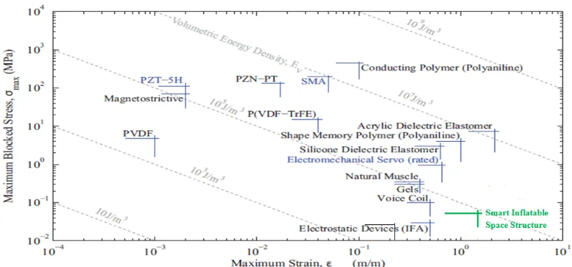
Page 3 of 23 Fig. I: SRI International/DARPA specific energy chart of existing actuators and the developed smart inflatable

space structure (original from Ref. [11]).

The bio inspired concept of a lightweight structure consisting of up to thousands of modular colonies capable of changing their shape is presented in the following sections. The paper outlines the design of the inflatable hyper-elastic cells and their shape changing mechanism, and also includes detailed subsystem descriptions.

2 Design

Page 4 of 23 Fig. II: Schematic of deployment with the release of colonies from

launcher and assembly via free-flying robot.

Another option (shown in Fig. III) would be to eject an assembly robot that has a storage unit filled with stored colonies. After the robot reaches the desired orbit, it will start releasing colonies one after another, letting them inflate and inspecting them for possible damage. The robot can hold on to the assembled structure, inspect the newly deployed colony and add it to the assembled structure.

Fig. III: Schematic of assembling structure via robot with colony storage

Deploying the structure already fully assembled would be also an option. This option is the most desirable as it would make an assembly robot unnecessary; however, the danger of permanent entanglement is substantial, especially when deploying very large structures.

Page 5 of 23 Another application could be as a substructure for a concentrator or reflector of a spacecraft which can be deployed via inflation, taking advantage of the very low stored volume of the structure during launch. The focal point of the concentrator can then be adjusted by changing the curvature of the structure. This capability is required for applications such as space based solar power collectors, which must direct solar radiation to a single point in a geostationary orbit in order to have one stationary receiver on the Earth’s surface. Over the course of a day, the incoming light of the sun needs to be redirected by an adaptive mirror or concentrator on the surface of the solar panel collector.

An application for planetary or terrestrial rovers can be envisioned as well. The smart cellular structure could be actuated to move similar to a snake over any kind of terrain, or even swim through water. Due to the fact that the actuation works with inflating and deflating the cells, the soft robot rover can actually squeeze through small openings giving it an advantage compared to conventional robots. Further applications of this soft robot can be in disaster relief, for example to search for survivors in a collapsed building after an earthquake.

2.1 Modular Colonies

Page 6 of 23 Fig.IV: 3D realization of one cell connected to pressure source (centre) surrounded by inflatable cells connected via

MEMS valves

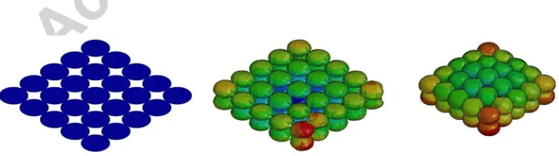
LS-DYNA™ inflation simulations have been carried out to observe the dynamic deployment behaviour of the structure. The initial shape was modelled in the LS-DYNA™ pre-processor LS-PrePost™. LS-DYNA™ is a well known software used in the industry for nonlinear dynamic simulations. Its development for airbag deployment simulations is especially interesting for this application. The control volume method was used to simulate the inflation of the cells. In this approach, a mass flow rate into the enclosed structure needs to be defined. The mass flow required for the control volume method was calculated by employing simple geometries and thermodynamic equations by using the assumption of dealing with an ideal gas. The simulation used a 5x5 cell array with a thickness of two cells. Each cell in the simulation had an initial diameter of 14.5cm (10cm x 10cm square diagonal) and was inflated with an internal differential pressure of 150Pa. The LS-DYNA deployment simulation can be seen in Fig. V. The whole simulation lasted two seconds, with the three frames shown in Fig V being one second apart.

Page 7 of 23

2.2 Control Architecture

In this system design, gas flow and electrical signals are routed throughout the cells in a colony enabling any configuration of inflated cells to be achieved. This section discusses the overall architectural details of a colony and the system as a whole which enables this functionality.

2.2.I Electrical Routing 

The first consideration is given to electrical routing and communication within a colony. Each cell will require a number of electrical signals to control individual components within the cell: one signal per valve, and two signals per pressure sensor. Research in valve architectures described later in the article will show that roughly 2.5 valves and 1 pressure sensor per cell will provide a suitable architecture. This means that there are, on average, 4.5 electrical connections per cell. If all cells in a 5x5 colony are routed to a central controller, this will result in over 100 electrical I/O connections to the controller and over 200 intercellular electrical interconnects. The number of intercellular connections and controller I/Os can be calculated by analysing Fig. VI; from the figure, it can be seen that if there are 24 cells (excluding the central cell) each carrying 4.5 routing signals to a central controller, then by multiplication the total number of I/O connections to the controller is over 100. The total number of intercellular connections (that is, the total number of connections across cell boundaries summed over the entire colony) is slightly less trivial to calculate. In Fig. VI, a single coloured line is used to represent all routing signals from a given cell. The red ‘corner’ cell routing crosses four cell boundaries to arrive at the central cell, the green (cell below) crosses three, and blue crosses two. If the red routing is 4.5 signals and crosses 4 cell boundaries, then that is 18 intercellular connections total. The green and blue signals represent 13.5 and 9 such connections respectively. When all cells are accounted for, the total number of intercellular connections is over 200. The number of controller I/O connection requirements and intercellular interconnects becomes increasingly large as the colony size increases, which is quite prohibitive to the feasible colony size.

Fig. IVI: Electrical routing required for cells within a colony.

The first improvement to the system’s electrical routing is to note that not all signals within a cell will need to operate simultaneously. For example, valve operations within a cell can be performed successively rather than concurrently. Similarly, it will be demonstrated in Section 2.4.2 that the pressure sensor needs only to sense or deliver voltage at one time, but never both. Finally, although valves and pressure sensors will need to function concurrently, for example during inflation when a valve must be open while pressure is continuously sensed to determine the fill level, valve operations will require on the order of 10s to 100s of seconds, while pressure sensor operations are in the order of milliseconds. Thus, it will not impact system performance to intermittently switch from a valve operation to momentarily check on pressure. Thus, the number of active signals per cell is reduced to one assuming the appropriate control signals are added.

controller m switched b other malfu over the re adding sho prudent as greatly inc distributed

Fig. VII: a)

  2.2.II Co The com system. Th through ne inherent tra and the com are require approach w the whole s analysis us routing pro Fig. VIII, a

malfunction, th between the co function, one o emaining slave ort range wirel both the flexi creased. The s electronics on

) Schematic of

onnection Va

mplexity of the he hard design eighbouring cel ade-off in the d mplexity of the ed, with more with a valve on structure comp ing Graph The oblems [17] bu are discussed to

Fig. VIII

he controller a ontrollers. For of the slave co es through eith less communic ibility to comm stratospheric b n a flexible stru

f controllers dis

alves 

e system, and t requirements lls, and that an design process e structure, is a operations req n each cell side paratively heav eory (particular ut is beyond th

o demonstrate

I: Single path v

and software a example, if th ontrollers is the her a wired or cation capabili municate acros alloon iSEDE ucture with wir

stributed over exper

to some extent are that every ny configuratio s; the approach also the approa quiring that the e, meaning eac vy and complex

rly relating to H he scope of this

examples of th

vs. tree path vs

architecture mu he master cont

en notified via r short range w

ities rather tha ss the entire st experiment [ eless communi

surface of colo riment iSEDE

t the weight, is cell is accessi on of cells bein h that uses the

ach that uses th e gas be vente ch cell can exc x. In the future Hamiltonian Pa s paper. Severa hese design con

s. full path (blu

ust be set up troller in Fig. a a communica wireless conne an wired conn tructure and a 16] which suc ication can be

ony b) Distribu [12]

highly depend ible by the cen ng inflated or fewest number he most gas sin ed into the env change gas flow e, this type of aths) which ha al basic connec nsiderations.

ue cell in centre

such that the m VIIa fails due ation timeout ection. At this

ections betwee adaptability to

ccessfully prov seen in Fig. VI

uted electronic

dent on the num ntral pressure s

deflated is ach r of valves, thu nce more comp vironment. On w with all of it problem is sui as previously be

ction valve arc

e: pressure sou

Page 8 master status c e to damage or

and assumes c stage in the d en controllers any malfuncti ved the princi IIb.

of inflatable sa

mber of valves source by som hievable. There us reducing the plex valve oper n the other han ts neighbours, itable for an in een applied to chitectures, sho

urce)

8 of 23 can be r some control design, seems ion are iple of atellite

Page 9 of 23 The three path types considered are the single path with just two valves on each cell for 2D and 3D colonies, the full path with 4 valves in 2D (6 in 3D) and the tree solution in-between with three to four valves.

The amount of actuation and therefore the amount of used gas mass highly depends on the application and planned mission. For example if the mission is quite short, it may be better to use a design that requires fewer valves, since more of the gas would be expendable. On the other hand, a larger mission with many dynamic reconfigurations of the structure would require a large amount of gas; to minimize wasted gas in this case, it would be more feasible to increase the number of valves and complexity in the design. Essentially, each mission must minimize cost as a function of gas mass, valve mass, and complexity.

To achieve a checkerboard pattern, where each cell is in a state alternate to its nearest neighbours, then the number of operations and the path of the gas will be different in each architecture. Table I shows the number of valves required in each architecture, as well as the number of gas units required to achieve this pattern due to inflation and deflation operations. Note that in this analysis, it is assumed that the only outlet valve allowing the gas to escape to environment is at the central cell. To achieve the checkerboard pattern, for example in the single path approach, all the cells have to be inflated fist until the air reaches the last cell. Following this the air from all the cells except of the last one will need to be realised from the centre cell and is therefore lost. To inflate the third last cell in order to create the desired pattern all cells until the third last cell needs to be inflated again and so on. Depending on the cost function (as yet undetermined) which operates based on the cost of gas and the number valves, it can be seen that there will be a large difference between the Single and Full architectures for this application.

Table I: Required gas units and valves for each path design to achieve checkerboard pattern (without outlet valves at each cell)

Single Tree Full

Required Valves 24 24 40

Required Gas units 156 28 24

2.2.III Outlet Valves 

The amount of used gas can be further reduced by adding an outlet valve to each cell to release the gas into outer space. By adding these outlet valves, each cell can deflate by itself and is not required to deflate all the surrounding cells. The same analysis of the checkerboard pattern is presented in Table II, except with outlet valves at each cell.

Table II: Required gas units and valves for each path design to achieve checkerboard pattern (with outlet valves at each cell)

Single Tree Full

Required Valves 48 48 64

Required Gas units 24 20 18

As previously mentioned, the added mass and complexity of the additional valves in contrast with the mass reduction of the required inflation gas must be addressed for each mission separately. From a comparison of Table I and Table II, it can be seen that the extreme case to minimize the number of valves and complexity requires 24 valves and 156 gas units for the single tree without outlet valves. While minimizing gas use requires 64 valves and only 18 gas units for the fully connected tree with outlet valves on each cell. It should also be noted that these calculations assume that all valves and cells remain operational. In the case of the catastrophic failure of a cell or multiple cells, the damaged cells need to be isolated via permanent closure of neighbouring valves. In this case, an architecture with increased valve connectivity has the added benefit of being able to isolate damaged cells and reroute gas flow in the case of failure.

2.3 Inflatable Cell Design

Page 10 of 23 inflated cell to self-deflate when exposed to the vacuum of space. Although the requirements for elasticity and flexibility of the cell membrane are crucial, it is also important that the material selected can be incorporated with all other components into the overall design of the cell. Therefore, the ability of the material to be used in an overall fabrication process which allows for seamless integration all components into a single cell becomes a large design driver for the material. For this reason, a silicone based elastomer material such as polydimethylsiloxane (PDMS) has been selected as the membrane material, which can be spun into thin sheets, cured, and then bonded at the cell borders using well studied PDMS bonding techniques, such as oxygen plasma bonding, corona discharge, or adhesives [18]. This method allows for the integration of other MEMS components into the cell which are fabricated using similar PDMS nanocomposite polymer (NCP) techniques, such as hydrogel-based valves, mechanical interconnects and electrical routing components.

2.4 MEMS Devices

MEMS technology encompasses the design, fabrication, and applications of micro-scale devices or structures that have mechanical, electromechanical, or electromagnetic components. Though a formal definition has proved to be elusive, a MEMS device typically contains structures with <1-100μm feature sizes, and is no more than several millimetres in one dimension as a whole [19]. Examples of MEMS technologies range from simple microstructures such as a silicon micro bridge, to more complex devices such as microfluidic pumps and chemical sensors with fully integrated microelectronics [19]. These devices are typically fabricated using processes derived from industry-standard micro fabrication techniques such as deposition, lithography, and etching, which have been well studied through extensive use in the microelectronics industry. More recently, MEMS technology has incorporated new materials, such as nanoparticle doped polymers, to suit a growing list of applications [20]; these new materials and applications often require the development of novel micro fabrication processes which are unique from those typically found in the microelectronics industry.

Perhaps the most prolific of all MEMS devices are the transducers: devices which convert measurable physical phenomena into electrical signals and vice versa (sensors and actuators, respectively). The last 30 years has seen a vast increase in the number of MEMS sensing devices suiting wide variety of sensing modalities [21], such as various chemical sensors, photometers, temperature sensors, mechanical and inertial force sensors, magnetic field sensors, air and gas flow sensors, etc. Though these MEMS sensors have traditionally been given more focus than their actuator counterparts, more and more actuators are being developed, for example microfluidic pumps and valves, mechanical gears and motors, micro heaters, and electromagnetic field generators.

The benefits of a MEMS device versus its macro scale counterpart are typically reliability, cost, and functionality. Reliability is improved in part due to batch fabrication processes with highly controllable processing parameters resulting in high yield production capabilities. Another important aspect is that MEMS devices are often less susceptible to mechanical failure due little to no mechanical motion within the device, which can be seen for example in MEMS sensors [21]. Cost is also improved from batch fabrication, but is also greatly improved by a reduction in materials and power requirements. Improvements in functionality can generally only be analyzed in specific applications; however, some themes can be generally applied. Less variation at the micro scale often results in more accurate measurements, for example in a temperature sensor where a relatively large active measuring region will return the average of the temperatures within that region, while a smaller measuring region will more accurately show temperature variations invisible to the larger counterpart. Sensitivity is therefore increased at the micro scale, and other benefits can also be exploited, such as increased surface area to volume ratios.

Polymer MEMS devices in particular are increasing in popularity due to several advantages not found in traditional silicon devices, such as flexibility, opacity, biocompatibility, optical properties, and the ability to produce devices using large scale batch fabrication, among others [16]. Examples of these devices which are relevant to the design of inflatable cells are discussed in further detail in the following sections.

2.4.I Microvalves 

In order to achieve a given cell configuration, a central pressure source is required to supply the gas flow, and intercellular valves are required to direct the gas flow through to the desired cells; in this section, the microvalve component of the design is discussed using examples of existing MEMS technology.

Page 11 of 23 weight, reliable valve which is normally closed (blocks fluid or gas flow without consuming power), with minimal restrictions on valve actuation frequency since dynamic reconfigurations are not expected over very short periods of time. For this reason, a mechanically flexible diaphragm-based microvalve which uses a thermally responsive hydrogel actuator and a conductive nanocomposite polymer (C-NCP) heater element [23] has been selected for this design. An illustration of this valve is given in Fig. IX. The C-NCP heaters that provide valve actuation are doped using tungsten nanoparticles, and require a single electrical I/O for the heater element. The valves measure 100-200μm in diameter, and have been measured to deflect (increase in size) 100μm upon heating from room temperature (20°C) to 32°C over a period of 50-300 seconds. Although these valves meet the given design requirements, they have not been tested in space, and would need to be characterized under these conditions, particularly for deflection characteristics at low temperatures. Additionally, since this is a thermally responsive valve design, the effectiveness would be limited to environments with relatively low temperature variations.

Fig. IX: Thermally responsive hydrogel-based microvalve [23] (used with permission)

Commercially available devices were also considered; however, at this time off-the-shelf valves and pumps do not exist which meet the design requirements. In particular, existing pumps are relatively complex and require multiple electrical I/O connections in order to function. This aspect alone is too problematic given the electrical interconnect structure of design, discussed in the Control Architecture section. For the interested reader, some current companies providing commercial microfluidic devices are ThinXXS (microvalves), Debiotech (implantable micropumps), Schwarzer Präzision (micropumps), and Bartels (micropumps).

2.4.II Pressure Sensors 

Page 12 of 23 Fig. X: (a) Pressure sensor placed on outside of cell membrane. (b) With applied pressure, the distance between

metallization layers will vary, altering the capacitance of the sensor.

In this sensor design, a voltage input to the capacitive sensor is routed to an output pin of the microcontroller. The microcontroller should also have an internal hardware resistor of a known value (or, an external resistor can be added), and an input pin for voltage sensing. The resistor and capacitor form an RC circuit with a time constant that varies according to the capacitance of the sensor. In order to determine the internal differential pressure, the controller sends periodic DC voltage outputs to the RC circuit, and measures the voltage across the capacitor through the voltage sensing input pin as the circuit relaxes. By measuring this relaxation voltage over time, the time constant can be calculated within the microcontroller, and thus the capacitance can be determined. This capacitance is then compared to a pre-determined calibration table to find the internal differential pressure.

2.4.III  Electrical Routing and Interconnects 

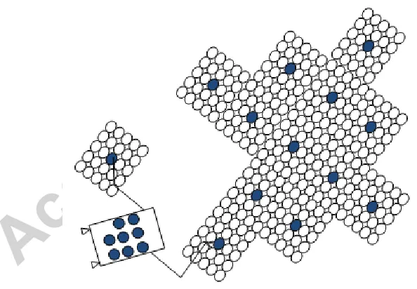
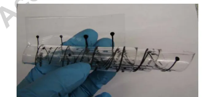
As mentioned previously, electrical routing between neighbouring cells and to a central microcontroller will be required. The routing fabrication and integration is discussed here. The design requirements are once again that this component is lightweight and is easily integrated into the overall fabrication process. Since the previous processing steps include PDMS and NCP components, an electrically conductive multiwalled carbon nanotube (MWCNT) C-NCP routing solution is presented, which will be attached to and run along the cell membrane and is easily integrated into PDMS-based micro fabrication processes [25]. In [25], the fabrication and characterization of a flexible C-NCP routing scheme has been presented, with signal lines which are approximately 500μm by 500μm (with and height respectively) and a resistivity of approximately 10μm. A sample of these flexible routing lines is shown in Fig. XI. The routing signals must travel across cells in order to reach the microcontroller, and are interconnected according to scheme given in [26].

Page 13 of 23

2.4.IV Cell & Colony Mechanical Interconnects 

The final component of the cells is a mechanical interconnect structure which allows neighbouring cells to be fastened together resulting in the modular assembly that have been proposed. Various examples of these mechanical interconnects, which also must allow fluid/gas flow, have been presented by the Microinstrumentation Laboratory at SFU, for example in [27-29]. A scheme with a notched cylinder and hole pair fabricated in silicon allows for both mechanical and fluid interconnects in the same structure [24] and can be integrated in a PDMS-based fabrication scheme. These structures can be seen in Fig. XII and example system level connections can be seen in Fig. XIII.

Fig. XII: SEM image of notched cylinder and hole structures forming both mechanical and microfluidic interconnects [24] (used with permission)

Fig. XIII: Microfluidic board and assembled interconnect components [28] (used with permission)

Page 14 of 23 section; in this scheme, a hydrogel ‘male’ component on one colony is heated (causing it to shrink in volume) and fitted into a ‘female’ component on another colony. When heating ceases, the hydrogel will expand, thus fastening the two colonies together. To detach, the hydrogel is heated once again.

3 Simulation

To observe the behaviour of the developed structure in a space environment, a code has been created to simulate the deployment and shape changing capabilities of the colonies. Such a simulation is necessary due to the fact that the presented structure aims to deploy very large space structures of up to hundreds of meters in diameter. These structures cannot be tested in their full scale on the ground due their low stiffness and the high gravitational forces here on Earth.

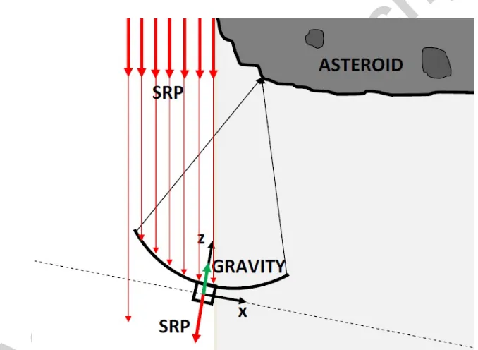
Common very large structures in space include reflectors, parabolic antennas, and concentrators, all of which require a deployment mechanism. Of these applications, a sun concentrator dish was chosen to simulate and validate the capabilities of the smart structure. Such a concentrator can be used to focus solar radiation on an asteroid directly in order to ablate the asteroid and therefore change its trajectory [30]. In this scenario, the dish must be capable of changing its focal point on the surface of the target and must also account for the unusual shape and rotation of an asteroid, thus requiring an adaptive concentrator. Fig XIV shows a sketch of the spacecraft with the curved adaptable concentrator flying into the shadow of the asteroid.

Fig. XIV: Sketch of example application of adaptable sunlight concentrator flying into shadow of asteroid

All the following calculations and simulations are undertaken in the moving reference frame of the spacecraft without any perturbations. The x-axis points towards the velocity direction and the z-axis towards the asteroid. During the mission, the concentrator changes its curvature in the z-direction in order to focus the sun’s energy on the uneven surface of the asteroid. The forces that are applied to the spacecraft are the solar radiation pressure from the sun, having its main component in negative z-direction and the gravity of the asteroid in positive z-direction.

In the following section, the modelling of the single cells, the assembly of the whole structure and the simulation of the adaptable shape concentrator orbiting an asteroid are outlined in detail.

3.1 Discretisation and Modeling

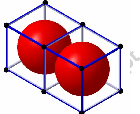
Page 15 of 23 (DOF) nodes. Fig. XV shows the two inflated spherical elements (red) surrounded by two discretisation cubes. Every cell is modelled with 12 beam elements (blue) and 8 nodes (black) on their corners. By assembling a structure consisting of two cells, the beam elements and node elements in the centre are joined resulting in a total of 12 nodes and 20 beam elements for the structure as shown in Fig. XV.

Fig. XV: Two inflatable cells (red) inside discretisation cubes made out of beam elements (blue) in-between nodes (black)

Every array has (ncell x+1) × (ncell y+1)× (ncell z+1) nodes (where ncell i is the number of cells in the i-direction) resulting in a total of 108 nodes for a 5x5x5 cell array. The equation of motion is written with mass matrix M,

damping matrix D and stiffness matrix K. Entries in all three matrices are dynamically modified based on the

inflation and deformation that each cell experiences during the simulation cycle. An example of this change would be the added mass and stiffness while inflating a cell. The coupling terms in the stiffness matrix are especially important for the out of plane deformation of the entire structure.

The equation of motion in Equation 1 is continuously solved in the time domain to obtain the displacement , , and the velocity , , . The input variable is the changing force within the cells and the external forces perturbing the structure. The actuation forces are the internal inflation force Finf and actuation force Fact as well as all

the external forces summarized by Fext. In the developed model, all the forces are applied to the nodes of the cubes

and algorithms have been created to distribute the forces according to their application which is described later in the paper.

inf act ext

+

+

=

+

+

Mq Dq Kq

F

F

F

Page 16 of 23 0,0,0

0 0 0 0 0 0 0 0 0 0

0 12 0 0 0 6 0 12 0 0 0 6

0 0 12 0 6 0 0 0 12 0 6 0

0 0 0 0 0 0 0 0 0 0

0 0 6 0 4 0 0 0 6 0 2 0

0 6 0 0 0 4 0 6 0 0 0 2

0 0 0 0 0 0 0 0 0 0

0 12 0 0 0 6 0 12 0 0 0 6

0 0 12 0 6 0 0 0 12 0 6 0

0 0 0 0 0 0 0 0 0 0

0 0 6 0 2 0 0 0 6 0 4 0

0 6 0 0 0 2 0 6 0 0 0 4

[2]

The element stiffness matrix from Equation 2 is included into the global stiffness matrix by discretisizing each node to obtain the connected beam elements. Equation 3 shows the global stiffness matrix for a six node structure of three nodes in the x-direction and two in the y-direction. The beams with 0 degree orientation are in the x-direction while the beams with 90 degree rotation are perpendicular in the y-direction.

1 11 1 11 1 12 1 12

'

1 12 1 22 2 11 2 12

'

1 12 1 22 2 11 3 11 2 12 3 12

' '

2 12 2 12 2 22 2 22 4 11 4 12

3 1

(0) (90) (0) (90) 0 0 0

(0) (0) (90) 0 (90) 0 0

(90) 0 (90) (0) (90) (0) (90) 0

0 (90) (0) (90) (0) (90) 0 (90)

0 0

K K K K

K K K K

K K K K K K

K

K K K K K K

K − − − − − − − − − − − − − − − − − − − − − + + + + = + + '

2 3 11 3 22 2 12

' '

4 12 3 12 3 22 4 22

(90) 0 (0) (90) (0)

0 0 0 (90) (0) (0) (90)

K K K

K K K K

− − − − − − − ⎡ ⎤ ⎢ ⎥ ⎢ ⎥ ⎢ ⎥ ⎢ ⎥ ⎢ ⎥ ⎢ + ⎥ ⎢ ⎥ + ⎢ ⎥ ⎣ ⎦ [3]

During the inflation and actuation process, the entries of the mass, stiffness and damping matrices change due to the nature of the developed smart structure. The volumetric change of the cell is achieved by adding or removing air or fluid, which also results in a mass change of the model nodes and therefore the entries of the mass matrix.

As the structure is modeled by rotated beam elements, this discretization is only valid for a specific case of the inflated cell. By inflating and deflating these cells, all the entries of the stiffness and therefore the damping matrix change. The changing entries of E, A, I, L, G, and J are obtained either by calculations using simple beam geometries or by experimentation. These calculations and experiments have to be undertaken each time the size, geometry or material of the initial cell changes. The area A and the length L of the structure can be obtained by modeling the cells as beam elements with the same average length and projected area in one direction. As an example, a 14.5 cm inflated spherical cell can be taken resulting in a surface area of 660cm2 _{and a projected surface of 165cm}2 _{in all} three directions . The area A and the length L for each of the four beam elements in one direction are therefore 41.25cm2 _{and 14.5cm respectively. The moment of inertia I and the torsion moment of area J on the other hand are} calculated by using existing equations for simple geometries. For more complex shapes a numerical approach is employed which sums up the infinite mass of all particles multiplied by the square of their distance to the rotational axis. The modulus of elasticity E and the shear modulus G are obtained by a combination of the selected material properties and displacement experiments of bench test cells either in the lab or on CAD and FEM software packages like LS-DYNA.

Page 17 of 23 structure consisting of two inflatable cells (red) with 20 beam elements (blue) and 12 nodes (black). It can be seen that the 4 nodes and the 4 beams in-between the spheres have to account for both cells, therefore the code creates a mean of the entries of these neighboring cells.

The damping matrix in the equation of motion has the main purpose of making the structure controllable. The damping matrix needs to be measured and validated for each application separately; therefore, to keep the simulation simple and scalable, linear damping was assumed.

3.2 Inflation

As an initial condition, all nodes are located in a centre point (e.g. the pressure storage) with an infinitesimal spacing between them. During inflation the differential pressure inside the cells increases which results in an equally applied force on the walls of the cell. Similar to the internal differential pressure of plant’s cell acting on the walls to sustain the integrity of the cell, the inflation force is modelled as an outward force normal to the walls of the cell. The force acting on the wall surface is then split and distributed equally to the four nodes in the corners of the cell wall. If multiple cells are connected together, the forces would cancel each other out if just the sum of forces on every node were taken. For this reason, the code evaluates each nodal cell connection and sums up all the applied forces in a line of connected nodes and applies it to the nodes on the edges of inflating cells. It is also possible to simulate broken cells within the array to observe the deployment behaviour and the obtained shape. The inflation force has a linear slope for a constant time t.

Fig. XVIb shows the qualitative displacement of the nodes of a 5x5x2 cell structure (Fig. XVIa) with an inflation time of 4 seconds and a linear gas inflow. For this simulation, the inflated cell edge length was chosen to be 14.5cm to fit the previously selected dimensions in respect to the 2014 sounding rocket experiment. It can be seen in Fig. XVIb that the whole inflatable structure oscillates slightly after the inflation is complete. Each of the lines in this plot shows the displacement of each node in the structure over time.

Page 18 of 23 Fig. XVI: a) Inflated 5x5x2 cell array, b) Displacement of x-, y-, and z-positions

After inflation is complete, the differential pressure stays constant but it is also possible to apply a leakage to certain cells or the entire array of cells. In practice, this leakage could be caused by micrometeoroid impacts, fabrication errors, degradation of materials, or natural leakage of an inflatable in the space environment.

3.3 Actuation

Page 19 of 23 XVIa is displayed. Fig. XVIIa shows the array before actuation, while Fig. XVIIb shows the array after being actuated once, and Fig. XVIIc shows the increased curvature of the structure after being actuated twice.

Fig. XVIIV: Bottom layer plot of a) inflated structure, b) structure actuated once and c) structure actuated twice

The position over time of all the nodes can be seen in Fig. XVIII. In the first four seconds of the simulation the structure was inflated homogenously. After the oscillation was mostly settled, the first actuation was started at six seconds with a linear increase for four seconds. The second actuation, also shown in Fig. XVIII, was started at 12 seconds and also lasted for four seconds with a linear increase.

Page 20 of 23 Fig. XVIII: Displacement of nodes during inflation in all directions (t<4s) and actuation (t>4s)

3.4 External Forces

Depending on the environment the structure is operated in, the external forces may vary. The main two environments described here are the space and terrestrial environments. Depending on the nature of the application, some forces may only be applied to mass nodes, other forces may act on the inside walls, and others are just applied to one surface on the outside of the structure.

In space, the main external force applied to the structure is gravity, which may include a gravity gradient for very large structures. Even small gravity gradients can affect the structure due its low differential pressure and lightweight nature. The gravitational force is applied to each node towards the centre of gravity with a value changing depending on the distance between the cells. The gravitational force at each node changes at each time step due to the shifting mass during actuation; this is done through the adaptive mass matrix described earlier. Other perturbing forces are solar radiation pressure (SRP) and atmospheric drag which apply a force on the surface of the structure. In order to model these forces in the code, only the nodes on one surface experience the force. These forces depend on the orientation and the shape of the structure. Other forces that can be applied to the model are short term impact forces, for example meteoroids or space debris.

On Earth or planetary bodies, the main force acting on the structure is gravity pulling the structure towards the ground. Obstacles like rocks in the rover’s path or the environment change from e.g. air into water are also being considered. Furthermore, impact and vibration forces become much more dominant for these applications. Compared to space, the external forces on Earth are changing faster, for example the drag force caused by wind gusts which can change directions rather quickly.

Page 21 of 23 force due to solar radiation pressure. While the structure orbits the asteroid, it moves into the shadow of the asteroid making gravity the only external force pulling on the structure. For the simulation, the moving coordinate system of the structure without any perturbation is used.

Fig. XIX: z-axis displacement of structure while flying through the shadow of the asteroid (example)

Fig. XIX shows the z-axis displacement of all the nodes of the structure over time. From the beginning of the simulation, the solar radiation pressure and gravity are acting on the model, even though the solar radiation pressure only reaches its maximum force once the structure is inflated and has its maximum surface area. At 20 seconds, the structure moves into the shadow of the asteroid, subjecting the structure only to the gravity of the asteroid. The structure stays in the shadow until the end of the simulation. From Fig. XIX it can be seen how the model successfully alters the position of the structure due to the applied forces. At 40 seconds, the gravitational pull of the asteroid is strong enough to overcome the momentum accumulated during the first twenty seconds of solar radiation pressure. In the last 40 seconds, the gravity of the asteroid pulls the structure towards its surface resulting in a parabolic shape of the displacement curve.

4 Final Remarks

Page 22 of 23

5 Acknowledgements

The authors wish to acknowledge members of the Microinstrumentation Laboratory and Reconfigurable Computing Laboratory at Simon Fraser University, Canada, for their contributions of images and design ideas. We also like to thank all the Strathclyde students that were involved in the REXUS experiment StrathSat-R and BEXUS experiment iSEDE for their continuous work on building experiments to prove the presented shape changing principle on a sounding rocket and stratospheric balloon.

6 References

[1] J.R. Wertz, D.F. Everett, and J.J. Puschell, eds. Space Mission Engineering: The New SMAD. Hawthorn, CA: Microcosm Press, 2011.

[2] C. Mangenot, J. Santiago-Prowald, K. van't klooster, , N. Fonseca, L. Scolamiero, F. Coromina, P. Angeletti, M. Politano, C. Elia, D. Schmitt, M. Wittig, F. Heliere, M. Arcioni, M. Petrozzi, M. Such Taboada "ESA Document: Large Reflector Antenna Working Group - Final Report," Technical Note TEC-EEA/2010.595/CM. Vol. 1, 2010. [3] C. Mangenot, J. Santiago-Prowald, K. van ‘t klooster, N. Fonseca, L. Scolamiero, F. Coromina, P. Angeletti, M. Politano, C. Elia, D. Schmitt, M. Wittig, F. Heliere, M. Arcioni, M. Petrozzi, M. Such Taboada “Large Reflector Antenna Working Group – Final Report” TEC-EEA/2010.595/CM, ESA, 2010

[4] L. Stiles, H. Schnaub “Electron Flux Deflection Experiments with Coulomb Gossamer Structures” AIAA-2012-1583, 13th AIAA Gossamer Systems Forum as part of 53rd Structures, Structural Dynamics, and Materials and Co-located Conferences, Honolulu, Hawaii, 23 - 26 April, 2012

[5] M.Gärdsback, G. Tibert, D.Izzo: Design considerations and deployment simulations of spinning space webs. 48th AIAA/ASME/ASCE/AHS/ASC Structures, Structural Dynamics, and Materials Conference, Honolulu, HW, 23–26 April, 2007, AIAA-2007-1829.

[6] T. Sinn, M. McRobb, A. Wujek, J. Skogby, f. Rogberg, J. Wang, M. Vasile, G. Tibert “Results of REXUS12’s Suaineadh Experiment: Deployment of a Web in Microgravity Conditions using Centrifugal Forces, IAC-12-A2.3.15, 63rd International Astronautical Congress, Naples, Italy, 1-5 October 2012.

[7] R.E. Freeland, G.D. Bilyeu, G.R. Veal and M.M. Mikulas, "Inflatable Deployable Space Structures Technology Summary" IAF-98-I.5.01, 49th International Astronautical Congress, Melbourne, Australia, 28 September – 2 October, 1998.

[8] I. Chopra, "Review of state of art of smart structures and integrated systems." AIAA journal 40.11 (2002): 2145-2187.

[9] B.Woods, E. Bubert, C.S. Kothera, N.Wereley “Design and testing of a biologically inspired pneumatic trailing edge flap system”, AIAA-2008-2046, AIAA Structures, Structural Dynamics, and Materials Conference,

Schaumberg, IL, April, 2008

[10] N. Tsagarakis, D. G. Caldwell. "Improved modelling and assessment of pneumatic muscle actuators." In Robotics and Automation, 2000. Proceedings. ICRA'00. IEEE International Conference on, vol. 4, pp. 3641-3646. IEEE, 2000.

[11] R. Vos, R. Barrett. "Pressure adaptive honeycomb: a new adaptive structure for aerospace applications." In SPIE Smart Structures and Materials+ Nondestructive Evaluation and Health Monitoring, pp. 76472B-76472B.

International Society for Optics and Photonics, 2010.

[12] R. Vos, R. Barrett. "Method and apparatus for pressure adaptive morphing structure." U.S. Patent 8,366,057, issued February 5, 2013.

[13] T. Sinn, M. Vasile, G. Tibert “Design and Development of Deployable Self-inflating Adaptive Membrane” AIAA-2012-1517, 13th AIAA Gossamer Systems Forum as part of 53rd Structures, Structural Dynamics, and Materials and Co-located Conferences, Honolulu, Hawaii, 23 - 26 April, 2012.

[14] E. B. Wilson, "The Heliotropism of Hydra", The American Naturalist , Vol. 25, No. 293 (May, 1891), pp. 413-433.

[15] T. Sinn, M. Vasile “Bio-inspired Programmable Matter for Space Applications” IAC-12-C2.5.1, 63rd International Astronautical Congress, Naples, Italy, 1-5 October, 2012.

[16]T. Sinn, T. Queiroz, F. Brownlie, L. Leite, A. Allan, A.Rowan, and J. Gillespie ”iSEDE Demonstrator on High Altitude Balloon BEXUS: Inflatable Satellite Encompassing Disaggregated Electronics”, IAC-13-E2.3, 64th International Astronautical Congress (IAC) 2013, 23 – 27 October 2013, Beijing, China

Page 23 of 23 [18] M. A. Eddings, M. A. Johnson, B. K. Gale “Determining the optimal PDMS–PDMS bonding technique for microfluidic devices” Journal of Micromechanics and Microengineering, vol. 18, no. 6, 2008.

[19] C. Richards Grayson, R. S. Shawgo, A. M. Johnson, N. T. Flynn, Y. Li, M. J. Cima, R. Langer “A BioMEMS review: MEMS technology for physiologically integrated devices” Proceedings of The IEEE - PIEEE , vol. 92, no. 1, pp. 6-21, 2004.

[20] C. Liu “Recent Developments in Polymer MEMS” Advanced Materials Volume 19, Issue 22, pages 3783–3790, November, 2007.

[21] R. Bogue “MEMS Sensors: past present future” Sensor Review, Vol. 27, No. 1. 2007, pp. 7-13. [22] K. W. Oh, C. H. Ahn “A review of Microvalves” J. Micromech. Microeng. Vol. 16, No. 5, 2006.

[23] A. Li, A. Khosla, C. Drewbrook, B. L. Gray “Fabrication and testing of thermally responsive hydrogel-based actuators using polymer heater elements for flexible microvalves” Proc. SPIE 7929, Microfluidics, BioMEMS, and Medical Microsystems IX, 79290G (February 14, 2011).

[24] W. P. Eaton, J. H. Smith “Micromachined pressure sensors: review and recent developments” Proc. SPIE 3046, Smart Structures and Materials 1997: Smart Electronics and MEMS, 30 (June 19, 1997).

[25] A. Khosla, D. Hilbich, C. Drewbrook, D. Chung, B. L. Gray “Large scale micropatterning of multi-walled carbon nanotube/polydimethylsiloxane nanocomposite polymer on highly flexible 12×24 inch substrates” Proc. SPIE 7926, Micromachining and Microfabrication Process Technology XVI, 79260L (February 15, 2011).

[26] T. Ueda, S. Jaffer, S. Westwood, B.L. Gray, "Design of Electrical Interconnect for SU-8 Microfluidic Systems" Canadian Conference on Electrical and Computer Engineering, April 2007, pp.5-7.

[27] S. Westwood, S. Jaffer, B.L. Gray, "Enclosed SU-8 and PDMS microchannels with integrated interconnects for chip-to-chip and world-to-chip connections" Journal of Micromechanics and Microengineering, June 2008.

[28] B.L. Gray, S.D. Collins, R.L. Smith, "Interlocking mechanical and fluidic interconnections for microfluidic circuit boards" Sensors and Actuators A, V12, April 2004, pp. 18-24.

[29] S. Jaffer and B.L. Gray, "Mechanically assembled polymer interconnects with dead volume analysis for microfluidic systems" SPIE Photonics West, vol. 6465, January 2007. 

[30] A. Gibbings, M. Vasile, I. Watson, J.M. Hopkins, and D. Burns, "Experimental analysis of laser ablated plumes for asteroid deflection and exploitation." Acta Astronautica (2012).

Highlights

• Smart space structure consisting of colonies of shape changing inflatable cells.  • Developed structure inspired by functionality of motor cells of heliotropism plants.  • MEMS technology enables miniaturization of pumps/valves and electronic architecture.  • Optimal pump, valve and routing architecture depends on application and mission.   • Created mulitbody dynamic code shows shape changing capabilities of structure.